A two-stage blending approach for merging multiple satellite precipitation estimates and rain gauge observations: an experiment in the ...
←
→
Page content transcription
If your browser does not render page correctly, please read the page content below
Hydrol. Earth Syst. Sci., 25, 359–374, 2021
https://doi.org/10.5194/hess-25-359-2021
© Author(s) 2021. This work is distributed under
the Creative Commons Attribution 4.0 License.

A two-stage blending approach for merging multiple satellite
precipitation estimates and rain gauge observations:
an experiment in the northeastern Tibetan Plateau
Yingzhao Ma1 , Xun Sun2,3 , Haonan Chen1,4 , Yang Hong5 , and Yinsheng Zhang6,7
1 Colorado State University, Fort Collins, CO 80523, USA
2 Key Laboratory of Geographic Information Science (Ministry of Education),
East China Normal University, Shanghai, 200241, China
3 Columbia Water Center, Earth Institute, Columbia University, New York, NY 10027, USA
4 NOAA/Physical Sciences Laboratory, Boulder, CO 80305, USA
5 School of Civil Engineering and Environmental Science, University of Oklahoma, Norman, OK 73019, USA
6 Key Laboratory of Tibetan Environment Changes and Land Surface Processes, Institute of Tibetan Plateau Research,

Chinese Academy of Sciences, Beijing, 100101, China
7 CAS Center for Excellence in Tibetan Plateau Earth Sciences, Beijing, 100101, China

Correspondence: Xun Sun (xs2226@columbia.edu)

Received: 27 January 2020 – Discussion started: 17 February 2020
Revised: 3 December 2020 – Accepted: 11 December 2020 – Published: 21 January 2021

Abstract. Substantial biases exist in satellite precipitation es-   son of 2010–2014 in the northeastern Tibetan Plateau. Re-
timates (SPEs) over complex terrain regions, and it has al-         sults show that the blended SPE is greatly improved com-
ways been a challenge to quantify and correct such biases.          pared to the original SPEs, even in heavy rainfall events. This
The combination of multiple SPEs and rain gauge obser-              study can be expanded as a data fusion framework in the de-
vations would be beneficial to improve the gridded precip-          velopment of high-quality precipitation products in any re-
itation estimates. In this study, a two-stage blending (TSB)        gion of interest.
approach is proposed, which firstly reduces the systematic
errors of the original SPEs based on a Bayesian correc-
tion model and then merges the bias-corrected SPEs with
                                                                    1   Introduction
a Bayesian weighting model. In the first stage, the gauge-
based observations are assumed to be a generalized regres-          High-quality precipitation data are fundamental to the un-
sion function of the SPEs and terrain feature. In the sec-          derstanding of regional and global hydrological processes.
ond stage, the relative weights of the bias-corrected SPEs          However, it is still difficult to acquire accurate precipita-
are calculated based on the associated performances with            tion information in the mountainous regions, e.g., the Tibetan
ground references. The proposed TSB method has the abil-            Plateau (TP), due to limited ground sensors (Ma et al., 2015).
ity to extract benefits from the bias-corrected SPEs in terms       Satellite sensors can provide precipitation estimates at a large
of higher performance and mitigate negative impacts from            scale (Hou et al., 2014), but performances of available satel-
the ones with lower quality. In addition, Bayesian analysis         lite products vary among different retrieval methods and cli-
is applied in the two phases by specifying the prior distribu-      mate areas (Yong et al., 2015; Prat and Nelson, 2015; Ma et
tions on model parameters, which enables the posterior en-          al., 2016). Thus, it is suggested to incorporate precipitation
sembles associated with their predictive uncertainties to be        estimates from multiple sources into a fusion procedure with
produced. The performance of the proposed TSB method is             full consideration of the strength of individual members and
evaluated with independent validation data in the warm sea-         associated uncertainty.

Published by Copernicus Publications on behalf of the European Geosciences Union.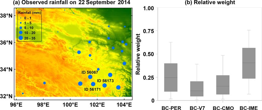
360                    Y. Ma et al.: A two-stage blending approach for merging multiple satellite precipitation estimates

   Precipitation data fusion was initially reported by merg-         The remainder of this paper is organized below: Sect. 2 de-
ing radar–gauge rainfall in the mid-1980s (Krajewski, 1987).      scribes the experiment including the study region and precip-
The Global Precipitation Climatology Project (GPCP) was           itation data. Section 3 details the methodology, including the
an earlier attempt for satellite–gauge data fusion, which         TSB approach, and two existing fusion methods (i.e., BMA
adopted a mean bias correction method and an inverse-error-       and OOR). Results and discussions are presented in Sects. 4
variance weighting approach to develop a monthly, 0.25◦           and 5, respectively. The primary findings are summarized in
global precipitation dataset (Huffman et al., 1997). Another      Sect. 6.
popular dataset, the Climate Prediction Center Merged Anal-
ysis of Precipitation (CMAP), included global monthly pre-
cipitation with a 2.5◦ × 2.5◦ spatial resolution for a 17-year    2   Study area and data
period by merging gauges, satellites, and reanalysis data us-
                                                                  The study domain is located in the upper Yellow River basin
ing the maximum likelihood estimation method (Xie and
                                                                  of the NETP (Fig. 1). As shown in the 90 m digital eleva-
Arkin, 1997). Since then, several blending approaches have
                                                                  tion data, the altitude ranges from 785 m in the northeast
been developed to generate gridded rainfall products with
                                                                  to 6252 m in the southeast. The total annual precipitation is
higher quality by merging gauge, radar, and satellite obser-
                                                                  around 500 mm, and the annual mean temperature is 0.7 ◦ C
vations (e.g., Li et al., 2015; Beck et al., 2017; Xie and
                                                                  (Cuo et al., 2013). To avoid snowfall contamination in the
Xiong, 2011; Yang et al., 2017; Baez-Villanueva et al., 2020).
                                                                  gauge observation in the cold season, satellite and ground
Overall, these fusion methods follow a general concept by
                                                                  precipitation data from the warm season (May to September)
eliminating biases in satellite and radar-based data and then
                                                                  of 2010 to 2014 are collected for the case study.
merging the bias-corrected satellite and radar estimates with
                                                                     Four mainstream SPEs are used, including Precip-
point-wise gauge observations. However, these efforts might
                                                                  itation Estimation from Remotely Sensed Informa-
be insufficient for quantifying the predicted data uncertainty.
                                                                  tion using Artificial Neural Networks – Climate Data
Some blended estimates are also partially polluted by the
                                                                  Record (PERSIANN-CDR) (Ashouri et al., 2015), Trop-
poorly performing individuals (Tang et al., 2018).
                                                                  ical Rainfall Measuring Mission (TRMM) Multi-satellite
   This paper develops a new data fusion method that en-
                                                                  Precipitation Analysis (TMPA) 3B42 version 7 (3B42V7)
hances the quantitative modeling of individual error struc-
                                                                  (Huffman et al., 2007), National Oceanic and Atmospheric
tures, prevents potential negative impacts from lower quality
                                                                  Administration (NOAA) Climate Prediction Center (CPC)
members, and enables an explicit description of a model’s
                                                                  Morphing Technique Global Precipitation Analyses Ver-
predictive uncertainty. In addition, a Bayesian concept for ac-
                                                                  sion 1 (CMORPH) (Xie et al., 2017), and the Integrated
curate rainfall estimation is proposed based on these assump-
                                                                  Multi-satellitE Retrievals for the Global Precipitation
tions. The Bayesian analysis has the advantage of a statistical
                                                                  Measurement (GPM) mission V06 Level 3 final run prod-
post-processing idea that could yield a predictive distribution
                                                                  uct (IMERG) (Huffman et al., 2018). Basic information
with quantitative uncertainty (Renard, 2011; Shrestha et al.,
                                                                  on the SPEs is shown in Table 1. The IMERG has a
2015). For example, a Bayesian kriging approach, which as-
                                                                  0.10◦ × 0.10◦ resolution, and other SPEs have a spatial
sumes a Gaussian process of precipitation at any location and
                                                                  resolution of 0.25◦ × 0.25◦ . To eliminate the scale difference
considers the elevation a covariate, is developed for merg-
                                                                  in the fusion process, IMERG is resampled from 0.10 to
ing monthly satellite and gauge precipitation data (Verdin
                                                                  0.25◦ using the nearest neighbor interpolation method in
et al., 2015). A dynamic Bayesian model averaging (BMA)
                                                                  advance.
method, which shows better skill scores than the existing
                                                                     The China Gauge-based Daily Precipitation Analy-
one-outlier-removed (OOR) method, is applied for satellite
                                                                  sis (CGDPA) is used as ground precipitation source. It is de-
precipitation data fusion across the TP (Ma et al., 2018; Shen
                                                                  veloped based on a rain gauge network of 2400 gauge sta-
et al., 2014). Given the challenges of quantifying precipi-
                                                                  tions in mainland China using a climatology-based optimal
tation biases in regions with complex terrain (Derin et al.,
                                                                  interpolation and topographic correction algorithm (Shen
2019), continuous efforts are required to extract the potential
                                                                  and Xiong, 2016). The 34 grid cells with the gauge sites
merit of Bayesian analysis for this critical issue.
                                                                  in the regions of interest are assumed as ground refer-
   In this study, a two-stage blending (TSB) approach is
                                                                  ences (GRs), and all of the grid cells are independent from
proposed for merging multiple satellite precipitation esti-
                                                                  the Global Precipitation Climatology Center (GPCC) sta-
mates (SPEs) and ground observations. The experiment is
                                                                  tions, which are used for bias correction of the TRMM/GPM-
performed in the warm season (from May to September) dur-
                                                                  era data (e.g., 3B42V7 and IMERG) and CMORPH (Huff-
ing 2010–2014 in the northeastern TP (NETP), where a rela-
                                                                  man et al., 2007; Hou et al., 2014; Xie et al., 2017; Joyce et
tively denser network of rain gauges is available compared to
                                                                  al., 2004).
other regions of the TP. The TSB method is expected to help
with the exploration of multi-source/scale precipitation data
fusion in regions with complex terrain.

Hydrol. Earth Syst. Sci., 25, 359–374, 2021                                         https://doi.org/10.5194/hess-25-359-2021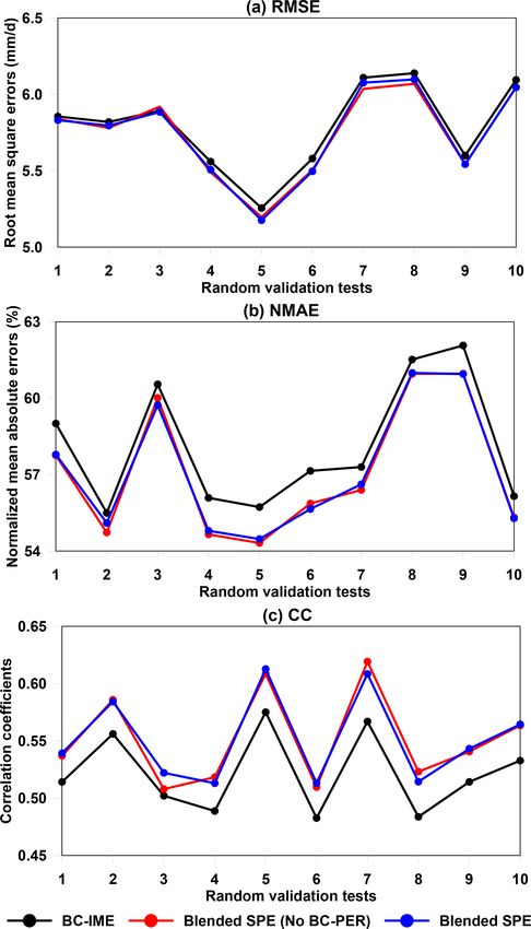
Y. Ma et al.: A two-stage blending approach for merging multiple satellite precipitation estimates                                   361

Figure 1. Spatial map of the topography and GR network used in the study, where 27 black cells are used for model calibration and 7 red
cells are for model verification.

Table 1. Basic information of the original SPEs used in this study.

         Short          Full name               Temporal         Spatial     Input        Retrieval              References
         name           and details             resolution     resolution    data         algorithm
         PERCDR         Precipitation             Daily      0.25◦ × 0.25◦   Warm         Adaptive artificial    Ashouri et al.
                        Estimation from                                      season       neural network         (2015)
                        Remotely Sensed                                      from 2010
                        Information using                                    to 2014
                        Artificial Neural
                        Networks
                        (PERSIANN)
                        Climate Data
                        Record (CDR)
         3B42V7         TRMM Multi-               Daily      0.25◦ × 0.25◦   Warm         GPCC monthly           Huffman et al.
                        satellite                                            season       gauge observation      (2007)
                        Precipitation                                        from 2010    to correct this bias
                        Analysis (TMPA)                                      to 2014      of 3B42RT
                        3B42 Version 7
         CMORPH         NOAA Climate              Daily      0.25◦ × 0.25◦   Warm         Morphing               Xie et al. (2017)
                        Prediction Center                                    season       technique
                        (CPC) Morphing                                       from 2010
                        Technique                                            to 2014
                        (CMORPH) Global
                        Precipitation
                        Estimates Version 1
         IMERG          Integrated Multi-         Daily      0.10◦ × 0.10◦   Warm         2017 version of        Huffman et al.
                        satellitE Retrievals                                 season       the Goddard            (2018)
                        for the Global                                       from 2010    profiling
                        Precipitation                                        to 2014      algorithm
                        Measurement
                        (GPM) mission V06
                        Level 3 final run
                        product

https://doi.org/10.5194/hess-25-359-2021                                                 Hydrol. Earth Syst. Sci., 25, 359–374, 2021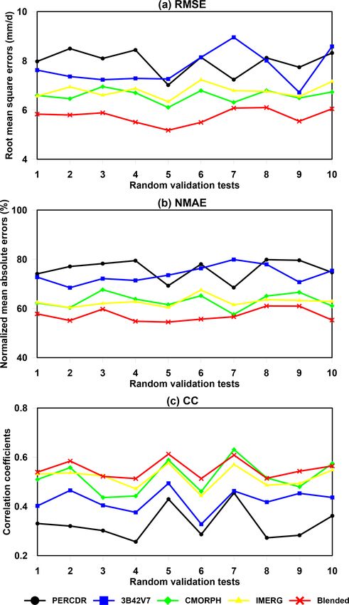
362                         Y. Ma et al.: A two-stage blending approach for merging multiple satellite precipitation estimates

Figure 2. The diagram of the proposed TSB algorithm.

3     Methodology                                                             lognormal, Gaussian, and gamma distribution for the GRs is
                                                                              examined graphically by using a probability–probability (PP)
3.1     TSB                                                                   plot at the training sets (Fig. 3). It is found that the usage of
                                                                              a gamma distribution is more reliable as the associated PP
The diagram of the TSB method is shown in Fig. 2. Stage 1                     plot is closer to the diagonal line than the others. For each
is designed to reduce the bias of the original SPEs based on                  satellite product, the gamma distribution is parameterized as
the GRs at the training sites with a Bayesian correction (BC)                 follows:
procedure. In Stage 2, a Bayesian weighting (BW) model is
used to merge the bias-corrected SPEs.

                                                                                            αi
                                                                              R ∼ 0 αi ,         ,                                          (1)
                                                                                            µi
3.1.1    Bias correction

(a) Model structure                                                           where i is the number of satellite products, and αi , µi , and
                                                                               αi
                                                                              µi are the shape, mean, and rate parameters of the gamma
Let R(st) denote near-surface precipitation at the GR cell s                  distribution, respectively. Let the ith SPE Yi and the associ-
and the tth day. The original SPEs and bias-corrected SPEs of                 ated terrain feature Z be covariates related to the GRs; the
PERCDR, 3B42V7, CMORPH, and IMERG at the GR cell s                            mean µi in Eq. (1) can be described with generalized linear
and the tth day are defined as (Y1 (s, t), Y2 (s, t), . . . , Yp (s, t)       regression of covariates Yi and Z, which is written as fol-
and (Y10 (s, t), Y20 (s, t), . . . , Yp0 (s, t)), respectively. For simpli-   lows:
fication purposes, and without losing generality, these data at
a particular GR cell and day will be denoted by R, (Y1 –Y4 ),                 log (µi ) = δi + βi · log (Yi ) + γi · Z,                            (2)
and (Y10 –Y40 ), while for all GR cells and days, they will be
denoted in bold R, (Y1 –Y4 ), and (Y01 –Y04 ).                                where Z, ranging from 0 to 1, is the normalized elevation fea-
   In Stage 1, we perform a conditional modeling of GRs on                    ture of each site. θi = {αi , δi , βi , γi } (i = 1, . . . , 4) is summa-
each SPE, i.e., the probabilistic distribution f (R) to improve               rized as a parameter set and will be estimated in the Bayesian
the accuracy of the original SPEs. Given that an appropriate                  framework. In the following, Z will be denoted as the collec-
assumption of f (R) is necessary, the goodness-of-fit of the                  tion of the normalized elevation feature for all training data.

Hydrol. Earth Syst. Sci., 25, 359–374, 2021                                                        https://doi.org/10.5194/hess-25-359-2021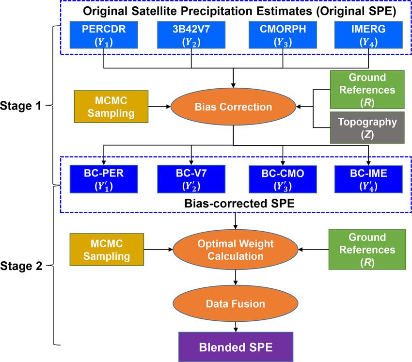
Y. Ma et al.: A two-stage blending approach for merging multiple satellite precipitation estimates                                                            363

Figure 3. (a) The histogram density plot and (b) the corresponding probability–probability plot of GRs at the training grids in the warm
season of 2014 in the NETP, where the red, blue, and green lines shows the fitted gamma, lognormal, and Gaussian distribution, respectively.

  According to Bayes’ theorem, the posterior probability                model, the MCMC converges very quickly. Thus, we run a
density function (PDF) of parameter set θi is expressed as              chain of length 2000, removing the first 1000 iterations as
                                                                        the warm-up period and retaining the second 1000 iterations.
f (θi |R, Yi , Z) ∝ f (R|θi , Yi , Z) f (θi ) ,                 (3)     The parameter samples of these 1000 iterations are the sam-
                                                                        ples of the posterior distribution f (θi |R, Yi , Z).
where f (θi ) is the prior distribution and implies parameter
information other than GR and SPE data, and f (R|θi , Yi , Z)           (c) Bayesian inference
is the likelihood function that defines the conditional proba-
bility of GRs on the SPE and elevation. The priors of f (θi )           Based on the posterior distribution of parameter set θi of each
are initialized as a Cauchy distribution, with αi in terms of           SPE, calculating the bias-corrected SPE R ∗ at new site is of
its location at zero and scale as σαi in Eq. (4), and Gaussian          interest. It can be quantitatively simulated from its posterior
distribution, with δi βi γi in terms of its mean at zero and stan-      distribution in Eq. (8) using the associated SPE Yi∗ , normal-
dard deviation (SD) at σδi σβi σγi in Eqs. (5)–(7), respectively.       ized elevation Zi∗ , and training data R, Yi Z:
                                                                                                                  Z
αi ∼ Cauchy 0, σαi                                             (4)            ∗
                                                                                  |Yi∗ , Zi∗ , R, Yi , Z                f R ∗ , θi |Yi∗ , Zi∗ , R, Yi , Z dθi . (8)

                                                                       f R                                    =
δi ∼ Normal 0, σδi                                             (5)

βi ∼ Normal 0, σβi                                             (6)      Following the rule of joint probabilistic distributions, the
γi ∼ Normal 0, σγi

                                                               (7)      right term inside the integral of Eq. (8) can be written as
                                                                        f R ∗ , θi |Yi∗ , Zi∗ , R, Yi , Z =f R ∗ |Yi∗ , Zi∗ , R, Yi , Z, θi

Given that the assumption of the weakly informative priors
                                                                                                           f θi |Yi∗ , Zi∗ , R, Yi Z .

ensures the Bayesian inference in an appropriate range (Ma                                                                                    (9)
et al., 2020b), the hyperpriors of σαi , σδi σβi , and σγi are spec-
                                                                        Given that the new bias-corrected SPE R ∗ is independent
ified as 2, 10, 10, and 10, respectively.
                                                                        from the training data, the first term of the right side in Eq. (9)
(b) Parameter estimation                                                is transformed as
                                                                        f R ∗ |Yi∗ , Zi∗ , R, Yi , Z, θi = f R ∗ |Yi∗ , Zi∗ , θi .

                                                                                                                                      (10)
The estimation of the posterior distribution f (θi |R, Yi , Z)
in Eq. (3) becomes difficult as its dimension grows with the            Since the parameters θi are only dependent upon the training
number of parameters (Renard, 2011; Ma and Chandrasekar,                data RYi , Z, the second term of the right side in Eq. (9) is
2020). Robertson et al. (2013) obtained the maximum a pos-              expressed as
teriori (MAP) solution for model parameters using a stepwise
                                                                        f θi |Yi∗ , Zi∗ , R, Yi , Z = f (θi |R, Yi , Z) .

method. Here, the Markov chain Monte Carlo (MCMC) tech-                                                                         (11)
nique with its sampling algorithm as the No-U-Turn Sam-                 Therefore, the predictive PDF of R ∗ in Eq. (8) is written be-
pler (NUTS) variant of Hamiltonian Monte Carlo in the Stan              low:
program is performed to address this issue (Gelman et al.,                                         Z
2013). The sampling records of model parameters are ob-                 f R |Yi , Zi , R, Yi , Z = f R ∗ |Yi∗ , Zi∗ , θi
                                                                             ∗ ∗     ∗

tained based on the training data in the warm season of 2014
in the NETP. Since we only have four parameters in this                                                                f (θi |R, Yi , Z) dθi .               (12)

https://doi.org/10.5194/hess-25-359-2021                                                       Hydrol. Earth Syst. Sci., 25, 359–374, 2021
364                         Y. Ma et al.: A two-stage blending approach for merging multiple satellite precipitation estimates

Since there is no general way to calculate the associated inte-       3.2     Comparison model
gral in Eq. (12), the prediction is performed using the MCMC
iterated samplings (Renard, 2011). As for each SPE, a nu-             3.2.1    BMA
merical algorithm is suggested below, where nsim stands for
the replicate of the post-convergence MCMC samples and is             The BMA method is a statistical algorithm that merges pre-
set as 1000 in the case study. Thus, the predicted samples            dictive ensembles based on the individual SPE at the training
for R ∗ in Eq. (12) are iterated (k = 1 : nsim ) as follows:          period in regions of interest. Here, the BMA result refers to
                                                                      the ensemble SPE. Based on the law of total probability, the
  1. For the ith satellite product, randomly select a param-          conditional probability of the BMA data on the individual
     eter sample θi = {αi , δi , βi , γi } from the MCMC sam-         SPEs is expressed as
     ples.
                                                                                             p
                                                                                           X
  2.   Generate a value Rk∗ from a 0(αi , µα∗i ), where log(µ∗i ) =   f BMA|Y1 , . . ., Yp =   f (BMA|Yi ) · wi ,                  (17)
                                            i                                                    i=1
       δi + βi · Yi∗ + γi · Z ∗ .
                                                                      where f (BMA|Yi ) is the predictive PDF given by the indi-
Repeating step 1 and 2 nsim times, the samples Rk∗ (k = 1 :
                                                                      vidual SPE Yi , and wi is the corresponding weight. The log-
nsim ) are regarded as the realizations of the distribution of
                                                                      likelihood function l is applied to calculate the BMA param-
the bias-corrected SPE associated with the satellite estima-
                                                                      eter set ϑ, which is written as
tion Yi∗ and normalized elevation Z ∗ . The mean value of the
samples Rk∗ , denoted by Yi0 , is regarded as the bias-corrected                    p
                                                                                                          !
                                                                                   X
SPE, and the associated credible intervals (e.g., 2.5 % and           l(ϑ) = log       wi × f (BMA|Yi ) .                      (18)
97.5 % quantiles) are used for predictive uncertainty.                              i=1

3.1.2    Data merging                                                 It is assumed that f (BMA|Yi ) follows a Gaussian distri-
                                                                      bution with its parameters as θi , and BMA is ideally close
Ideally, the blended SPE (B) should be close to GRs, i.e., R.         to GRs at any site and time. Equation (18) is written as
Given the gamma distribution of GRs in Step 1, the blended                          p
                                                                                                      !
SPE can be parameterized below:                                       l(ϑ) = log
                                                                                  X
                                                                                       wi × g (GR|θi ) ,                       (19)
                                                                                  i=1
              αB
B ∼ 0 αB ,         ,                                    (13)
              µB                                                      where g(·) stands for Gaussian distribution, and ϑ = {wi ,
                                                                      θi , i = 1, . . . , p}. The optimal BMA parameters ϑ are cal-
where αB , µB , and µαBB are the shape, mean, and rate pa-            culated by maximizing the log-likelihood function using the
rameters, respectively. In this step, the bias-corrected SPEs         expectation–maximization algorithm. Before executing the
of four satellites are merged with weight parameters wi               BMA method, both GR and SPE data are preprocessed us-
(i = 1, . . . , 4), and ε is the residual error. The data fusion of   ing the Box–Cox transformation to ensure that f (BMA|Yi )
bias-corrected SPEs specified in the log scale is defined as          (i = 1, . . . , 4) is close to Gaussian distribution. As the BMA
follows:                                                              weights, wi , i = 1, . . . , 4 are obtained, the BMA data are cal-
                4
                X                                                     culated by weighted sum of the original SPEs at any site and
                      log Yi0 · wi + ε                                time. More details of the BMA method can be found in Ma

log (µB ) =                                                   (14)
                i=1                                                   et al. (2018).
4
X
       wi = 1                                                 (15)    3.2.2    OOR
i=1
                                                                      The OOR method is defined as the arithmetic mean of the in-
ε ∼ Normal (0, σε ) .                                         (16)
                                                                      dividual SPEs by removing the feature with the largest offset.
Thereby, all parameters including αB , wi , (i = 1, 2, . . . 4) and   It is written as
σε can be estimated from the GRs and bias-corrected SPEs                              p−1
                                                                                  1 X
at the training sites. The estimation process in a Bayesian           OOR =               Yi ,                                     (20)
framework is similar to that described in Stage 1. After all                    p − 1 i=1
parameters are estimated, as similar to the Bayesian infer-
ence in Stage 1, the blended SPE at any site and time can             where Yi is the individual SPE, and p is the number of SPEs.
be derived with the bias-corrected SPEs and corresponding             The original SPE with the largest offset among the satellite
weights using the MCMC iterations.                                    products is removed, and the average of the remaining SPE
                                                                      is regarded as the OOR result.

Hydrol. Earth Syst. Sci., 25, 359–374, 2021                                               https://doi.org/10.5194/hess-25-359-2021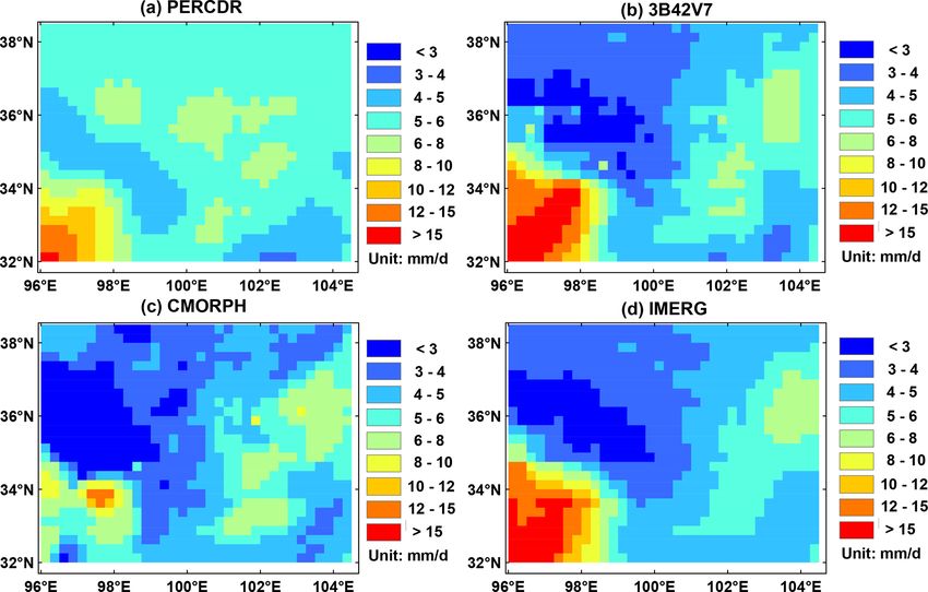
Y. Ma et al.: A two-stage blending approach for merging multiple satellite precipitation estimates                              365

3.3    Error analysis                                              Table 2. Summary of statistical error indices (i.e., RMSE, NMAE,
                                                                   and CC) of the original, bias-corrected, and blended SPEs in two
To assess the performance of the proposed TSB method, sev-         scenarios in the NETP.
eral statistical error indices including the root mean square
error (RMSE), normalized mean absolute error (NMAE), and              Scenarios     Product         RMSE        NMAE       CC
the Pearson’s correlation coefficient (CC) are used in this                                        (mm d−1 )     (%)
study. The specific formulas of these metrics can be found                          PERCDR            7.15       70.2     0.382
below:                                                                              3B42V7            8.56       80.3     0.383
           p                                                                        CMORPH            6.25       60.6     0.556
RMSE = < (Sim − Obs)2 >                                   (21)                      IMERG             6.60       62.9     0.506
            < |Sim − Obs| >                                           Scenario 1    BC-PER            6.00       63.5     0.346
NMAE =                         × 100 %                    (22)                      BC-V7             5.83       61.4     0.408
             P < Obs >                                                              BC-CMO            5.43       56.3     0.533
               [(Sim− < Sim >)(Obs− < Obs >)]                                       BC-IME            5.44       56.0     0.530
CC = pP                          pP                     ,
             (Sim− < Sim > )2        (Obs− < Obs > )2                               Blended SPE       5.36       54.6     0.570
                                                          (23)                      PERCDR            9.19       79.3     0.261
                                                                                    3B42V7            8.38       71.3     0.403
where “Sim” and “Obs” stand for the simulated and observed                          CMORPH            7.20       61.9     0.493
data, respectively; the angle brackets stand for the sample                         IMERG             7.64       65.1     0.462
average.                                                              Scenario 2    BC-PER            7.03       64.5     0.253
                                                                                    BC-V7             6.69       61.3     0.395
                                                                                    BC-CMO            6.41       58.2     0.480
4     Results                                                                       BC-IME            6.44       57.7     0.470
                                                                                    Blended SPE       6.37       56.7     0.513
In the experiment, model parameters are calibrated on the
daily precipitation of warm season in 2014, where GR data
at the 27 black grids in Fig. 1 are randomly selected for train-   zero, which implies a clear effect of elevation on this satel-
ing the model. The model validation is performed under two         lite product. In the data fusion step (Fig. 5), IMERG has the
scenarios: Scenario 1 will validate the model in space based       highest weight and PERCDR has the lowest weight among
on the data of the same period in validation stations (i.e., the   the four bias-corrected SPEs. Moreover, 3B42V7 and PER-
seven red grids in Fig. 1), and Scenario 2 will validate the       CDR have a similar contribution in the blended result. Ba-
model in time based on the data of warm season from 2010           sically, Bayesian analysis is able to simulate the parameter
to 2013 at the same 27 black grids in Fig. 1. In addition,         uncertainty in contrast to traditional statistical methods.
we consider a 10-fold cross-validation in space by randomly
selecting 7 sites for model validation and the data of the re-     4.2     Model validation under two scenarios
maining 27 sites as the training set. The performance of the
TSB approach is further compared with BMA and OOR in               Table 2 presents the summary of the statistical error indices
the two scenarios.                                                 including RMSE, NMAE, and CC of the original (i.e., PER-
                                                                   CDR, 3B42V7, CMORPH and IMERG), bias-corrected (i.e.,
4.1    Parameter estimates                                         BC-PER, BC-V7, BC-CMO, and BC-IME), and blended
                                                                   SPE under two scenarios in the NETP. Subsection 4.2.1
Figures 4 and 5 show the posterior distribution curves of the      and 4.2.2 show the performance of the model validation un-
posterior parameters in Stage 1 and 2, respectively. As for        der Scenario 1 and 2, respectively.
each parameter in the bias-corrected process, the individual
SPEs including PERCDR, 3B42V7, CMORPH, and IMERG                   4.2.1    Scenario 1
show a similar pattern (Fig. 4a to d). This shows that the bias
structures of the original SPEs have similar characteristics.      The original SPEs show large biases, with the RMSE,
For all SPEs, the distribution mass of parameter βi is com-        NMAE, and CC indices ranging from 6.25–8.56 mm d−1 ,
pletely on the right side of zero, which implies that a sys-       60.6 %–80.3 %, and 0.382–0.556, respectively. 3B42V7 has
tematic bias exists for all satellite products. When looking at    the worst skill, with the highest RMSE of 8.56 mm d−1 ,
the effects of elevation, the posterior distribution of parame-    the highest NMAE of 80.3 %, and the second lowest CC
ter γi for PERCDR, 3B42V7, and CMORPH (Fig. 4a–c) has              of 0.383. CMORPH shows the best performance, with the
a value zero in the middle range of the distribution, which        lowest RMSE of 6.25 mm d−1 , the lowest NMAE of 60.6 %,
implies that elevation may have little impact on these three       and the highest CC of 0.556, which presents its superiority
satellite products, while for IMERG in Fig. 4d, the distri-        compared with the other original SPEs in the NETP. Based
bution mass of parameter γi is mostly on the right side of         on the BC model, all the bias-corrected SPEs have better

https://doi.org/10.5194/hess-25-359-2021                                           Hydrol. Earth Syst. Sci., 25, 359–374, 2021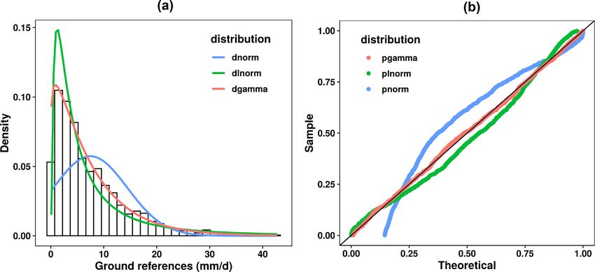
366                    Y. Ma et al.: A two-stage blending approach for merging multiple satellite precipitation estimates

Figure 4. The PDF curves of posterior parameter sets with regard to (a) PERCDR, (b) 3B42V7, (c) CMORPH, and (d) IMERG in the bias
correction process of Stage 1.

                                                                   to GRs in terms of RMSE, NMAE, and CC at 5.36 mm h−1 ,
                                                                   54.6 %, and 0.57, respectively, compared with both the orig-
                                                                   inal and bias-corrected SPEs. The RMSE and NMAE values
                                                                   of the blended SPE decrease by 14.3 %–37.4 % and 10 %–
                                                                   32 %, respectively, and the CC value increases by 2.4 %–
                                                                   49.2 %, accordingly, compared to the original SPEs. In addi-
                                                                   tion, the RMSE, NMAE, and CC of the blended SPE increase
                                                                   by 1.4 %–10.8 %, 2.5 %–14.1 %, and 6.8 %–64.8 %, respec-
                                                                   tively, compared with the bias-corrected SPEs. This proves
                                                                   that the blended SPE exhibits higher quality after Stage 2,
                                                                   due to the ensemble contribution of the bias-corrected SPEs.
                                                                   The relative weight of BC-PER, BC-V7, BC-CMO, and BC-
                                                                   IME is 0.02, 0.038, 0.295, and 0.647, respectively. The BC-
                                                                   IME and BC-PER have the highest and lowest weights, re-
Figure 5. The PDF curves of posterior parameter sets in the data   spectively, and the BC-V7 and BC-CMO rank between BC-
fusion process of Stage 2.                                         IME and BC-PER (Fig. 6a). As for the original SPEs, it is
                                                                   found that there is an overestimation when the rainfall is less
                                                                   than 7.6 mm d−1 and an underestimation when the rainfall
agreement with GRs compared with the original SPEs. Their          is more than 7.6 mm d−1 . Based on the proposed TSB ap-
RMSE scores range from 5.43 to 6 mm d−1 and decrease by            proach, the blended SPE is closer towards the GRs (Fig. 6b
13 %–31.8 %, and their NMAE scores vary from 56.0 % to             and c). Meanwhile, BC-PER seems to be clearly different
63.5 %, and decline by 7.1 % to 23.5 %, respectively. Mean-        from the other bias-corrected SPEs, and up to this point in
while, their CC values range from 0.346 to 0.533 after bias        the study has shown little value for it to be kept in considera-
correction. With the BW model, the blended SPE is closer

Hydrol. Earth Syst. Sci., 25, 359–374, 2021                                          https://doi.org/10.5194/hess-25-359-2021
Y. Ma et al.: A two-stage blending approach for merging multiple satellite precipitation estimates                                   367

tion in the merging process. However, it is worth noting that        Table 3. Summary of the mean values of RMSE, NMAE, and CC
PERCDR can in fact be informative on a case-by-case basis.           for the original and blended SPEs for 10 random verified tests in the
                                                                     warm season of 2014 in the NETP.
4.2.2    Scenario 2
                                                                               Product           RMSE         NMAE        CC
The proposed TSB approach is also validated in Scenario 2,                                      (mm d−1 )      (%)
where the blended SPE shows better performance in terms                        PERCDR              7.96         75.9     0.330
of its RMSE, NMAE, and CC at 6.37 mm h−1 , 56.7 %, and                         3B42V7              7.72         73.8     0.424
0.513, respectively, compared with both the original and                       CMORPH              6.59         63.1     0.520
bias-corrected SPEs. It shows that the original SPEs includ-                   IMERG               6.78         62.7     0.518
ing PERCDR, 3B42V7, CMORPH, and IMERG have high                                Blended SPE         5.75         57.1     0.551
RMSE and NMAE scores in terms of 7.20–9.19 mm h−1 and
61.9 %–79.3 %, respectively, and low CC values in terms
of 0.261–0.493. After the bias correction, the four satellite        4.4   Model comparison with BMA and OOR
products have increased their performance, with lower er-
ror indices than the original SPEs. The RMSE indices of              To assess the performance of the proposed TSB approach,
the bias-corrected SPEs vary from 6.41 to 7.03 mm h−1 , and          it is beneficial to compare the TSB result with the existing
the corresponding NMAE and CC indices are from 57.7 %                fusion approach. In this study, the BMA approach makes use
to 64.5 % and from 0.253 to 0.48, respectively. Based on             of four original satellite data and the corresponding GR data
the data fusion process, the error indices of the blended            at the 27 black grids shown in Fig. 1 in the warm season
SPE including RMSE, NMAE, and CC are 6.37 mm h−1 ,                   of 2014 to estimate the optimal BMA weights. In Scenario 1,
56.7 %, and 0.513, respectively. It is found that the RMSE           the BMA data are calculated based on the BMA weights and
and NMAE values of the blended SPE decreased by 11.5 %–              the original SPEs from the seven red grids in the warm season
30.7 % and 8.4 %–28.5 %, respectively, and the CC value in-          of 2014, and the OOR data are calculated based on the OOR
creases by 4.1 %–96.6 % compared with the original SPEs.             method using the original SPE data from the seven red grids
   As learned from the two validated scenarios, it is proven         in the warm season of 2014. In Scenario 2, the BMA data
that the TSB approach has the potential to improve the satel-        are calculated based on the BMA weights and the original
lite rainfall accuracy, and it has the ability to extract benefits   SPEs from the 27 black grids in the warm season from 2010
from SPEs in terms of higher performances and mitigate poor          to 2013, and the OOR result is calculated based on the OOR
impacts from the ones with lower quality.                            method and the original SPE data from the 27 black grids
                                                                     in the warm season from 2010 to 2013. Herein, we compare
4.3     Cross-validation                                             the blended SPE with both the BMA and OOR predictions in
                                                                     two scenarios, and their statistical error summary is shown in
Figures 7 and 8 show the statistics of evaluation scores of
                                                                     Table 5.
RMSE, NMAE, and CC for the original SPEs and blended
                                                                        In Scenario 1, the TSB method achieves better skill scores,
estimates at the validation grids, with 10 random tests of the
                                                                     with RMSE, NMAE, and CC values of 5.36 mm d−1 , 54.6 %,
gauge locations in the warm season of 2014. For each test,
                                                                     and 0.57, respectively, as compared with the BMA and OOR
seven grid sites are randomly selected from the 34 grid cells
                                                                     approaches. In addition, OOR shows the worst performance
and used for model verification, and the remaining 27 grid
                                                                     in terms of RMSE, NMAE, and CC at 6.22 mm d−1 , 59.7 %,
sites are used for training the model.
                                                                     and 0.537, respectively. BMA shows better skill than OOR
   As for the blended SPE, it achieves similar scores at the
                                                                     but worse skill than TSB, in terms of the RMSE, NMAE,
validation grids among the 10-fold random samples. The
                                                                     and CC values at 5.78 mm d−1 , 56.6 %, and 0.562, respec-
blended SPE shows better skill compared with the origi-
                                                                     tively. In Scenario 2, a similar performance is found for the
nal SPEs for each test in terms of RMSE, NMAE, and CC
                                                                     TSB approach, which has a lower RMSE (6.37 mm d−1 ) and
(Fig. 7). Statistically, the mean values of RMSE, NMAE,
                                                                     NMAE (56.7 %) and higher CC (0.513) than both the OOR
and CC for the blended SPE are 5.75 mm h−1 , 57.1 %,
                                                                     and BMA results. Basically, as compared with the two exist-
and 0.551, respectively (Table 3). The averaged improve-
                                                                     ing fusion algorithms (BMA and OOR) in the two validated
ment ratios of RMSE for the blended SPE are 27.6 %,
                                                                     scenarios, it is confirmed that the TSB method has the advan-
25 %, 10.6 %, and 13 % compared to the PERCDR, 3B42V7,
                                                                     tage of combining the original SPEs and reducing the bias of
CMORPH and IMERG, respectively, and a similar perfor-
                                                                     the satellite precipitation retrievals. It is noted that the daily
mance is seen for NMAE, with average improvement ratios
                                                                     precipitation estimates follow a gamma distribution (Eq. 1)
of 24.5 %, 22.3 %, 7.8 %, and 7.3 %, respectively (Table 4).
                                                                     in this study. In future work it would be interesting to exam-
In summary, the 10-fold cross-validation further verified that
                                                                     ine whether the gamma distribution can be used in the BMA
the blended SPE has a higher accuracy of gridded precipita-
                                                                     algorithm without converting it to a Gaussian distribution.
tion than the original satellite products.

https://doi.org/10.5194/hess-25-359-2021                                              Hydrol. Earth Syst. Sci., 25, 359–374, 2021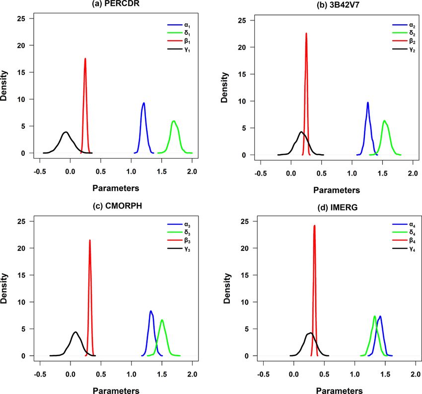
368 Y. Ma et al.: A two-stage blending approach for merging multiple satellite precipitation estimates
Figure 6. (a) The box-and-whisker plots of relative weights for the bias-corrected SPEs, (b) the scatter plots between GRs and the original
SPEs, and (c) the PDF of daily rainfall for the GRs and original and blended SPEs with various rain intensities in Scenario 1 in the NETP.
Table 4. Mean improvement ratios of statistical error indices of the blended SPE, in terms of RMSE, NMAE, and CC compared with the
original SPES for 10 random verified tests in the warm season of 2014 in the NETP.
Index PERCDR 3B42V7 CMORPH IMERG
Improvement RMSE (mm d−1 ) 27.6 25.0 10.6 13.0
ratio (%) NMAE (%) 24.5 22.3 7.8 7.3
CC 71.1 39.8 11.1 10.7
Table 5. Summary of statistical error indices (i.e., RMSE, NMAE, Table 6. Summary of statistical error indices (i.e., RMSE, NMAE,
and CC) for three fusion methods (i.e., OOR, BMA, and TSB) in and CC) for the original and blended SPEs during a heavy rainfall
the two scenarios in the NETP. event of 22 September 2014 in the NETP.
Scenarios Method RMSE NMAE CC Product RMSE NMAE CC
(mm d−1 ) (%) (mm d−1 ) (%)
OOR 6.22 59.7 0.537 PERCDR 8.18 47.0 0.850
Scenario 1 BMA 5.78 56.6 0.562 3B42V7 9.24 52.8 0.683
TSB 5.36 54.6 0.570 CMORPH 8.27 48.5 0.734
OOR 7.04 59.9 0.498 IMERG 8.63 49.1 0.642
Scenario 2 BMA 6.79 58.8 0.500 Blended SPE 5.23 31.5 0.837
TSB 6.37 56.7 0.513
and CMORPH data have a nearly similar contribution in the
blended SPE.
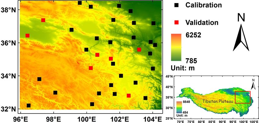
4.5 Model performance on a heavy rainfall case Table 6 reports the evaluation statistics reflecting the
blended performance for this case. It shows that the RMSE,
Local recycling plays a premier role in the moisture sources NMAE, and CC values of the original SPEs range from
of rainfall extremes in the NETP (Ma et al., 2020a). The 8.18–9.24 mm d−1 , 47 %–52.8 %, and 0.642–0.85, respec-
22 September 2014 event was a storm that represents the tively. Compared to the original SPEs, the blended SPE has
local heavy rainfall pattern in the warm season. Consider- a lower RMSE of 5.23 mm d−1 , lower NMAE of 31.5 %,
ing that accurate precipitation estimates for extreme weather and higher CC of 0.837, respectively. The RMSE and
are very important for flood hazard mitigation, we investi- NMAE values of the blended SPE decrease by 36.1 %–
gate the utility of the proposed TSB approach for this event to 43.4 % and 33 %–40.3 %, respectively. The performance
quantify its performance in an extreme rainfall case (Fig. 9a). of the TSB approach is further explored at three gauge
The relative weights of BC-PER, BC-V7, BC-CMO, and BC- cells (i.e., IDs 56171, 56173, 56067), with the top three
IME for the blended SPE are 0.264, 0.14, 0.191, and 0.405, daily rainfall records on 22 September 2014. Figure 10
respectively, for this event (Fig. 9b). It is found that the shows the PDF curves of blended samples at the three
IMERG data have the biggest contribution, and the 3B42V7 sites in this case. It demonstrates that the blended SPE
Hydrol. Earth Syst. Sci., 25, 359–374, 2021 https://doi.org/10.5194/hess-25-359-2021Y. Ma et al.: A two-stage blending approach for merging multiple satellite precipitation estimates 369
Figure 8. The box-and-whisker plots of improvement ratios of
statistics for the blended SPE compared with the original SPEs, in-
cluding PERCDR, 3B42V7, CMORPH, and IMERG for 10 random
verified tests in the warm season of 2014 in the NETP: (a) RMSE,
Figure 7. Statistical error indices of the original and blended SPEs (b) NMAE, and (c) CC.
for 10 random verified tests in the warm season of 2014 in the
NETP: (a) RMSE, (b) NMAE, and (c) CC.
4.6 Model application in a spatial domain
has the advantage in quantifying the predictive uncer- It is important to explore the Bayesian ensembles at unknown
tainty on rainfall extremes at each site. For example, at sites in the domain. As learned from Fig. 11, it seems that
ID 56171, the rainfall estimates that are derived from the each of the original SPEs can capture the spatial pattern of
original SPEs are 19.8 mm (PERCDR), 35.3 mm (3B42V7), daily mean precipitation in the warm season but might fail in
26 mm (CMORPH), and 21.2 mm (IMERG), respec- the representation of the precipitation amount, partly because
tively. 3B42V7 shows an overestimation, while PERCDR, of the satellite retrieval bias in complex terrain and limited
CMORPH, and IMERG underperform the daily rainfall at GR network. Thus, the TSB method is further applied in the
the corresponding pixel (Fig. 10a). Based on the proposed region of interest to demonstrate its performance for daily
TSB approach, the mean value of the merging estimates is precipitation in the warm season of 2010–2014 in the NETP.
28 mm d−1 . At IDs 56173 and 56067, the mean values of It is found that the blended SPE shows high precipitation in
the blended SPE are 26.2 and 19.7 mm d−1 , respectively, the southwest and low precipitation in the northwest, as well
and they are close to GRs with daily amounts of 30.9 and as moderate precipitation in the eastern region. In addition,
28.7 mm, respectively (Fig. 10b and c). Overall, these anal- as compared with the original SPEs, higher values disappear
yses reveal that the TSB algorithm could not only quantify from the spatial map except in the southwest corner for the
its predictive uncertainty, but also improve the daily rainfall blended SPE. The possible reason is that daily mean rain-
amount, even under heavy rainfall conditions. fall is the highest in the southwest corner for most SPEs,
and larger value exists after the TSB approach. Meanwhile,
https://doi.org/10.5194/hess-25-359-2021 Hydrol. Earth Syst. Sci., 25, 359–374, 2021370 Y. Ma et al.: A two-stage blending approach for merging multiple satellite precipitation estimates
Figure 9. (a) Spatial pattern of gauge-based measurements during a heavy rainfall case of 22 September 2014 in the NETP, where the site
IDs 56171, 56173, and 56067 report the top three daily rainfall amounts of 32.3, 30.9, and 28.7 mm, respectively. (b) The corresponding
box-and-whisker plots of relative weights of the bias-corrected SPEs in the data fusion process.
Figure 10. The PDF curves of blended SPE samples and the corresponding mean value at three gauge-based grids for a heavy rainfall case
on 22 September 2014: (a) ID 56171, (b) ID 56173, and (c) ID 56067. The original SPEs and GRs at each pixel are also indicated in each
panel.
the predictive Bayesian uncertainties including lower (2.5 %) required to improve the orographic precipitation in the TP in
and upper (97.5 %) quantiles are displayed from Fig. 12b to c future.
to illustrate the blending variation in this application. The data fusion application is based on four mainstream
SPEs, and BC-IME and BC-PER show the best and worst
performances among the bias-corrected SPEs in Stage 1. It
5 Discussion raises a question as to why the first stage of bias correc-
tion is not simply applied and then the best-performing bias-
In spite of the superior performance of the TSB algorithm, corrected SPE selected as the final product. To address this
some issues still need to be considered in practical applica- issue, we investigate the statistical error differences among
tions, detailed in the following. the BC-IME and blended SPE before and after the removal
Because of limited knowledge on the influences of com- of BC-PER for 10-fold cross validation in the warm season
plex terrain and local climate on the rainfall patterns in the of 2014 in the NETP (Fig. 13). It is beneficial to involve
study area, the elevation feature is considered in the first the Stage 2 in the TSB method because the blended SPE
stage. Table 7 quantifies the impact of the elevation covariate performs better skill than the best-performed bias-corrected
on the bias-corrected and blended SPE performances in Sce- SPE (i.e., BC-IME) in Stage 1. The primary reason is that
nario 1 in the warm season of 2014 in the NETP. It is found the BW model is designed to integrate various types of bias-
that the inclusion of the elevation feature provides slightly corrected SPE, which is limited in the BC model. In addition,
better skill compared with the results without terrain infor- both the blended SPEs with and without the consideration of
mation in this experiment. Considering that deep convective PERCDR show similar performances of the RMSE, NMAE,
systems occurring near the mountainous area have an effect and CC indices (Fig. 13). It implies that the TSB approach
on the precipitation cloud (Houze, 2012), more attempts are
Hydrol. Earth Syst. Sci., 25, 359–374, 2021 https://doi.org/10.5194/hess-25-359-2021Y. Ma et al.: A two-stage blending approach for merging multiple satellite precipitation estimates 371 Figure 11. Spatial patterns of the daily mean precipitation in terms of the original SPEs in the warm season of 2010 to 2014 in the NETP: (a) PERCDR, (b) 3B42V7, (c) CMORPH, and (d) IMERG. Figure 12. Spatial patterns of the blended SPE in terms of (a) mean, (b) lower quantile (2.5 %), and (c) upper quantile (97.5 %) of daily mean precipitation in the warm season of 2010 to 2014 in the NETP. has the advantage of not being impacted by the poor-quality It seems that the performance of the blended SPE becomes individuals (e.g., BC-PER), partly because the BW model similar as the number of training sites increases to 21. We can reallocate the contribution of the bias-corrected SPEs admit that more information from the ground observations based on their corresponding bias characteristics. would be more beneficial for the blended gridded product in In addition, as calculating the blended result at any new the region of interest. It is noted that, if extended to the TP or sites, the model parameters derived from the training grid global scale, the extension of model parameters and training sites are assumed to be applicable in the whole domain. Since sites should be carefully considered. For instance, there are we have a relatively dense GR network in the survey region, few gauges installed in the western and central TP (Ma et al., the current assumption is acceptable according to the perfor- 2015); it might be a potential risk to directly apply this fusion mance of the blended SPE. It is helpful to give some guide- algorithm to these regions. lines on how many training sites are needed to apply the The aim of this study is not to model rainfall processes in a TSB approach in a region with complex terrain and limited target domain but to propose an idea to extract valuable infor- GRs. The sensitivity analysis of the number of training grid mation from available SPEs and provide more reliable grid- cells on the performance of blended SPE at the validation ded precipitation in the high–cold region with complex ter- grids is explored in Fig. 14. As the number of training sites rain. Considering its spatiotemporal differences and the exis- is increasing, there is a decreasing trend for the RMSE and tence of many zero-value records, rainfall is extremely diffi- NMAE values but a slight increasing trend for the CC value. cult to observe and predict (Yong et al., 2015; Bartsotas et al., https://doi.org/10.5194/hess-25-359-2021 Hydrol. Earth Syst. Sci., 25, 359–374, 2021
372                      Y. Ma et al.: A two-stage blending approach for merging multiple satellite precipitation estimates

Table 7. Summary of statistical error indices (i.e., RMSE, NMAE,
and CC) for bias-corrected and blended SPEs with and without con-
sideration of terrain feature as a covariate in the TSB method in
Scenario 1 in the NETP.

     Product        Type          RMSE       NMAE        CC
                                 (mm d−1 )    (%)
                    No terrain     5.98        63.3     0.361
     BC-PER
                    Terrain        6.00        63.5     0.346
                    No terrain     5.83        61.5     0.409
     BC-V7
                    Terrain        5.83        61.4     0.408
                    No terrain     5.48        56.9     0.520
     BC-CMO
                    Terrain        5.43        56.3     0.533
                    No terrain     5.48        56.3     0.519
     BC-IME
                    Terrain        5.44        56.0     0.530
                    No terrain     5.41        55.0     0.557
     Blended SPE
                    Terrain        5.36        54.6     0.570

2018). With regard to the probability of rainfall occurrence,
a zero-inflated model, which is coherent with the empirical
distribution of rainfall amount, is expected to improve the
proposed TSB algorithm. Also, hourly or even instantaneous
precipitation intensity is extremely vital for flood prediction,
which should be specifically designed when extending this
fusion framework in the next step.

6    Summary and prospects
                                                                    Figure 13. Statistical error indices (i.e., RMSE, NMAE, and CC)
This study proposes a TSB algorithm for multi-SPE data fu-          of the best-performing bias-corrected SPE (i.e., BC-IME, black)
sion. A preliminary experiment is conducted in the NETP             and blended SPE before (red) and after (blue) removing the worst-
using four mainstream SPEs (i.e., PERCDR, 3B42V7,                   performing BC-PER, for 10 random verified tests in the warm sea-
CMORPH, and IMERG) to demonstrate the performance of                son of 2014 in the NETP.
this TSB approach. Primary conclusions are summarized be-
low:

    1. This TSB algorithm has two stages and involves the
       BC and BW models. It is found that this blended method
       is capable of involving a group of original SPEs. Mean-
       while, it provides a convenient way to quantify the fu-
       sion performance and the associated uncertainty.

    2. The experiment shows that the blended SPE has bet-
       ter skill scores compared to the original SPEs in the two
       validated scenarios. The 10-fold cross validation in Sce-
       nario 1 further confirms the superiority of the TSB al-
       gorithm. In addition, it is found that the TSB method
       outperforms another two existing fusion methods (i.e.,       Figure 14. Statistical error indices (i.e., RMSE, NMAE, and CC)
       BMA and OOR) in the two scenarios. The performance           of the blended SPE at the validation grid locations in terms of a
       of this fusion method is also demonstrated for a heavy       different number of training sites in the warm season of 2014 in
       rainfall event in the region of interest.                    the NETP.

Hydrol. Earth Syst. Sci., 25, 359–374, 2021                                           https://doi.org/10.5194/hess-25-359-2021
Y. Ma et al.: A two-stage blending approach for merging multiple satellite precipitation estimates 373
3. The application proves that this algorithm can allocate References
the contribution of individual SPEs to the blended re-
sult because it is capable of ingesting useful informa-
tion from uneven individuals and alleviating potential Ashouri, H., Hsu, K. L., Sorooshian, S., Braithwaite, D. K., Knapp,
K. R., Cecil, L. D., Nelson, B. R., and Prat O. P.: PERSIANN-
negative impacts from the poorly performing members.
CDR: Daily Precipitation Climate Data Record from Multisatel-
Overall, this work provides an opportunity for merging SPEs lite Observations for Hydrological and Climate Studies, B. Am.
in the high–cold region with complex terrain. The evaluation Meteorol. Soc., 96, 69–83, 2015.
Baez-Villanueva, O. M., Zambrano-Bigiarini, M., Beck, H. E.,
analysis of this TSB method for extended regions (e.g., TP)
McNamara, I., Ribbe, L., Nauditt, A., Birkel, C., Verbist, K.,
in terms of higher temporal resolution (e.g., hourly) will be
Giraldo-Osorio, J. D., and Thinh, N. X.: RF-MEP: A novel Ran-
performed in a future study. dom Forest method for merging gridded precipitation products
and ground-based measurements, Remote Sens. Environ., 239,
111606, https://doi.org/10.1016/j.rse.2019.111606, 2020.
Data availability. The gauge data are from the China Meteoro- Bartsotas, N. S., Anagnostou, E. N., Nikolopoulos, E. I., and Kallos,
logical Data Service Center (http://data.cma.cn, last access: Jan- G.: Investigating satellite precipitation uncertainty over complex
uary 2021). The PERCDR data are from http://www.ncei.noaa.gov/ terrain, J. Geophys. Res.-Atmos., 123, 5346–5369, 2018.
data/precipitation-persiann/ (last access: January 2021) (Ashouri Beck, H. E., van Dijk, A. I. J. M., Levizzani, V., Schellekens,
et al., 2015). The CMORPH data are from https://rda.ucar.edu/ J., Miralles, D. G., Martens, B., and de Roo, A.: MSWEP: 3-
datasets/ds502.2/ (last access: January 2021) (Xie et al., 2017). The hourly 0.25◦ global gridded precipitation (1979–2015) by merg-
3B42V7 data are from https://disc2.gesdisc.eosdis.nasa.gov/data/ ing gauge, satellite, and reanalysis data, Hydrol. Earth Syst. Sci.,
TRMM_L3/TRMM_3B42_Daily.7/ (last access: January 2021) 21, 589–615, https://doi.org/10.5194/hess-21-589-2017, 2017.
(Huffman et al., 2007). The IMERG data are from https://gpm1. Cuo, L., Zhang, Y., Gao, Y., Hao, Z., and Cairang, L.: The impacts
gesdisc.eosdis.nasa.gov/data/GPM_L3/GPM_3IMERGDF.06/ (last of climate change and land cover/use transition on the hydrology
access: January 2021) (Huffman et al., 2018). in the upper Yellow River Basin, China, J. Hydrol., 502, 37–52,
2013.
Derin, Y., Anagnostou, E., Berne, A., Borga, M., Boudevillain, B.,
Author contributions. YM and XS conceived the idea. XS and Buytaert, W., Chang, C., Chen, H., Deirieu, G., Hsu, Y., Lavado-
YZ acquired the project and financial support. YM conducted the Casimiro, W., Manz, B., Moges, S., Nikolopoulos, E., Sahlu,
detailed analysis. HC, XS, and YZ gave comments on the analysis. D., Salerno, F., Rodriguez-Sanchez, J., Vergara, H., and Yilmaz,
All the authors contributed to the writing and revisions. K.: Evaluation of GPM-era global satellite precipitation products
over multiple complex terrain regions, Remote Sens., 11, 2936,
https://doi.org/10.3390/rs11242936, 2019.
Competing interests. The authors declare that they have no conflict Gelman, A., Carlin, J. B., Stern, H. S., Dunson, D. B., Vehtari,
of interest. A., and Rubin, D. B.: Bayesian Data Analysis-Third Edition,
CPC Press, New York, 2013.
Hou, A. Y., Kakar, R. K., Neeck, S., Azarbarzin, A. A., Kummerow,
Financial support. This study is supported by the National Key Re- C. D., Kojima, M., Oki, R., Nakamura, K., and Iguchi, T.: The
search and Development Program of China (nos. 2017YFC1503001 Global Precipitation Measurement Mission, B. Am. Meteorol.
and 2017YFA0603101) and the Strategic Priority Research Pro- Soc., 95, 701–722, 2014.
gram (A) of CAS (no. XDA2006020102). Houze, R. A.: Orographic effects on precipitating clouds, Rev.
Geophys., 50, RG1001, https://doi.org/10.1029/2011RG000365,
2012.
Huffman, G., Adler, R., Arkin, P., Chang, A., Ferraro, R., Gruber,
Review statement. This paper was edited by Fuqiang Tian and re-
A., Janowiak, J. E., McNab, A., Rudolf, B., and Schneider, U.:
viewed by three anonymous referees.
The global precipitation climatology project (GPCP) combined
precipitation dataset, B. Am. Meteorol. Soc., 78, 5–20, 1997.
Huffman, G. J., Bolvin, D. T., Nelkin, E. J., Wolff, D. B., Adler,
R. F., Gu, G., Hong, Y., Bowman, K. P., and Stocker E. F.: The
TRMM Multisatellite Precipitation Analysis (TMPA): quasi-
global, multiyear, combined-sensor precipitation estimates at
fine scales, J. Hydrometeorol., 8, 38–55, 2007.
Huffman, G. J., Bolvin, D. T., Braithwaite, D., Hsu, K., Joyce,
R., Kidd, C., Nelkin, E. J., Sorooshian, S., Tan, J., and Xie,
P.: NASA Global Precipitation Measurement (GPM) Integrated
Multi-satellitE Retrievals for GPM (IMERG), Algorithm The-
oretical Basis Document (ATBD) Version 5.2, NASA/GSFC,
Greenbelt, MD, USA, 2018.
Joyce, R. J., Janowiak, J. E., Arkin, P. A., and Xie, P.: CMORPH: A
method that produces global precipitation estimates from passive
https://doi.org/10.5194/hess-25-359-2021 Hydrol. Earth Syst. Sci., 25, 359–374, 2021374 Y. Ma et al.: A two-stage blending approach for merging multiple satellite precipitation estimates microwave and infrared data at high spatial and temporal resolu- Robertson, D. E., Shrestha, D. L., and Wang, Q. J.: Post-processing tion, J. Hydrometeorol., 5, 487–503, 2004. rainfall forecasts from numerical weather prediction models for Krajewski, W. F.: Cokriging radar-rainfall and rain gage data, J. short-term streamflow forecasting, Hydrol. Earth Syst. Sci., 17, Geophys. Res., 92, 9571–9580, 1987. 3587–3603, https://doi.org/10.5194/hess-17-3587-2013, 2013. Li, H., Hong, Y., Xie, P., Gao, J., Niu, Z., Kirstetter, P. E., and Yong, Shen, Y. and Xiong, A.: Validation and comparison of a new gauge- B.: Variational merged of hourly gauge-satellite precipitation in based precipitation analysis over mainland China, Int. J. Clima- China: preliminary results, J. Geophys. Res.-Atmos., 120, 9897– tol., 36, 252–265, 2016. 9915, 2015. Shen, Y., Xiong, A., Hong, Y., Yu, J., Pan, Y., Chen, Z., and Sa- Ma, Y. and Chandrasekar, V.: A Hierarchical Bayesian Ap- haria, M.: Uncertainty analysis of five satellite-based precipita- proach for Bias Correction of NEXRAD Dual-Polarization tion products and evaluation of three optimally merged multi- Rainfall Estimates: Case Study on Hurricane Irma in algorithm products over the Tibetan Plateau, Int. J. Remote Sens., Florida, IEEE Geosci. Remote Sens. Lett., 99, 1–5, 35, 6843–6858, 2014. https://doi.org/10.1109/LGRS.2020.2983041, 2020. Shrestha, D. L., Robertson, D. E., Bennett, J. C., and Wang, Q. Ma, Y., Zhang, Y., Yang, D., and Farhan S. B.: Precipitation bias J.: Improving Precipitation Forecasts by Generating Ensembles variability versus various gauges under different climatic condi- through Postprocessing, Mon. Weather Rev., 143, 3642–3663, tions over the Third Pole Environment (TPE) region, Int. J. Cli- 2015. matol., 35, 1201–1211, 2015. Tang, Y., Yang, X., Zhang, W., and Zhang, G.: Radar and Ma, Y., Tang, G., Long, D., Yong, B., Zhong, L., Wan, Rain Gauge Merging-Based Precipitation Estimation via W., and Hong, Y.: Similarity and error intercomparison of Geographical-Temporal Attention Continuous Conditional Ran- the GPM and its predecessor-TRMM Multi-satellite Pre- dom Field, IEEE T. Geosci. Remote, 56, 1–14, 2018. cipitation Analysis using the best available hourly gauge Verdin, A., Rajagopalan, B., Kleiber, W., and Funk, C.: A Bayesian network over the Tibetan Plateau, Remote Sens., 8, 569, kriging approach for blending satellite and ground precipitation https://doi.org/10.3390/rs8070569, 2016. observations, Water Resour. Res., 51, 908–921, 2015. Ma, Y., Hong, Y., Chen, Y., Yang, Y., Tang, G., Yao, Y., Long, D., Xie, P. and Arkin, P.: Global precipitation: a 17-year monthly analy- Li, C., Han, Z., and Liu, R.: Performance of optimally merged sis based on gauge observations, satellite estimates, and numeri- multisatellite precipitation products using the dynamic Bayesian cal model outputs, B. Am. Meteorol. Soc., 78, 2539–2558, 1997. model averaging scheme over the Tibetan Plateau, J. Geophys. Xie, P. and Xiong, A.-Y.: A conceptual model for con- Res.-Atmos., 123, 814–834, 2018. structing high-resolution gaugesatellite merged precipi- Ma, Y., Lu, M., Bracken, C., and Chen, H.: Spatially coher- tation analyses, J. Geophys. Res.-Atmos. 116, D21106, ent clusters of summer precipitation extremes in the Tibetan https://doi.org/10.1029/2011JD016118, 2011. Plateau: Where is the moisture from?, Atmos. Res., 237, 104841, Xie, P., Joyce, S., Wu, S., Yoo, S., Yarosh, Y., Sun, F., and Lin, R.: https://doi.org/10.1016/j.atmosres.2020.104841, 2020a. Reprocessed, bias-corrected CMORPH global high-resolution Ma, Y., Chandrasekar, V., and Biswas, S. K.: A Bayesian correc- precipitation estimates from 1998, J. Hydrometeorol., 18, 1617– tion approach for improving dual-frequency precipitation radar 1641, 2017. rainfall rate estimates, J. Meteorol. Soc. Jpn., 98, 511–525, Yang, Z., Hsu, K., Sorooshian, S., Xu, X., Braithwaite, D., Zhang, https://doi.org/10.2151/jmsj.2020-025, 2020b. Y., and Verbist, K. M. J.: Merging high-resolution satellite-based Prat, O. P. and Nelson, B. R.: Evaluation of precipitation estimates precipitation fields and point-scale rain gauge measurements – a over CONUS derived from satellite, radar, and rain gauge data case study in Chile, J. Geophys. Res.-Atmos., 122, 5267–5284, sets at daily to annual scales (2002–2012), Hydrol. Earth Syst. 2017. Sci., 19, 2037–2056, https://doi.org/10.5194/hess-19-2037-2015, Yong, B., Liu, D., Gourley, J. J., Tian, Y., Huffman, G. J., Ren, 2015. L., and Hong, Y.: Global View Of Real-Time Trmm Multisatel- Renard, B.: A Bayesian hierarchical approach to regional lite Precipitation Analysis: Implications For Its Successor Global frequency analysis, Water Resour. Res., 47, W11513, Precipitation Measurement Mission, B. Am. Meteorol. Soc., 96, https://doi.org/10.1029/2010WR010089, 2011. 283–296, 2015. Hydrol. Earth Syst. Sci., 25, 359–374, 2021 https://doi.org/10.5194/hess-25-359-2021
You can also read