RainBench: Enabling Data-Driven Precipitation Forecasting on a Global Scale
←
→
Page content transcription
If your browser does not render page correctly, please read the page content below
RainBench: Enabling Data-Driven
               Precipitation Forecasting on a Global Scale

                      Catherine Tong∗                      Christian Schroeder de Witt∗
                     University of Oxford                     University of Oxford

    Valentina Zantedeschi         Daniele De Martini       Alfredo Kalaitzis       Matthew Chantry
     GE Global Research           University of Oxford    University of Oxford     University of Oxford

                       Duncan Watson-Parris                          Piotr Biliński
                        University of Oxford                      University of Warsaw

                                                  Abstract

              Climate change is expected to aggravate extreme precipitation events, directly
              impacting the livelihood of millions. Without a global precipitation forecasting
              system in place, many regions – especially those constrained in resources to collect
              expensive groundstation data – are left behind. To mitigate such unequal reach
              of climate change, a solution is to alleviate the reliance on numerical models
              (and by extension groundstation data) by enabling machine-learning-based global
              forecasts from satellite imagery. Though prior works exist in regional precipitation
              nowcasting, there lacks work in global, medium-term precipitation forecasting.
              Importantly, a common, accessible baseline for meaningful comparison is absent.
              In this work, we present RainBench, a multi-modal benchmark dataset dedicated
              to advancing global precipitation forecasting. We establish baseline tasks and
              release PyRain, a data-handling pipeline to enable efficient processing of decades-
              worth of data by any modeling framework. Whilst our work serves as a basis for
              a new chapter on global precipitation forecast from satellite imagery, the greater
              promise lies in the community joining forces to use our released datasets and tools
              in developing machine learning approaches to tackle this important challenge.

1        Introduction
Extreme precipitation events, such as violent rain and hail storms, can devastate crop fields and
disrupt harvests [12, 22]. Although these events can be locally forecasted with sophisticated numerical
weather models that rely on extensive ground and satellite observations, such approaches require
access to compute and data resources that developing countries in need – particularly in South
America and West Africa – cannot afford [5, 11]. The lack of advance planning for precipitation
events impedes socioeconomic development and ultimately affects the livelihoods of millions around
the world. Given the increase in global precipitation and extreme precipitation events driven by
climate change [6], the need for accurate precipitation forecasts is ever more pressing.
To mitigate such unequal reach of climate change, a solution is to alleviate the reliance on numerical
models (and by extension ground-station data) by enabling machine-learning-based forecasts from
global satellite imagery. Several notable prior works exist in applying machine learning techniques to
precipitation forecasting. Early work by Xingjian et al. [24] proposed a convolutional recurrent neural
     ∗
         Equal contributions.

AI for Earth Sciences Workshop at NeurIPS 2020.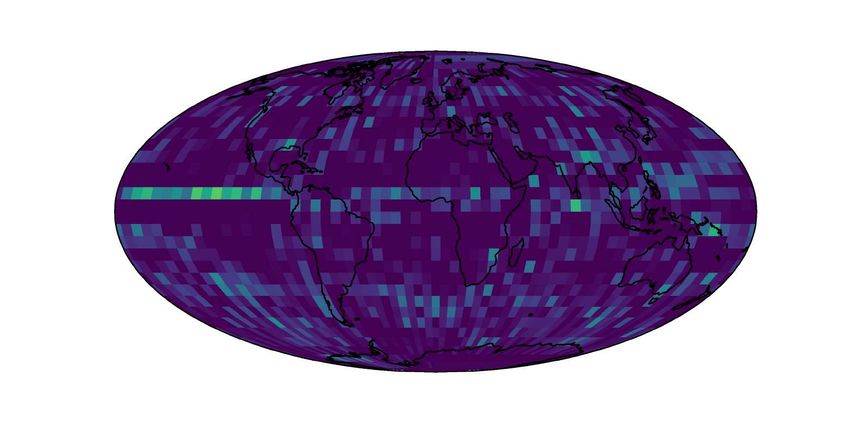
network for precipitation nowcasting. Most recently, Sønderby et al. [21] proposed a “(weather)-
model-free" approach, MetNet, which forecasts precipitation in continental USA using geostationary
satellite images and radar measurements as inputs. This approach performs well up to 7-8 hours, but
inevitably runs into a forecast horizon limit as information from global or surrounding geographic
areas is not incorporated into the system. Such short time windows do not enable substantial disaster
preparedness for disadvantaged populations. Moreover, there lacks a common and accessible dataset
for meaningful comparison in global precipitation forecasting research.
Most related to our work, Rasp et al. [17] developed WeatherBench, a benchmark suite for global
data-driven medium-range weather forecasting. Although WeatherBench forms an excellent first
step in weather forecasting (focusing on temperature and geopotential), it falls short at enabling
precipitation forecasts. First, WeatherBench does not include any observational raw data (e.g. satellite
imagery) and only contains ERA5 precipitation data, which has limited skill in representing extreme
precipitation events. Further, WeatherBench does not include a fast dataloading pipeline to train ML
models, which has been found to be a significant bottleneck in our model development.
In this work, we present RainBench, a multi-modal benchmark dataset dedicated to advancing global
precipitation forecasting. We establish baseline end-to-end forecasting tasks covering realistic data
conditions. Together with the release of an efficient data-handling pipeline, PyRain, we are hopeful
that this work will facilitate future machine learning research in tackling the important challenge of
precipitation forecasting.

2   RainBench
We introduce RainBench a dataset to facilitate research efforts into global precipitation forecasting
from satellite imagery. RainBench results from the combination of the following sources of data.

SimSat. We integrate Simulated Satellite (SimSat) data to minimize data processing requirements
and to simplify the prediction task. SimSat data is model-simulated satellite data generated from Euro-
pean Centre for Medium-Range Weather Forecasts (ECWMF)’s high-resolution weather-forecasting
model using the RTTOV radiative transfer model [20]. SimSat emulates three spectral channels from
the Meteosat-10 SEVIRI satellite [1]. SimSat provides information about global cloud cover and
moisture features and has a native spatial resolution of about 0.1◦ – i.e. about 10 km – at three-hourly
intervals. The product is available from April 2016 to present (with a lag time of 24 h). Using real
satellite data adds unnecessary complication which deviates from the core precipitation forecasting
problem (e.g. the need to account for instrument error and missing values) and is left as future work.

IMERG. We use Integrated Multi-satellitE Retrievals (IMERG), a global half-hourly precipitation
estimation product provided by NASA [8]. Specifically we use the Final Run product which primarily
uses satellite data from multiple polar-orbiting and geo-stationary satellites. This estimate is then
corrected using data from reanalysis products (MERRA2, ERA5) and rain-gauge data. IMERG is
produced at a spatial resolution of 0.1◦ – about 10 km – and is available from June 2000 to present,
with a lag time of about three to four months.

ERA5. As an alternate source of precipitation estimates, we use the ERA5 Reanalysis Product [7]
which provides a global hourly estimate. Additionally, we include the broad spectrum of physical and
atmospheric variables provided in ERA5, such as specific humidity, temperature and geopotential
height at different pressure levels. Estimates cover the full globe at a spatial resolution of 0.25◦ and
are available from 1979 to present, with a lag time of five days.
Alongside RainBench, we release PyRain, an out-of-the-box experimentation framework to make
our released dataset as user-friendly as possible2 . While being optimised for use with RainBench,
PyRain is also compatible with the WeatherBench. PyRain is based on NumPy memmap arrays3 with
optimised software-side access patterns. Empirically we have found this to accelerate data-reading
operations by as much as 60 times when compared to a conventional NetCDF+Dask 4 [18] dataloader.
    2
      Dataloading limitations have been previously identified as a decisive bottleneck by the Pangeo community
in https://pangeo.io/index.html
    3
      https://docs.python.org/3/library/mmap.html (2021)
    4
      https://www.unidata.ucar.edu/software/netcdf/ (2021)

                                                      2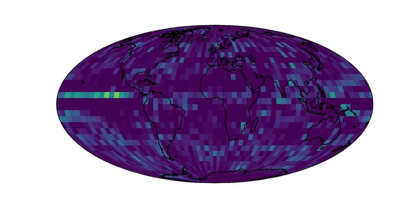
Table 1: Precipitation forecasts evaluated with Latitude-weighted RMSE (mm). All rows except
the last show models trained with data from 2016 onwards. ERA* uses data from 1979 and 2000
onwards for predicting ERA5 and IMERG precipitation respectively. Best results (except ERA*) are
shown in bold.
                                        ERA5                       IMERG
                               1-day     3-day    5-day    1-day    3-day     5-day
             Persistence        0.6249    0.6460     0.6492    1.1321    1.1497     1.1518
             Climatology        0.4798    0.4802     0.4803    0.8244    0.8249     0.8246
             SimSat             0.4610    0.4678     0.4691    0.8166    0.8201     0.8198
             ERA                0.4562    0.4655     0.4677    0.8182    0.8224     0.8215
             SimSat + ERA       0.4557    0.4655     0.4675    0.8134    0.8185     0.8185
             ERA*               0.4485    0.4670     0.4699    0.8085    0.8194     0.8214

2.1   Benchmark Tasks

We define two benchmark tasks on RainBench for precipitation forecasting, with the ground truth
precipitation values taken from either ERA5 or IMERG. For each benchmark task, we consider
three different input data settings: SimSat, reanalysis data (ERA5), or both. When using input data
from ERA5, we use 17 atmospheric state variables that we determine as useful for precipitation
reconstruction through correlation analysis and domain knowledge. Additionally, we use 5 static
variables describing the location and surface of the Earth. We normalize each variable with its global
mean and standard deviation.
We use Convolutional LSTMs [24] as the neural model baseline and structure our forecasting task
based on MetNet’s configurations [21], where a single model is capable of forecasting at different
lead times. Specifically, the network’s input is a time series of features from t = −T to t = 0, and
the output is a precipitation forecast at lead time t = τ . The input time series is a concatenation of
the aforementioned temporal features, static features, time features and a one-hot lead-time vector.
We provide more details in Appendix E.
The tasks are approached as a regression problem. Following [17], we use the mean latitude-weighted
Root-Mean Squared Error (RMSE) as loss and evaluation metric. This is a meaningful metric for
precipitation forecasts as it corrects the oversampling of locations at higher latitudes caused by
degree-based resolutions. We compare the results to two common baselines in weather forecasting
(1) a persistence forecast in which the precipitation at t = 0 is used as prediction at t = τ , and (2) a
climatology forecast in which the mean precipitation in the training data is used as prediction.

3     Benchmarks and Experiments

3.1   Precipitation Forecasting

Table 1 shows our neural model baseline for the two benchmark forecasting tasks.
When predicting ERA5 precipitation, all neural results outperform baselines. Training from SimSat
alone gives the worst results across all data settings. This confirms the difficulty in precipitation
forecast from satellite data alone, which does not contain as much information about the atmospheric
state as sophisticated reanalysis data such as ERA5. Importantly, the complementary benefits of
utilizing data from both sources is already visible despite our simple concatenation setup, as training
from both SimSat and ERA5 achieves the best results across all lead times (when holding the number
of training instances constant).
When predicting IMERG precipitation, the similar performance between the climatology baseline
and neural model suggests that this is a considerably more difficult task. Forecasting skill based
on ERA5 input is only mildly better than the climatology baselines for 1-day and 3-day forecasts.
Upon inspection we found IMERG to feature a longer tail distribution of extreme precipitation events
(Appendix B), which contributes to the increased difficulty of the task.

                                                   3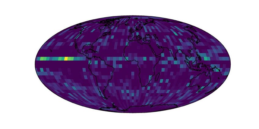
Table 2: Same-timestep estimation of IMERG precipitation with and without balanced sampling,
reported in RMSE. Best results are shown in bold.
                                   Slight Moderate Heavy Violent Micro Avg. Macro Avg.
                  ERA               0.20       4.08      16.2      63.1        0.65          20.9
 Unbalanced       SimSat            0.20       4.38      16.8      54.1        0.65          18.9
                  SimSat + ERA      0.20       4.03      16.5      53.0        0.65          18.4
                  ERA               1.05       2.75      12.4      58.0        1.40          18.6
 Balanced         SimSat            1.17       3.10      13.3      50.1        1.26          16.9
                  SimSat + ERA      1.30       3.15      11.8      44.3        1.38          15.1

We also see the importance in using a larger training dataset, since extending the considered training
instances to the full ERA5 dataset outperforms the baselines further in the 1-day forecasting regime
(shown in the last rows). A key limitation in the baseline setup is that only the overlapping time
frames (from 2016 onwards) of ERA5, IMERG and SimSat are used. This suggests that there is still
significant room for improvement above the presented baselines, especially by developing alternative
modeling setups that adequately make use of the full available data from each source.

3.2   Balanced Sampling Approach

To better understand the challenges posed by an imbalanced occurrence of precipitation events,
we carried out a separate analysis focusing on same-timestep precipitation estimation on IMERG.
We adopted a balanced-sampling approach and measured its effect on model performance in four
precipitation classes (defined according to [15]).
For this analysis, we use LightGBM methods [10]. We use 1 million randomly-sampled pixels
as training data, and compare the (not latitude-adjusted) RMSE for two pixel sampling variants.
A) unbalanced sampling, meaning grid points are chosen randomly from the raw data distribution
and B) balanced sampling, in which we bin IMERG precipitation into four classes and sample grid
points until there is an equal amount of pixels per bin.
In Table 2, we find that balanced sampling reduces the per-class validation RMSE of moderate, heavy
and violent precipitation, resulting in improved macro-averaged RMSE. However, the micro-averaged
RMSE increases due to worsen performance on the ‘Slight Rain’ class, which dominates the dataset
(detailed in Appendix B)

4     Discussion
Designing an appropriate class-balanced sampling may play a crucial role towards improving predic-
tions of extreme precipitation events, a potential solution may lie in a mixture of pixelwise-weighting
and balanced sampling strategies. A closely related issue is data normalization, where a more sophis-
ticated feature scaling approach should be developed to account for any local weather patterns and
spatial differences, such as the Local Area-wise Standardization (LAS) approach proposed in [4].
We suggest refining LAS and adjust the kernel size with latitude, such that the spatial normalization
context remains constant over the globe.
Further, the spherical input and output data topology of global forecasting contexts poses interesting
questions regarding the choice of neural network architectures. While a multitude of approaches to
handle spherical input topologies has been suggested (see [13] for an overview), it seems yet unclear
which approach works best. Our dataset might constitute a valuable benchmark for such research.
Beyond improving upon the proposed benchmark forecasting tasks, RainBench also enables other
exciting research avenues. The availability of a comprehensive list of atmospheric state variables in
RainBench makes feasible a physics-informed learning approach, for instance by taking a multi-task
learning approach to forecast precipitation while simulating physical state variables. Apart from
this, developing approaches which allow for effective use of high-resolution data might provide
performance gains due to the increased amount of information captured, for example by taking a
multi-fidelity approach [9] or by incorporating a local high-resolution model [3]. Investigating a

                                                  4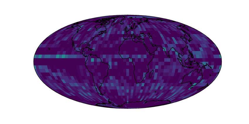
multi-time-step loss function to train the forecast model is another possible approach to improving
generalization performance [14, 2, 23]. Lastly, a local encoder network may be build to provide
low-dimensional embeddings, which could then be fed into a late fusion network architecture
similar to Rudner et al. [19, Multi3 Net]; this might reduce the time lag in obtaining an Early-Run
IMERG product, which is currently constrained by the resource-heavy transfer of high-dimensional
observational data.

Acknowledgements
This research was conducted at the Frontier Development Lab (FDL), Europe. The authors gratefully
acknowledge support from the European Space Agency ESRIN Phi Lab, Trillium Technologies,
NVIDIA Corporation, Google Cloud, and SCAN. The authors are thankful to Peter Dueben, Stephan
Rasp, Julien Brajard and Bertrand Le Saux for useful suggestions.

                                                5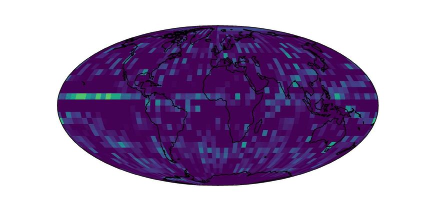
References
 [1] DMA Aminou. Msg’s seviri instrument. ESA Bulletin(0376-4265), (111):15–17, 2002.
 [2] N. D. Brenowitz and C. S. Bretherton. Prognostic Validation of a Neural Network Unified
     Physics Parameterization. Geophysical Research Letters, 45(12):6289–6298, 2018. ISSN
     1944-8007. doi: 10.1029/2018GL078510.
 [3] Gabriele Franch, Valerio Maggio, Luca Coviello, Marta Pendesini, Giuseppe Jurman, and
     Cesare Furlanello. TAASRAD19, a high-resolution weather radar reflectivity dataset for
     precipitation nowcasting. Scientific Data, 7(1):234, July 2020. ISSN 2052-4463. doi: 10.1038/
     s41597-020-0574-8. URL https://www.nature.com/articles/s41597-020-0574-8.
     Number: 1 Publisher: Nature Publishing Group.
 [4] Peter Grönquist, Chengyuan Yao, Tal Ben-Nun, Nikoli Dryden, Peter Dueben, Shigang Li, and
     Torsten Hoefler. Deep Learning for Post-Processing Ensemble Weather Forecasts, May 2020.
 [5] S Gubler, K Sedlmeier, J Bhend, G Avalos, CAS Coelho, Y Escajadillo, M Jacques-Coper,
     R Martinez, C Schwierz, M de Skansi, et al. Assessment of ecmwf seas5 seasonal forecast
     performance over south america. Weather and Forecasting, 35(2):561–584, 2020.
 [6] Aman Kumar Gupta, Dipak Yadav, Priyanka Gupta, Supriya Ranjan, Vishal Gupta, and Sirpat
     Badhai. Effects of climate change on agriculture. Food and Agriculture Spectrum Journal, 1(3),
     2020.
 [7] Hans Hersbach, Bill Bell, Paul Berrisford, Shoji Hirahara, András Horányi, Joaquín Muñoz-
     Sabater, Julien Nicolas, Carole Peubey, Raluca Radu, Dinand Schepers, et al. The era5 global
     reanalysis. Quarterly Journal of the Royal Meteorological Society, 146(730):1999–2049, 2020.
 [8] G.J. Huffman, E.F. Stocker, D.T. Bolvin, E.J. Nelkin, and Jackson Tan. Gpm imerg final
     precipitation l3 half hourly 0.1 degree x 0.1 degree v06. Technical report, 2019.
 [9] Nagoor Kani Jabarullah Khan and Ahmed H. Elsheikh. A Machine Learning Based Hybrid
     Multi-Fidelity Multi-Level Monte Carlo Method for Uncertainty Quantification. Frontiers in
     Environmental Science, 7, 2019. ISSN 2296-665X. Publisher: Frontiers.
[10] Guolin Ke, Qi Meng, Thomas Finley, Taifeng Wang, Wei Chen, Weidong Ma, Qiwei Ye, and
     Tie-Yan Liu. Lightgbm: A highly efficient gradient boosting decision tree. In Advances in
     neural information processing systems, pages 3146–3154, 2017.
[11] Camille Le Coz and Nick van de Giesen. Comparison of rainfall products over sub-saharan
     africa. Journal of Hydrometeorology, 21(4):553–596, 2020.
[12] Yan Li, Kaiyu Guan, Gary D. Schnitkey, Evan DeLucia, and Bin Peng. Excessive rainfall leads
     to maize yield loss of a comparable magnitude to extreme drought in the United States. Global
     Change Biology, 25(7):2325–2337, 2019. ISSN 1365-2486.
[13] Iciar Llorens Jover. Geometric deep learning for medium-range weather prediction, June 2020.
     URL https://infoscience.epfl.ch/record/278138. Master’s Thesis.
[14] J. McGibbon and C. S. Bretherton. Single-Column Emulation of Reanalysis of the Northeast
     Pacific Marine Boundary Layer. Geophysical Research Letters, 46(16):10053–10060, 2019.
     ISSN 1944-8007. doi: 10.1029/2019GL083646.
[15] MetOffice. Fact sheet 3 — Water in the atmosphere. Technical report, MetOffice
     UK, 2012.     URL https://www.metoffice.gov.uk/binaries/content/assets/
     metofficegovuk/pdf/research/library-and-archive/library/publications/
     factsheets/factsheet_3-water-in-the-atmosphere.pdf.
[16] Adam Paszke, Sam Gross, Francisco Massa, Adam Lerer, James Bradbury, Gregory Chanan,
     Trevor Killeen, Zeming Lin, Natalia Gimelshein, Luca Antiga, Alban Desmaison, Andreas
     Kopf, Edward Yang, Zachary DeVito, Martin Raison, Alykhan Tejani, Sasank Chilamkurthy,
     Benoit Steiner, Lu Fang, Junjie Bai, and Soumith Chintala. Pytorch: An imperative style, high-
     performance deep learning library. In H. Wallach, H. Larochelle, A. Beygelzimer, F. d. Alché-
     Buc, E. Fox, and R. Garnett, editors, Advances in Neural Information Processing Systems 32,
     pages 8024–8035. Curran Associates, Inc., 2019.

                                                6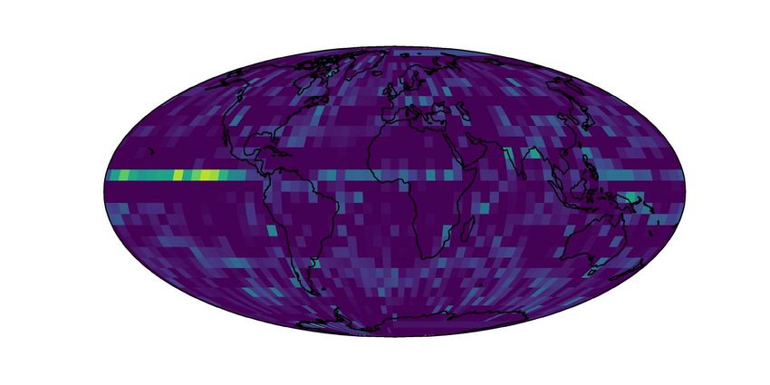
[17] Stephan Rasp, Peter D. Dueben, Sebastian Scher, Jonathan A. Weyn, Soukayna Mouatadid,
     and Nils Thuerey. WeatherBench: A benchmark dataset for data-driven weather forecasting.
     arXiv:2002.00469 [physics, stat], June 2020. arXiv: 2002.00469.
[18] Matthew Rocklin. Dask: Parallel computation with blocked algorithms and task scheduling. In
     Kathryn Huff and James Bergstra, editors, Proceedings of the 14th Python in Science Conference,
     pages 130 – 136, 2015.
[19] Tim G. J. Rudner, Marc Rußwurm, Jakub Fil, Ramona Pelich, Benjamin Bischke, Veronika
     Kopačková, and Piotr Biliński. Multi3Net: Segmenting Flooded Buildings via Fusion of
     Multiresolution, Multisensor, and Multitemporal Satellite Imagery. Proceedings of the AAAI
     Conference on Artificial Intelligence, 33(01):702–709, July 2019. ISSN 2374-3468. doi:
     10.1609/aaai.v33i01.3301702. Number: 01.
[20] Roger Saunders, James Hocking, Emma Turner, Peter Rayer, David Rundle, Pascal Brunel,
     Jerome Vidot, Pascale Roquet, Marco Matricardi, Alan Geer, et al. An update on the rttov fast
     radiative transfer model (currently at version 12). Geoscientific Model Development, 11(7),
     2018.
[21] Casper Kaae Sønderby, Lasse Espeholt, Jonathan Heek, Mostafa Dehghani, Avital Oliver, Tim
     Salimans, Shreya Agrawal, Jason Hickey, and Nal Kalchbrenner. Metnet: A neural weather
     model for precipitation forecasting. arXiv preprint arXiv:2003.12140, 2020.
[22] Elisabeth Vogel, Markus G Donat, Lisa V Alexander, Malte Meinshausen, Deepak K Ray, David
     Karoly, Nicolai Meinshausen, and Katja Frieler. The effects of climate extremes on global
     agricultural yields. Environmental Research Letters, 14(5):054010, 2019.
[23] Jonathan A. Weyn, Dale R. Durran, and Rich Caruana. Improving data-driven global weather pre-
     diction using deep convolutional neural networks on a cubed sphere. arXiv:2003.11927 [physics,
     stat], March 2020. URL http://arxiv.org/abs/2003.11927. arXiv: 2003.11927.
[24] SHI Xingjian, Zhourong Chen, Hao Wang, Dit-Yan Yeung, Wai-Kin Wong, and Wang-chun
     Woo. Convolutional lstm network: A machine learning approach for precipitation nowcasting.
     In Advances in neural information processing systems, pages 802–810, 2015.

A       PyRain
PyRain introduces an efficient dataloading pipeline for complex sample access patterns that scales
to the terabytes of spatial timeseries data typically encountered in the climate and weather domain.
Previously identified as a decisive bottleneck by the Pangeo community5 , PyRain overcomes ex-
isting dataloading performance limitations through an efficient use of NumPy memmap arrays6 in
conjunction with optimised software-side access patterns.
In contrast to storage formats requiring read system calls, including HDF57 , Zarr8 or xarray9 ,
memory-mapped files use the mmap system call to map physical disk space directly to virtual process
memory, enabling the use of lazy OS demand paging and circumventing the kernel buffer. While
less beneficial for chunked or sequential reads and spatial slicing, memmaps can efficiently handle
the fragmented random access inherent to the randomized sliding-window access patterns along the
primary axis as required in model training.
In Table 3, we compare PyRain’s memmap data reading capcity against a NetCDF+Dask10 [18]
dataloader. We find empirically that PyRain’s memmap dataloader offers significant speedups over
other solutions, saturating even SSD I/O with few process workers when used with PyTorch’s [16]
inbuilt dataloader.
    5
       https://pangeo.io/index.html (2021)
    6
       https://docs.python.org/3/library/mmap.html (2021)
     7
       https://portal.hdfgroup.org/display/HDF5/HDF5(2021)
     8
       https://zarr.readthedocs.io/en/stable/ (2021)
     9
       http://xarray.pydata.org/en/stable/ (2021)
    10
       https://www.unidata.ucar.edu/software/netcdf/ (2021)

                                                 7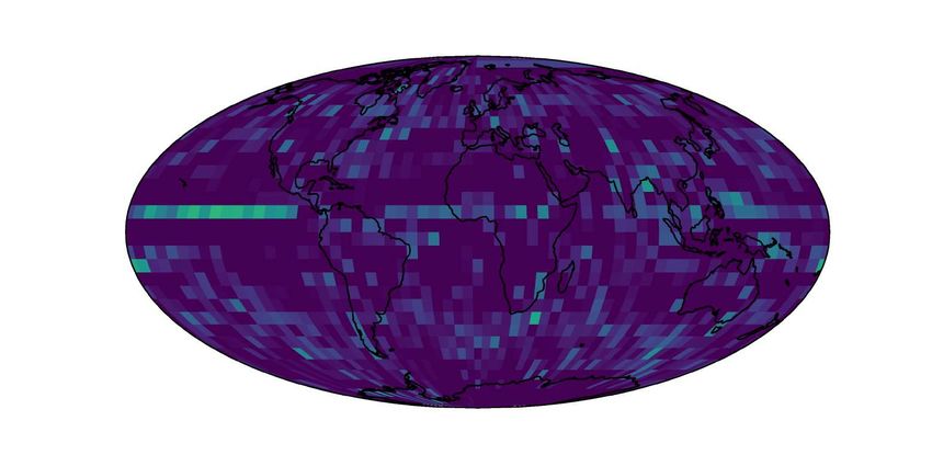
Table 3: Number of data samples loaded per second using PyRain versus a conventional NetCDF
framework. Typical configurations assumed and performed on a NVIDIA DGX1 server with 64
CPUs.
NetCDF PyRain Speedup
16 workers 40 2410 60.3×
64 workers 70 1930 27.6×
B Precipitation Events in ERA5 and IMERG
RainBench provides precipitation values in two forms: ERA5 precipitation and IMERG precipitation.
The ERA5 precipitation is accumulated precipitation over the last hour – in m – and is calculated as an
averaged quantity over a grid-box. IMERG precipitation has been aggregated into hourly accumulated
precipitation – in mm – and should be considered as a point estimate of the precipitation.
Figure 1 shows the distribution of precipitation for the years 2000-2017 with both ERA5 and IMERG.
Their different distributions indicate that the quality of global precipitation estimates, in particular
related to extreme precipitation events, varies with the choice of precipitation data. IMERG has
significantly larger rainfall tails than ERA5, and these tails rapidly vanish with decreasing dataset
resolution. The underestimation of extreme precipitation events in ERA5 is clearly visible.
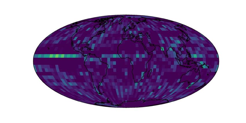
Figure 2 shows the pixel-wise precipitation class histograms derived from IMERG at native resolution
(0.1◦ ) with max-pooling as downscaling to preserve pixel-wise extremes.
100
ERA:tp 1.40625
10 2 ERA:tp 5.625
probability density
IMERG 0.25
10 4 IMERG 1.40625
IMERG 5.625
10 6
10 8
10 10
0 25 50 75 100 125 150 175 200
precipitation [mm/hour]
Figure 1: Precipitation histogram for the years 2000-2017 with both ERA5 and IMERG at different
resolutions. Vertical lines delineate convection rainfall types: slight (0 mm h−1 to 2 mm h−1 ), mod-
erate (2 mm h−1 to 10 mm h−1 ), heavy (10 mm h−1 to 50 mm h−1 ), and violent (over 50 mm h−1 )
[15].
C Data Preprocessing for Benchmark Tasks
To facilitate efficient experimentation, we convert all data from their original resolutions to lower
resolutions using bilinear interpolation. Throughout this paper, we consider data at 5.625◦ .
The chosen input features for benchmark tasks are as follows. From the ERA5 dataset, we select a
subset of variables as input to the forecast model based on our data analysis results; the inputs are
geopotential (z), temperature (t), humidity (q), cloud liquid water content (clwc), cloud ice water
content (ciwc), each sampled at 300 hPa, 500 hPa and 850 hPa geopotential heights; to these we
add the surface pressure and the 2-meter temperature (t2m), as well as static variables that describe
the location and surface of the Earth, i.e. latitude, longitude, land-sea mask, orography and soil
type. From the SimSat dataset, the inputs are cloud-brightness temperature (clbt) taken at three
wavelengths. We normalize each variable with its global mean and standard deviation.
Since the data from each source are available at different times, we use the subset of data available
from April 2016 train all models for the benchmark tasks, unless specified otherwise. We use data
from 2018 and 2019 as validation and test sets respectively. To make sure no overlap exists between
training and evaluation data, the first evaluated date is 6 January 2019 while the last training date is
31 December 2017.
8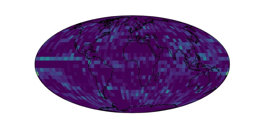
90 S                                                                                  100%       90 S                                                                                        5%
72 S                                                                                             72 S
54 S                                                                                             54 S
                                                                                      98%                                                                                                    3%
36 S                                                                                             36 S
18 S                                                                                             18 S
    0                                                                                 97%           0                                                                                        2%
18 N                                                                                             18 N
36 N                                                                                             36 N
                                                                                      96%                                                                                                    1%
54 N                                                                                             54 N
72 N                                                                                             72 N
90 N                                                                                  95%        90 N                                                                                        0%
   180 W 144 W 108 W   72 W   36 W     0   36 E    72 E    108 E    144 E    180 E                  180 W 144 W 108 W   72 W    36 W       0    36 E    72 E    108 E    144 E     180 E

                              (a) Slight Rain                                                                              (b) Moderate Rain

90 S                                                                                   1%        90 N                                                                                      0.10%
72 S                                                                                             72 N
54 S                                                                                             54 N
                                                                                       0%                                                                                                  0.07%
36 S                                                                                             36 N
18 S                                                                                             18 N
    0                                                                                  0%           0                                                                                      0.05%
18 N                                                                                             18 S
36 N                                                                                             36 S
                                                                                       0%                                                                                                  0.03%
54 N                                                                                             54 S
72 N                                                                                             72 S
90 N                                                                                   0%        90 S                                                                                      0.00%
   180 W 144 W 108 W   72 W    36 W    0    36 E    72 E    108 E    144 E    180 E                180 W 144 W 108 W    72 W    36 W   0       36 E    72 E    108 E    144 E    180 E

                              (c) Heavy Rain                                                                                   (d) Violent Rain
                                      Figure 2: Global distribution of rain events (% of total events).

D       Correlation Analysis

In Figure 3, we analyse the dependencies between all RainBench variables, we calculate pairwise
Spearman’s rank correlation indices over latitude band from −60 to 60◦ and date range from April
2016 to December 2019. In contrast to Pearson’s correlation coefficient, Spearman’s correlation
coefficient is significant if there is a, potentially non-linear, monotonic relationship between variables,
while Pearson’s considers only linear correlations. This allows to capture relationships between
variables such as between temperature and absolute latitude. Comparing correlations at altitude
pressure levels 300 hPa (about 10 km) and 850 hPa (1.5 km), we can see that they are almost
identical, save for a few exceptions: Specific humidity, q, and geopotential height, z, correlate
strongly at 300 hPa but not at 850 hPa, cloud ice water content, ciwc, generally correlates more
strongly at higher altitude (and cloud liquid water content, clwc, vice versa). A careful examination
of the underlying physical dependencies results in the realisation that all of these asymmetries stem
mostly from latitudinal correlations or effects related to cloud formation, e.g. ice and liquid form in
clouds at different temperatures/altitudes.
As we are particularly interested in variables that have predictive skill on precipitation, we note that
all SimSat spectral channels moderately anti-correlate with both ERA5 and IMERG precipitation
estimates. Interestingly, SimSat signals correlate much stronger with specific humidity and cloud
ice water content at higher altitude, which might be a consequence of spectral penetration depth.
ERA5 state variables that correlate most with either precipitation estimates are specific humidity and
temperature. Cloud ice water content correlates moderately strongly with precipitation estimates
at high altitude, but not at all at lower altitude (where ice water content tends to be much lower).
Interestingly, a number of time-varying ERA5 state variables correlate more strongly with IMERG
precipitation than ERA5 precipitation, as do SimSat signals. Conversely, a number of constant
variables, such as land-sea mask, orography and soil type are significantly anti-correlated with
ERA5 precipitation, but not at all correlated with IMERG. Overall, we find that all variables that
are significantly correlated or anti-correlated with both ERA5 tp and IMERG are also correlated or
anti-correlated with SimSat clbt:0-2, suggesting that precipitation prediction from simulated satellite
data alone may be feasible.

E       Model Implementation

We use Convolutional LSTMs [24] and structure our forecasting task based on MetNet’s configura-
tions [21]. An overview of our setup is shown in Figure 4.

                                                                                             9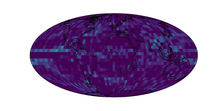
lon                                                1.00
                          lat
                        lsm                                                 0.75
                         oro
                          slt                                               0.50
                            z
                            t                                               0.25
                            q
                          sp                                                0.00
                      clwc
                      ciwc                                                    0.25
                       t2m
                     clbt:0                                                   0.50
                     clbt:1
                     clbt:2                                                   0.75
                           tp
                     imerg                                                    1.00
                                    oro

                                imerg
                                    lon
                                     lat
                                   lsm

                                     slt
                                       z
                                       t
                                       q
                                     sp
                                 clwc
                                 ciwc
                                  t2m
                                clbt:0
                                clbt:1
                                clbt:2
                                      tp
Figure 3: Spearman’s correlation of RainBench variables from April 2016 to December 2019 at a
spatial resolution of 5.625◦ in latitude band [−60◦ , 60◦ ] at pressure levels 300 hPa (about 10 km)
(upper triangle) and 850 hPa (1.5 km) (lower triangle). Legend: lon: longitude, lat: latitude, lsm:
land-sea mask, oro: orography (topographic relief of mountains), lst: soil type, z: geopotential
height, t: temperature, q: specific humidity, sp: surface pressure, clwc: cloud liquid water content,
ciwc: cloud ice water content, t2m: temperature at 2m, clbt:i: i−th SimSat channel, tp: ERA5 total
precipitation, imerg: IMERG precipitation. All correlations in this plot are statistically significant
(p < 0.05).

The network’s input is composed of a time series {xt }, where each xt is the set of standardized
features at time t, sampled in regular intervals ∆t from t = −T to t = 0; the output is a precipitation
forecast y at lead time t = τ ≤ τL . In addition to the aforementioned atmospheric features, static
features (e.g. latitude) along with three time-dependant features (hour, day, month) are repeated
per timestep. The input vector is then concatenated with a lead-time one-hot vector xτ . In our
experiments, we adopt T = 12 h, ∆t = 3 h and forecasts at 24-hour intervals up to τL = 120 h. We
note that we do not include precipitation as an input temporal feature.

                  Figure 4: Modelling setup for the benchmark forecasting tasks.

F    Forecast Visualization
Figure 5 shows example forecasts from one random input sequence across the different data settings
for predicting ERA5 precipitation. We observe that the forecasts can capture the general precipitation
distribution across the globe, but there is various degrees of blurriness in the outputs. As we shall
discuss later in the paper, considering probabilistic forecasts would be a promising solution to
blurriness, which might have arisen as the mean predicted outcome.

                                                  10
1-day 2-day 3-day 4-day 5-day
Truth
Simsat
ERA
Simsat
& ERA
Figure 5: ERA5 Precipitation forecasts on a random sample.
11You can also read