EXPLORING CROSS-CITY SEMANTIC SEGMENTATION OF ALS POINT CLOUDS
←
→
Page content transcription
If your browser does not render page correctly, please read the page content below
The International Archives of the Photogrammetry, Remote Sensing and Spatial Information Sciences, Volume XLIII-B2-2021
                                                XXIV ISPRS Congress (2021 edition)

   EXPLORING CROSS-CITY SEMANTIC SEGMENTATION OF ALS POINT CLOUDS

                                Yuxing Xie1,2* , Konrad Schindler3 , Jiaojiao Tian1 , Xiao Xiang Zhu1,2
          1
              Remote Sensing Technology Institute (IMF), German Aerospace Center (DLR), Oberpfaffenhofen, Germany
                                          {yuxing.xie, jiaojiao.tian, xiaoxiang.zhu}@dlr.de
                  2
                    Data Science in Earth Observation, Technical University of Munich (TUM), Munich, Germany
                                  3
                                    Photogrammetry and Remote Sensing, ETH Zürich, Switzerland
                                                          schindler@ethz.ch

                                                            Commission II

KEY WORDS: Point Clouds, Semantic Segmentation, Deep Learning, Transfer Learning, Domain Adaptation

ABSTRACT:

Deep learning models achieve excellent semantic segmentation results for airborne laser scanning (ALS) point clouds, if sufficient
training data are provided. Increasing amounts of annotated data are becoming publicly available thanks to contributors from all
over the world. However, models trained on a specific dataset typically exhibit poor performance on other datasets. I.e., there are
significant domain shifts, as data captured in different environments or by distinct sensors have different distributions. In this work,
we study this domain shift and potential strategies to mitigate it, using two popular ALS datasets: the ISPRS Vaihingen benchmark
from Germany and the LASDU benchmark from China. We compare different training strategies for cross-city ALS point cloud
semantic segmentation. In our experiments, we analyse three factors that may lead to domain shift and affect the learning: point
cloud density, LiDAR intensity, and the role of data augmentation. Moreover, we evaluate a well-known standard method of
domain adaptation, deep CORAL (Sun and Saenko, 2016). In our experiments, adapting the point cloud density and appropriate
data augmentation both help to reduce the domain gap and improve segmentation accuracy. On the contrary, intensity features can
bring an improvement within a dataset, but deteriorate the generalisation across datasets. Deep CORAL does not further improve
the accuracy over the simple adaptation of density and data augmentation, although it can mitigate the impact of improperly chosen
point density, intensity features, and further dataset biases like lack of diversity.

                     1. INTRODUCTION                                  strategies”), so as to employ machine learning when the source
                                                                      and target data follow different distributions. One natural ap-
Unordered point clouds in 3D space have become a standard             proach, often used for point clouds, is data augmentation to ar-
representation of spatial data, used across a wide range of ap-       tificially increase the diversity of the training data. Besides,
plications like digital mapping, building information model-          there are also more formal methods for so-called unsupervised
ling and transportation planning. An important task for many          domain adaptation, meaning statistically inspired strategies to
such applications is semantic segmentation, i.e., assigning a         adapt to a new target distributions for which only data, but
semantic class label to every point. As manual labelling is           no ground truth annotations, are available. Unsupervised do-
time-consuming and expensive, researchers have for a long             main adaptation has recently shown promise in 2D image pro-
time sought to automate that task. Thanks to deep neural net-         cessing (Wilson and Cook, 2020, Wang and Deng, 2018). Re-
works the accuracy of supervised semantic segmentation has            cently, some authors have also started to adopt it for 3D point
improved significantly in recent years. But deep learning re-         cloud interpretation (Wu et al., 2019, Luo et al., 2020, Jaritz et
lies on large quantities of annotated reference data. Labelling       al., 2020).
a sufficiently large and diverse training set for every location
and/or every sensor still presents a significant workload and is      Here, we investigate a number of elementary training strategies
not scalable. E.g., labelling 2km2 of ALS data from Dublin            for semantic segmentation of ALS point clouds across differ-
(Ireland) into 13 hierarchical multi-level classes took >2,500        ent cities. To that end, we work with two public ALS data-
person-hours (Zolanvari et al., 2019). More and more annot-           sets from Germany and China, and transfer models between
ated ALS data is available in public datasets and benchmarks,         them. In terms of semantic segmentation model, we construct
labelled according to various nomenclatures. If models trained        a residual U-net style convolution architecture and employ KP-
from such public data (source scenes) could be transferred to         Conv (Thomas et al., 2019) as the backbone, due to its proven
other target scenes, per-project annotation would become ob-          performance on ALS point clouds (Varney et al., 2020). In our
solete. However, in practice almost every project (including the      experiments, we analyse three factors that may affect general-
public datasets) is different in terms of source and target envir-    isation across cities: (i) the point density that is fed into the
onment. Machine learning models, in particular deep learning          network; (ii) the augmentation method employed to synthetic-
models, will tend to overfit to the source data and therefore de-     ally increase data diversity; and (iii) the influence of intensity
liver poor results when naively applied to new, previously un-        features (on top of pure point coordinates). Furthermore, in-
seen target data.                                                     spired by the success of unsupervised, statistical domain adapt-
                                                                      ation in image processing, we also evaluate the effectiveness
Many studies have explored strategies to mitigate domain              of a widely known method, deep CORAL (Sun and Saenko,
shift and overfitting (from here on simply termed “training           2016). We find that elementary measures, like setting a suitable

                                                 This contribution has been peer-reviewed.
                  https://doi.org/10.5194/isprs-archives-XLIII-B2-2021-247-2021 | © Author(s) 2021. CC BY 4.0 License.              247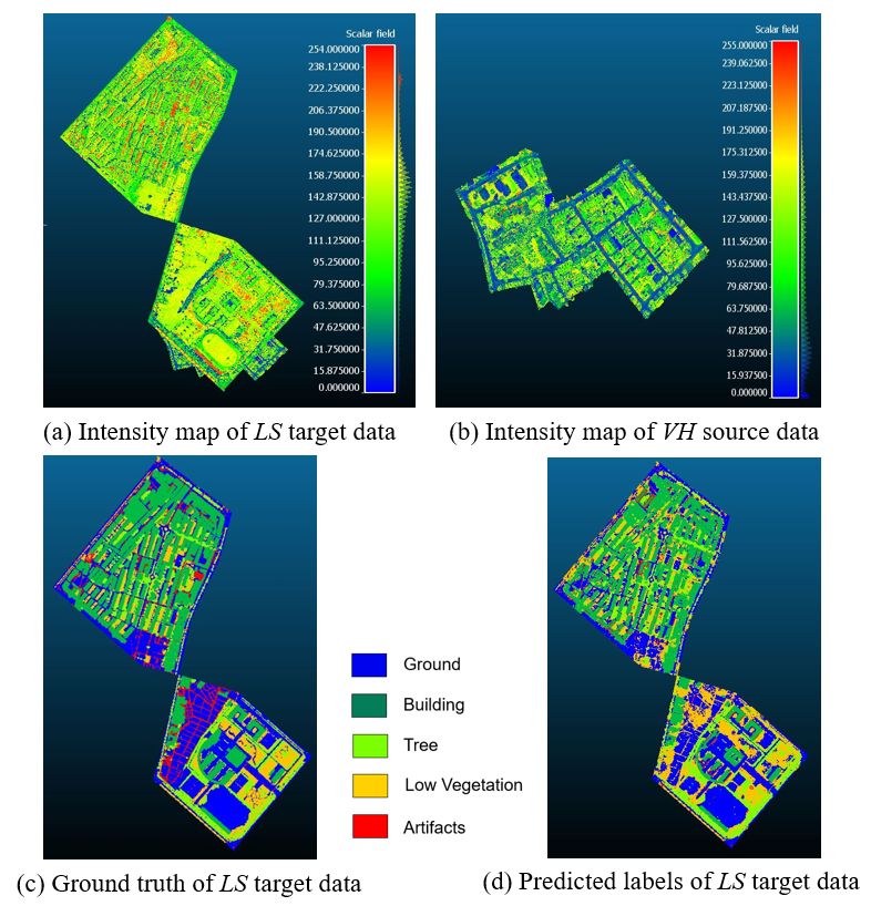
The International Archives of the Photogrammetry, Remote Sensing and Spatial Information Sciences, Volume XLIII-B2-2021
                                                 XXIV ISPRS Congress (2021 edition)

point density and augmentation, significantly benefit cross-city     Sörgel, 2019), and KPConv (Varney et al., 2020, Lin et al.,
generalisation, whereas deep CORAL does not further improve          2021) have also been adopted and have achieved good results
over them. On the contrary, intensity complicates generalisa-        on ALS data.
tion and might best be discarded when the generality of the
model is desirable.                                                  2.2   Training Strategies for Point Clouds

                    2. RELATED WORK                                  Data augmentation is an elementary training strategy for deep
                                                                     learning tasks (Shorten and Khoshgoftaar, 2019). Rotation,
This section reviews recent developments of point cloud se-          scaling, symmetry, random noise, and randomly removing
mantic segmentation, and associated training strategies aimed        points are common augmentation operations for point clouds
at improving generalisation.                                         (Chaton et al., 2020, Thomas et al., 2019). By synthetically in-
                                                                     creasing the diversity of patterns in the data, they can help to
2.1   Semantic Segmentation Techniques for Point Clouds              prevent overfitting when training data is limited. Recently, it
                                                                     has also been proposed to learn the data augmentation (Chen et
Point cloud semantic segmentation is a supervised classifica-        al., 2020, Li et al., 2020).
tion task. Shallow machine learning classifiers with manu-
ally designed features have been the traditional way to ad-          While, at first glance, deep learning continues to set the state
dress the problem, including for example support vector ma-          of the art on many public benchmarks, the situation in reality
chines (Zhang et al., 2013), random forests (Weinmann et al.,        is more complex. The excellent performance is achieved only
2015, Hackel et al., 2016), and Adaboost (Wang et al., 2014).        when trained on data from the same dataset, i.e., recorded in
The crucial step in this setting is feature extraction. For point    the same (or a very similar) environment with the same sensor
clouds, the most common features are basic geometric prop-           setup. Effectively, the semantic segmentation easily overfits to
erties, height-based features if the gravity direction is known,     the unique, specific conditions, so that domain shifts exist even
and features based on eigenvalues of the local point distribution    between seemingly similar datasets. From this extreme special-
(Weinmann et al., 2015, Hackel et al., 2016, Xu et al., 2019).       isation, due to the high capacity of deep networks, arises a need
Besides, graph-based neighborhood models such as conditional         for domain adaptation. This was first observed for 2D images
random fields have been utilised as a post-processing step to        (Wilson and Cook, 2020, Wang and Deng, 2018), but more re-
smooth the per-point labels (Landrieu et al., 2017).                 cently also explored for various 3D point cloud analysis tasks.
                                                                     In the setting of self-driving scenarios, (Langer et al., 2020, Wu
In recent years, deep learning has become the dominant ap-
                                                                     et al., 2019) first project LiDAR point clouds to images and then
proach for point cloud analysis. It requires no feature engin-
                                                                     apply imaged-based domain adaptation on them to aid semantic
eering and achieves better performance for many tasks includ-
                                                                     segmentation. For the important, point cloud-specific domain
ing semantic segmentation. Deep learning-based methods can
                                                                     shift of density differences, (Yi et al., 2020) formulate domain
be sorted into three main categories: image-based, voxel-based,
                                                                     adaptation as a complete-and-label problem. A voxel comple-
and point-based (Xie et al., 2020). Image-based methods pro-
                                                                     tion network is proposed to fill in gaps between the source and
ject point clouds to image-like 2D representations, then ap-
                                                                     target data, so they have similar density. xMUDA (Jaritz et al.,
ply 2D convolutions to them (Boulch et al., 2018, Yang et al.,
                                                                     2020) utilises cross-modal learning with images to address the
2017). Their main shortcoming is that they do not fully exploit
                                                                     domain shift between point clouds in road scenes. Mutual in-
the 3D geometry. Another solution is to discretise the point
                                                                     formation from cross-modal features is shown to improve se-
cloud to a regular, ordered voxel grid and then use regular 3D
                                                                     mantic segmentation. These works are aimed at point cloud
convolutions (Tchapmi et al., 2017). Voxel-based deep learn-
                                                                     semantic segmentation, but the domain adaptation strategies do
ing is time-consuming and memory-hungry, so most methods
                                                                     not directly operate on uni-modal point clouds. Towards dir-
now exploit the sparsity of the voxel space and employ sparse
                                                                     ect point cloud domain adaptation, (Luo et al., 2020) propose
convolutions (Choy et al., 2019, Graham et al., 2018) that only
                                                                     a framework that jointly aligns data and feature distributions
operate on non-empty voxels. Point-based methods include dif-
                                                                     of MLS point clouds, with a small network to refine the eleva-
ferent techniques that make it possible to operate directly on the
                                                                     tion of target data and an adversarial network to align the fea-
point cloud. They mainly differ by the way they define the ker-
                                                                     tures. (Peng et al., 2020) also address domain adaptation with
nels. The pioneering PointNet (Qi et al., 2017a) simply replaces
                                                                     adversarial learning and demonstrate their method for two sim-
convolution with a more general multi-layer perceptron (MLP).
                                                                     ilar ALS datasets (captured in the same region) and for an ALS
However, PointNet only learns global features, but not local
                                                                     dataset and a MLS dataset.
ones. To overcome this limitation, PointNet++ was proposed,
which captures local features via an image pyramid-like hier-
archical aggregation (Qi et al., 2017b). Several recent works
                                                                                         3. METHODOLOGY
instead design explicit convolution kernels for point clouds.
Among them, KPConv (Thomas et al., 2019) has demonstrated
high efficiency and good performance for point cloud semantic        We are not aware of any systematic comparison of different do-
segmentation, notably for large, mobile-mapping type outdoor         main adaptation strategies for point clouds. In this work, we set
scenarios.                                                           up a state-of-the-art semantic segmentation pipeline, with KP-
                                                                     Conv as the backbone, and compare several basic and practical
Also for ALS point clouds, deep learning is increasingly being       training strategies. We run experiments under different condi-
the method of choice. PointNet/PointNet++ has been widely            tions in terms of input point cloud density, data augmentation,
utilised as network backbone, since it appeared earlier (Yousef-     and the use of intensity features. Beyond these “hand-designed”
hussien et al., 2018, Lin et al., 2020, Huang et al., 2020). More    manipulations of the input data, we also test a classical, well-
recently, PointCNN (Arief et al., 2019), graph convolutions          established domain adaptation algorithm, deep CORAL (Sun
(Wen et al., 2021), spatially sparse convolution (Schmohl and        and Saenko, 2016).

                                                This contribution has been peer-reviewed.
                 https://doi.org/10.5194/isprs-archives-XLIII-B2-2021-247-2021 | © Author(s) 2021. CC BY 4.0 License.              248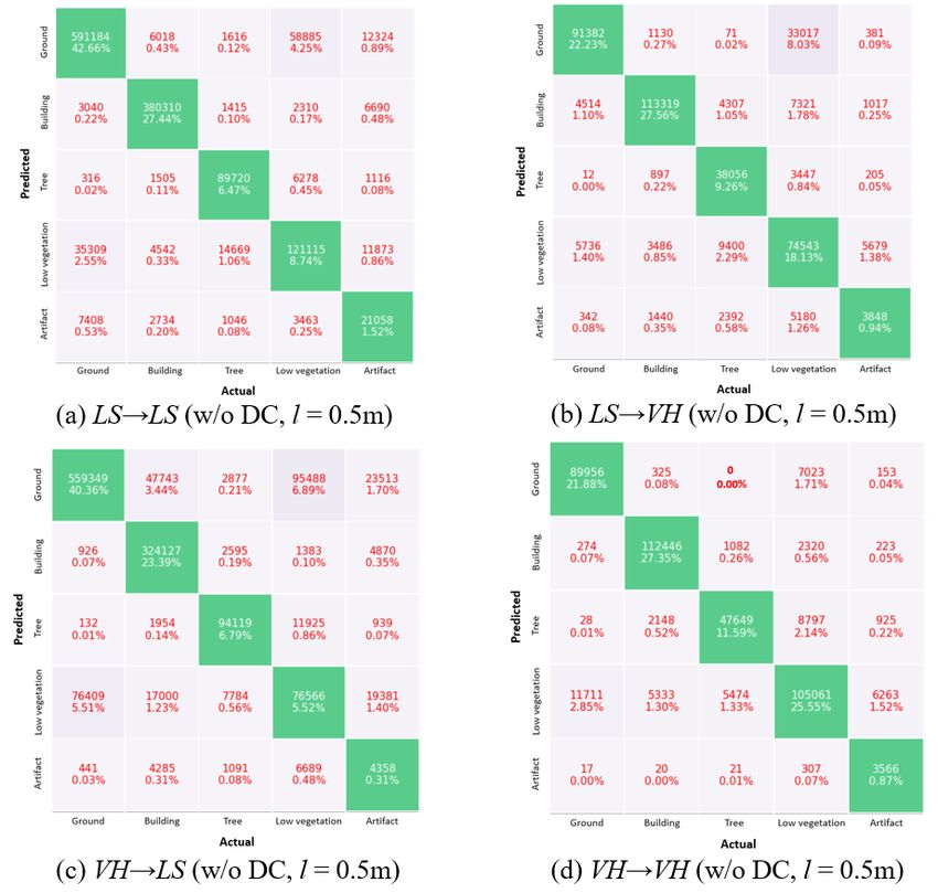
The International Archives of the Photogrammetry, Remote Sensing and Spatial Information Sciences, Volume XLIII-B2-2021
                                                 XXIV ISPRS Congress (2021 edition)

3.1   Semantic Segmentation by KPConv                                Deep CORAL imposes the correlation alignment as a soft con-
                                                                     straint, via the loss function. The CORAL loss is defined as the
KPConv (Thomas et al., 2019) is a direct point cloud convolu-        distance between the second-order statistics in the source and
tion operator, based on the idea to approximate the continuous       target feature matrices:
convolution operator in a local, spherical 3D neighbourhood.
Let pi and fi be points from a point cloud P ∈ RN ×3 and their                                     1
                                                                                      LCORAL =        kCS − CT k2 ,               (4)
corresponding features from F ∈ RN ×D . The point convolu-                                        4d2
tion at a point p ∈ RN ×3 is denoted as follows:
                                                                     with CS and CT the source and target feature covariance
                               X                                     matrices. During training, LCORAL is minimised with mini-
               (F ∗ g)(p) =            g(pi − p)fi ,          (1)    batches from the training set of the source domain and the target
                              pi ∈Np
                                                                     domain. The intuition behind deep CORAL is to “deform” the
                                                                     source and target feature distributions such that they match up
where g is the kernel function of KPConv. Np = {pi ∈                 to second-order statistics, assuming that the class-conditional
P | kpi − pk ≤ r} represent neighbour points of p within a           distributions will then match better, too.
fixed radius r ∈ R. In KPConv, g takes the those neighbours
centered on p as input to the convolution. The domain g is           Multiple CORAL loss functions over different activation layers
defined as a 3D sphere:                                              within the network can be combined, and added to the semantic
                                                                     segmentation loss Lseg , to obtain a joint loss function:
                  Br3 = {q ∈ R3 | kqk ≤ r} ,                  (2)
                                                                                                     t
                                                                                                     X         (i)
where qi = pi − p.                                                                Ltotal = Lseg +          λ(i) LCORAL ,          (5)
                                                                                                     i=1
KPConv provides two kernel versions, a rigid and a deformable
one. In the former, the kernel points are distributed in a fixed     where t is the number of layer-wise CORAL losses and λ(i) is
layout within the sphere, whereas the deformable one allows          the weight coefficient of the i-th CORAL loss.
for learned shifts of their positions. In practice, deformable KP-
Conv does not outperform the rigid version on scenes lacking         We train our KPConv-based residual U-net with standard cross-
diversity such as ALS point clouds (Thomas et al., 2019, Lin et      entropy loss for Lseg . Empirically, CORAL terms for lower
al., 2021) but requires more GPU memory and run time. Hence,         layers did not have much influence, so we only align the fea-
we use rigid KPConv in this work.                                    ture maps of the last activation layer with a single CORAL loss
                                                                     LCORAL . The network architecture is depicted in Figure 1. xSi
In our experiments we use the authors’ original PyTorch-based        and xT i represent input source and target samples, respectively.
implementation        (https://github.com/HuguesTHOMAS/              ySi is the set of input labels (given only for the input source
KPConv-PyTorch).        Our semantic segmentation embeds             data).
KPConv in a U-net architecture (Ronneberger et al., 2015),
following ResNet block design (He et al., 2016) in the encoder.
Each convolution layer in this network is followed by batch
normalization (BN) (Ioffe and Szegedy, 2015) and a Leaky
ReLU activation (Maas et al., 2013). Grid sampling is em-
ployed as the sub-sampling strategy to reduce the density and
increase the context along the layers. Hence, the data in each
layer are the center points of regularly spaced grid cells. The
convolution sphere radius ri for the i-th layer is adjusted by a
corresponding factor α, i.e.,

                           ri = αli ,                         (3)

where li and ri denote the grid size and convolution radius in
the i-th layer. Due to limited GPU RAM, the size of the input
sphere, and thus the size of the receptive field in the network,
are dependant on the grid spacing of first sub-sampling: wider
                                                                              Figure 1. Illustration of the network structure.
spacing causes stronger down-sampling (with potential loss of
information), but on the other hand allows for a larger receptive
field (with more context).                                                                4. EXPERIMENTS

3.2   Domain Adaptation by Deep CORAL                                4.1   Datasets

Correlation alignment is a popular, representative statistical al-   Two ALS point cloud benchmark datasets are adopted for the
gorithm for unsupervised domain adaptation. It tries to min-         evaluation: the ISPRS Vaihingen benchmark (Cramer, 2010,
imise the domain shift by aligning the second-order statistics       Rottensteiner et al., 2012) and LASDU (Ye et al., 2020). ISPRS
of source and target feature distributions, which can be done        Vaihingen was captured with a Leica ALS50 system from an
without any labels for the target domain. We adopt a deep ver-       average flying height of ≈500m in Vaihingen, Germany; while
sion of correlation alignment, named deep CORAL (Sun and             LASDU was captured with a Leica ALS70 system at an average
Saenko, 2016), which can be directly integrated into any neural      flying height of ≈1200m in a town of northwest China, which
network architecture.                                                is a part of the HiWATER (Heihe Watershed Allied Telemetry

                                                This contribution has been peer-reviewed.
                 https://doi.org/10.5194/isprs-archives-XLIII-B2-2021-247-2021 | © Author(s) 2021. CC BY 4.0 License.             249
The International Archives of the Photogrammetry, Remote Sensing and Spatial Information Sciences, Volume XLIII-B2-2021
XXIV ISPRS Congress (2021 edition)
Experimental Research) project (Li et al., 2013). The original (spherical) subsets of a large point cloud, we adopt the authors’
labels of LASDU (6 classes, including a rejection class “unclas- voting strategy during testing and average the estimated class
sified”) and ISPRS Vaihingen (9 classes) are different. How- probabilities of each point, obtained from at least 20 different
ever, for evaluation purposes the label sets of the two domains sphere samples. Training and testing were performed on a Ge-
should match. Hence, we map the 9 classes of ISPRS Vaihingen force RTX 2080 Ti GPU with 11GB RAM.
to the 6 classes of LASDU, following the classification rule of
LASDU. The “powerline” class of ISPRS Vaihingen is mapped Following the ISPRS Vaihingen benchmark, all results are eval-
to “others”, as no powerlines are labelled in LASDU. Points uated in terms of overall accuracy (OA) and F1 score.
with label “others” are used for training, but are ignored in the
quantitative evaluation. Table 1 shows the mapping between the 2T Pi
F 1i = , (6)
two label sets. 2T Pi + F Pi + F Ni
n
Classes of ISPRS Vaihingen Mapped classes Classes of LASDU X T Pi
Impervious surfaces Ground Ground OA = ( ), (7)
Roof, facade Building Building T Pi + T Ni + F Pi + F Ni
i=1
Tree Tree Tree
Low vegetation, bushes Low vegetation Low vegetation where i is the class index and TP refers to the number of true
Car, fence/hedge Artifact Artifact
Powerline Others (Ignored) Unclassified positives, FP the false positives, TN the true negatives, FN the
false negatives.
Table 1. Class mapping for ISPRS Vaihingen and LASDU point
cloud datasets. 4.3 Experiment I: Evaluation of Input Point Density
The ISPRS Vaihingen benchmark contains defined training and As explained in Section 3.1, an important hyper-parameter of
test portions. LASDU consists of four portions. It is recom- KPConv is the input point cloud density, i.e., in our setup
mended to use files 2 and 3 as the training data, and 1 and 4 defined via the grid size. A trade-off has to be found between
as the test set for semantic labelling (Ye et al., 2020). Table 2 input density and receptive field size. We test three settings for
shows the number of points in each class for both datasets. the grid spacing l: 0.25m, 0.5m and 0.8m. These correspond
to input context spheres of radius 13m, 25m and 40m, respect-
ISPRS Vaihingen LASDU ively. When l is bigger, the network can see a larger region, but
Mapped classes Training Test Training Test with sparser sampling and thus less geometric details and less
Ground 193,723 101,986 704,425 637,257 information on small objects. Data augmentation as described
Building 179,295 120,272 508,479 395,109 in Section 4.2 is used in all runs. LiDAR intensities are not
Tree 135,173 54,226 204,775 108,466
Low vegetation 228,455 123,508 210,495 192,051 used.
Artifact 16,684 11,130 66,738 53,061
Others (ignored) 546 600 33,206 12,659 Table 3 shows that the best generalisation results, for both
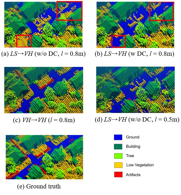
V H → LS and LS → V H , are achieved when l = 0.5m.
Table 2. Point distributions in ISPRS Vaihingen and LASDU Still, a clear domain shift exists. The OA of LS → V H (cross-
datasets. city) is 9 percent points (pp) lower than that of V H → V H
(within-city). Similarly, the OA of V H → LS is 10.5 pp lower
4.2 Experiment Setup and Evaluation Metrics than that of LS → LS . The F 1 scores are also lower across
all classes. Deep CORAL has a negative impact on the overall
Three experiments have been run. Each experiment includes six accuracy, due to more mistakes on the large ground and veget-
cases, obtained by using IPSRS Vaihingen (V H ) or LASDU ation classes. We note that in case of non-optimal sample dens-
(LS ) as source and target datasets and switching on (w DC) or ity l deep CORAL has a mild positive effect. In V H → LS
off (w/o DC) correlation alignment with deep CORAL. Writing (l = 0.25m), LS → V H (l = 0.25m) and LS → V H
A → B to denote training on dataset A and testing on B , the (l = 0.8m), the OA increases between 0.7 and 2.2 pp. It seems
six cases are: V H → V H , LS → V H (w/o DC), LS → V H that aligning the feature distributions somehow mitigates the
(w DC), LS → LS , V H → LS (w/o DC), and V H → LS domain difference for features derived from points sampled at
(w DC). In section 4.3, the influence of input grid size, i.e., sub-optimal density. An example for LS → V H is shown
point density is investigated. In section 4.4, the role of data in Figure 2. Note that at overly coarse sampling (0.8m) large
augmentation is assessed. Section 4.5 explores how intensity areas of ground points along roads are misclassified as low ve-
features affect accuracy and generalisation. getation, and deep CORAL corrects these errors. However, at
proper sampling density of l = 0.5m, the mistakes do not hap-
In all experiments, the batch size is set to 8 and α in equation pen in the first place, so there is no room for improvement.
3 is set to 2.5. Training with stochastic gradient descent (SGD)
is run for 60,000 iterations, at which point the loss function 4.4 Experiment II: Evaluation of Data Augmentation
has always converged. The initial learning rate is set to 0.01
and decays at a rate of 0.1 every 7,500 iterations when train- Deep neural networks require large training sets to avoid over-
ing on V H , respectively decays at the same rate every 12,500 fitting. Data augmentation is a technique to synthetically in-
iterations when training on the larger LS . Data augmentation, crease the sample size by manipulating existing samples in
including random rotation around the z -axis, random scaling, plausible ways. Table 4 presents results for the same settings
random symmetry about the x-axis, and Gaussian noise, is al- as above for grid spacing l = 0.5m, but without data augment-
ways applied except for the dedicated experiments without data ation, compared to Table 3. Again, LiDAR intensity values are
augmentation in Section 4.4. The scaling factor is randomized not used.
within [0.8, 1.2]. The standard deviation σ of Gaussian noise
is set to 5cm. When using correlation alignment the weight Comparing the numbers in Tables 4 and 3, we see that cross-
coefficient λ = 1.0. Since KPconv can only operate on limited city generalisation suffers if data augmentation is disabled. The
This contribution has been peer-reviewed.
https://doi.org/10.5194/isprs-archives-XLIII-B2-2021-247-2021 | © Author(s) 2021. CC BY 4.0 License. 250The International Archives of the Photogrammetry, Remote Sensing and Spatial Information Sciences, Volume XLIII-B2-2021
XXIV ISPRS Congress (2021 edition)
Input grid size Settings OA Ground Building Tree Low vegetation Artifact
VH →VH 0.8421 0.8427 0.9362 0.8272 0.7830 0.4306
LS → V H (w/o DC) 0.7433 0.7279 0.8683 0.7475 0.6765 0.0145
LS → V H (w DC) 0.7536 0.7862 0.8722 0.7986 0.5792 0.1002
l = 0.25m
LS → LS 0.8575 0.8892 0.9679 0.8670 0.5979 0.4025
V H → LS (w/o DC) 0.6809 0.7696 0.8099 0.8458 0.3677 0.0904
V H → LS (w DC) 0.6882 0.7616 0.8323 0.8627 0.3980 0.1172
VH →VH 0.8724 0.9021 0.9504 0.8376 0.8165 0.4735
LS → V H (w/o DC) 0.7812 0.8017 0.9038 0.7859 0.6705 0.3163
LS → V H (w DC) 0.7290 0.7348 0.9209 0.8244 0.4509 0.2469
l = 0.5m
LS → LS 0.8683 0.9044 0.9642 0.8652 0.6382 0.4744
V H → LS (w/o DC) 0.7638 0.8188 0.8892 0.8653 0.3935 0.1246
V H → LS (w DC) 0.7181 0.7576 0.9087 0.8585 0.4086 0.0844
VH →VH 0.8646 0.8902 0.9456 0.8322 0.8069 0.4730
LS → V H (w/o DC) 0.7422 0.7782 0.8508 0.7368 0.6145 0.3079
LS → V H (w DC) 0.7641 0.8026 0.8717 0.7548 0.8717 0.1581
l = 0.8m
LS → LS 0.8537 0.8860 0.9664 0.8665 0.5361 0.4306
V H → LS (w/o DC) 0.7409 0.8088 0.8696 0.8699 0.3981 0.1232
V H → LS (w DC) 0.6462 0.6348 0.9329 0.8573 0.3200 0.1294
Table 3. Results with different input grid spacing. Data augmentation was carried out but intensity features were not used.
OA decreased by 8 pp and 6 pp for LS → V H and V H → LS ,
respectively. Deep CORAL manages to mitigate that perform-
ance drop, improving OA by 2.8 pp and 4.2 pp, correspondingly.
However, its impact is again class-specific and the F 1 scores of
several classes are decreased significantly. In particular, in the
V H → LS test the F 1 scores for trees and buildings are lower
than before, and the score for artifacts even drops to 0.
4.5 Experiment III: Evaluation of Intensity
This experiment additionally assesses the role of intensity fea-
tures, which one might expect to also influence cross-city gen-
eralisation. In the original ISPRS Vaihingen and LASDU data-
sets, the LiDAR return intensities have already been scaled to
[0, 255], so we directly concatenate them with the 3D point co-
ordinates and feed the resulting 4D points to the network. Table
5 shows segmentation results with added intensities, at density
l = 0.5m, with data augmentation, compared to Table 3. Intens-
ities do improve the within-city results slightly for V H → V H
and more significantly for LS → LS , especially the separa-
tion of ground and low vegetation. This makes sense, as the
two classes are difficult to distinguish based only on geomet-
ric features – they both share low height and mostly horizontal,
planar layout. However, the performance for both LS → V H
and V H → LS drops significantly when using also intens-
ity. OA decreases by 5 pp for LS → V H , and even by 27
pp for V H → LS . As can be seen in Figure 3, the classifier
trained on V H misclassifies large regions of ground in LS as
low vegetation. One can see that the intensity distributions of
Figure 2. Example visualisation (experiment I). the two datasets differ significantly (Figure 3a and 3b), with al-
most all ground points in V H having low intensitiesThe International Archives of the Photogrammetry, Remote Sensing and Spatial Information Sciences, Volume XLIII-B2-2021
XXIV ISPRS Congress (2021 edition)
Settings OA Ground Building Tree Low vegetation Artifact
VH →VH 0.8329 0.8537 0.9275 0.8029 0.7665 0.4360
LS → V H (w/o DC) 0.7005 0.7885 0.7453 0.6361 0.6468 0.2725
LS → V H (w DC) 0.7281 0.7612 0.8800 0.7673 0.5564 0.2012
LS → LS 0.8608 0.8921 0.9692 0.8701 0.5750 0.4578
V H → LS (w/o DC) 0.7032 0.7749 0.8370 0.8371 0.3758 0.0886
V H → LS (w DC) 0.7455 0.8537 0.7626 0.6184 0.7499 0
Table 4. Results without data augmentation (l = 0.5m). Intensity features were not used.
Settings OA Ground Building Tree Low vegetation Artifact
VH →VH 0.8775 0.9153 0.9454 0.8291 0.8247 0.5595
LS → V H (w/o DC) 0.7302 0.7749 0.8549 0.7499 0.5363 0.2891
LS → V H (w DC) 0.7433 0.7571 0.9269 0.7934 0.5091 0.3874
LS → LS 0.8939 0.9225 0.9686 0.8736 0.7461 0.4517
V H → LS (w/o DC) 0.4897 0.2649 0.8748 0.8608 0.3241 0.0981
V H → LS (w DC) 0.5106 0.3634 0.8434 0.8217 0.3471 0
Table 5. Results with intensity (l = 0.5m). Data augmentation was carried out.
Figure 4. Confusion matrices.
4.6 Further Analysis
Confusion matrix. To analyse the class-wise effect of the
domain shift, we inspect confusion matrices of V H → LS ,
LS → LS , LS → V H , and V H → V H , for the best-
performing spacing l = 0.5m. In Figure 4 it can be seen that
an obvious issue in both the V H → LS and LS → V H res-
Figure 3. The inference result visualisation (experiment III). ults is indeed the confusion between low vegetation and ground,
due to their similar geometric characteristics. Within one data-
set intensity can to some degree compensate the mistake, but it
even extends the gap between the two point clouds. Arguably,
the two large classes associated with the ground are the main
challenge for domain adaptation between V H and LS .
Minority class. Minority classes, in our case especially arti-
facts, appear to be negatively affected by domain adaptation
This contribution has been peer-reviewed.
https://doi.org/10.5194/isprs-archives-XLIII-B2-2021-247-2021 | © Author(s) 2021. CC BY 4.0 License. 252The International Archives of the Photogrammetry, Remote Sensing and Spatial Information Sciences, Volume XLIII-B2-2021
XXIV ISPRS Congress (2021 edition)
with deep CORAL. In extreme cases, e.g., V H → LS (w Chaton, T., Chaulet, N., Horache, S., Landrieu, L., 2020. Torch-
DC) in Tables 4 and 5, the F 1 score even drops to 0. There points3d: A modular multi-task framework for reproducible
are multiple potential reasons for this behaviour. On the one deep learning on 3d point clouds. 2020 International Confer-
hand, the deep CORAL loss is calculated without taking into ence on 3D Vision (3DV), 190–199.
account the classes (which are unknown for the target distri-
bution). Rare classes will therefore have almost no influence Chen, Y., Hu, V. T., Gavves, E., Mensink, T., Mettes, P., Yang,
on the adaptation. And the resulting warping of the feature P., Snoek, C. G. M., 2020. Pointmixup: Augmentation for point
space, optimised to accommodate the dominant classes, can be clouds. European Conference on Computer Vision, Springer,
counter-productive. On the other hand, an aggravating factor 330–345.
might also be that the artifact class contains a too large vari- Choy, C., Gwak, J., Savarese, S., 2019. 4d spatio-temporal con-
ety of objects in LASDU, including walls, fences, light poles, vnets: Minkowski convolutional neural networks. Proceedings
vehicles, etc. The corresponding, wide and diffuse set of fea- of the IEEE Conference on Computer Vision and Pattern Re-
tures each valid only for few examples might lead to a com- cognition, 3075–3084.
plicated feature distribution not sufficiently characterised by the
second-order statistics. Cramer, M., 2010. The DGPF-test on digital airborne camera
evaluation overview and test design. PFG Photogrammetrie,
5. CONCLUSION Fernerkundung, Geoinformation, 73–82.
Graham, B., Engelcke, M., Van Der Maaten, L., 2018. 3d
We have empirically investigated cross-city learning of se-
semantic segmentation with submanifold sparse convolutional
mantic segmentation for ALS point clouds, using example data-
networks. Proceedings of the IEEE conference on computer vis-
sets from Germany and China. Three factors were considered
ion and pattern recognition, 9224–9232.
that all affect the results, and a representative, generic domain
adaptation strategy was evaluated. Our experiments indicate Hackel, T., Wegner, J. D., Schindler, K., 2016. Fast semantic
that data augmentation and proper choice of the input density segmentation of 3D point clouds with strongly varying dens-
play an important role and can significantly boost generalisa- ity. ISPRS annals of the photogrammetry, remote sensing and
tion performance. On the contrary, LiDAR intensities exhib- spatial information sciences, 3, 177–184.
ited stronger differences between datasets and might better be
avoided, as they negatively impact performance across datasets. He, K., Zhang, X., Ren, S., Sun, J., 2016. Deep residual learn-
As for unsupervised, statistical domain adaptation with deep ing for image recognition. Proceedings of the IEEE conference
CORAL, we found that when training conditions are not op- on computer vision and pattern recognition, 770–778.
timal (e.g., intensities present or point density not well chosen)
it brings a mild improvement, however it did not resolve the im- Huang, R., Xu, Y., Hong, D., Yao, W., Ghamisi, P., Stilla, U.,
portant problems and affected different classes rather unevenly. 2020. Deep point embedding for urban classification using ALS
Elementary design choices, like choosing the right input dens- point clouds: A new perspective from local to global. ISPRS
ity and using data augmentation, were much more important Journal of Photogrammetry and Remote Sensing, 163, 62–81.
to achieve acceptable generalisation. Surprisingly, when those Ioffe, S., Szegedy, C., 2015. Batch normalization: Accelerating
were set to support generalisation in the best possible way, cor- deep network training by reducing internal covariate shift. In-
relation alignment even deteriorated the result by reinforcing ternational conference on machine learning, PMLR, 448–456.
class-dependent biases.
Jaritz, M., Vu, T.-H., Charette, R. d., Wirbel, E., Pérez, P.,
In future work we would like to develop domain adaptation 2020. xmuda: Cross-modal unsupervised domain adaptation for
methods that are better suited for semantic segmentation of 3d semantic segmentation. Proceedings of the IEEE/CVF Con-
ALS point clouds. Another important step for future research ference on Computer Vision and Pattern Recognition, 12605–
will be to introduce datasets with larger class nomenclatures, to 12614.
analyse and tackle domain adaptation for application scenarios
with more fine-grained semantics. Landrieu, L., Raguet, H., Vallet, B., Mallet, C., Weinmann,
M., 2017. A structured regularization framework for spa-
ACKNOWLEDGEMENTS tially smoothing semantic labelings of 3D point clouds. ISPRS
Journal of Photogrammetry and Remote Sensing, 132, 102–
We thank the the German Society for Photogrammetry, Remote 118.
Sensing and Geoinformation (DGPF), Germany and the Insti-
Langer, F., Milioto, A., Haag, A., Behley, J., Stachniss, C.,
tute of Tibetan Plateau Research, Chinese Academy of Sci-
2020. Domain Transfer for Semantic Segmentation of LiDAR
ences, China, for providing the datasets. We thank Hugues
Data using Deep Neural Networks. Proc. of the IEEE/RSJ Intl.
Thomas for providing the open source code of KPConv.
Conf. on Intelligent Robots and System (IROS).
REFERENCES Li, R., Li, X., Heng, P.-A., Fu, C.-W., 2020. Pointaugment:
an auto-augmentation framework for point cloud classification.
Arief, H. A., Indahl, U. G., Strand, G.-H., Tveite, H., 2019. Ad- Proceedings of the IEEE/CVF Conference on Computer Vision
dressing overfitting on point cloud classification using Atrous and Pattern Recognition, 6378–6387.
XCRF. ISPRS Journal of Photogrammetry and Remote Sens-
ing, 155, 90–101. Li, X., Cheng, G., Liu, S., Xiao, Q., Ma, M., Jin, R., Che, T.,
Liu, Q., Wang, W., Qi, Y. et al., 2013. Heihe watershed allied
Boulch, A., Guerry, J., Le Saux, B., Audebert, N., 2018. telemetry experimental research (HiWATER): Scientific object-
SnapNet: 3D point cloud semantic labeling with 2D deep seg- ives and experimental design. Bulletin of the American Meteor-
mentation networks. Computers & Graphics, 71, 189–198. ological Society, 94(8), 1145–1160.
This contribution has been peer-reviewed.
https://doi.org/10.5194/isprs-archives-XLIII-B2-2021-247-2021 | © Author(s) 2021. CC BY 4.0 License. 253The International Archives of the Photogrammetry, Remote Sensing and Spatial Information Sciences, Volume XLIII-B2-2021
XXIV ISPRS Congress (2021 edition)
Lin, Y., Vosselman, G., Cao, Y., Yang, M. Y., 2020. Active and Varney, N., Asari, V. K., Graehling, Q., 2020. Dales: a large-
incremental learning for semantic ALS point cloud segmenta- scale aerial lidar data set for semantic segmentation. Proceed-
tion. ISPRS Journal of Photogrammetry and Remote Sensing, ings of the IEEE/CVF Conference on Computer Vision and Pat-
169, 73–92. tern Recognition Workshops, 186–187.
Lin, Y., Vosselman, G., Cao, Y., Yang, M. Y., 2021. Local and Wang, M., Deng, W., 2018. Deep visual domain adaptation: A
global encoder network for semantic segmentation of Airborne survey. Neurocomputing, 312, 135–153.
laser scanning point clouds. ISPRS Journal of Photogrammetry Wang, Z., Zhang, L., Fang, T., Mathiopoulos, P. T., Tong, X.,
and Remote Sensing, 176, 151–168. Qu, H., Xiao, Z., Li, F., Chen, D., 2014. A multiscale and hier-
archical feature extraction method for terrestrial laser scanning
Luo, H., Khoshelham, K., Fang, L., Chen, C., 2020. Unsuper- point cloud classification. IEEE Transactions on Geoscience
vised scene adaptation for semantic segmentation of urban mo- and Remote Sensing, 53(5), 2409–2425.
bile laser scanning point clouds. ISPRS Journal of Photogram-
metry and Remote Sensing, 169, 253–267. Weinmann, M., Jutzi, B., Hinz, S., Mallet, C., 2015. Semantic
point cloud interpretation based on optimal neighborhoods, rel-
Maas, A. L., Hannun, A. Y., Ng, A. Y., 2013. Rectifier nonlin- evant features and efficient classifiers. ISPRS Journal of Photo-
earities improve neural network acoustic models. Proceedings grammetry and Remote Sensing, 105, 286–304.
of International Conference on Machine Learning.
Wen, C., Li, X., Yao, X., Peng, L., Chi, T., 2021. Airborne
Peng, S., Xi, X., Wang, C., Xie, R., Wang, P., Tan, H., 2020. LiDAR point cloud classification with global-local graph atten-
Point-Based Multilevel Domain Adaptation for Point Cloud tion convolution neural network. ISPRS Journal of Photogram-
Segmentation. IEEE Geoscience and Remote Sensing Letters. metry and Remote Sensing, 173, 181–194.
Wilson, G., Cook, D. J., 2020. A survey of unsupervised deep
Qi, C. R., Su, H., Mo, K., Guibas, L. J., 2017a. Pointnet: Deep
domain adaptation. ACM Transactions on Intelligent Systems
learning on point sets for 3d classification and segmentation.
and Technology (TIST), 11(5), 1–46.
Proceedings of the IEEE conference on computer vision and
pattern recognition, 652–660. Wu, B., Zhou, X., Zhao, S., Yue, X., Keutzer, K., 2019.
Squeezesegv2: Improved model structure and unsupervised do-
Qi, C. R., Yi, L., Su, H., Guibas, L. J., 2017b. Pointnet++ deep main adaptation for road-object segmentation from a lidar point
hierarchical feature learning on point sets in a metric space. cloud. 2019 International Conference on Robotics and Automa-
Proceedings of the 31st International Conference on Neural In- tion (ICRA), IEEE, 4376–4382.
formation Processing Systems, 5105–5114.
Xie, Y., Tian, J., Zhu, X. X., 2020. Linking points with labels
Ronneberger, O., Fischer, P., Brox, T., 2015. U-net: Convo- in 3D: A review of point cloud semantic segmentation. IEEE
lutional networks for biomedical image segmentation. Interna- Geoscience and Remote Sensing Magazine, 8(4), 38–59.
tional Conference on Medical image computing and computer-
Xu, Y., Ye, Z., Yao, W., Huang, R., Tong, X., Hoegner, L.,
assisted intervention, Springer, 234–241.
Stilla, U., 2019. Classification of LiDAR point clouds using
Rottensteiner, F., Sohn, G., Jung, J., Gerke, M., Baillard, C., supervoxel-based detrended feature and perception-weighted
Benitez, S., Breitkopf, U., 2012. The ISPRS benchmark on graphical model. IEEE Journal of Selected Topics in Applied
urban object classification and 3D building reconstruction. IS- Earth Observations and Remote Sensing, 13, 72–88.
PRS Annals of the Photogrammetry, Remote Sensing and Spa- Yang, Z., Jiang, W., Xu, B., Zhu, Q., Jiang, S., Huang, W.,
tial Information Sciences I-3 (2012), Nr. 1, 1(1), 293–298. 2017. A convolutional neural network-based 3D semantic la-
beling method for ALS point clouds. Remote Sensing, 9(9),
Schmohl, S., Sörgel, U., 2019. Submanifold Sparse Convo- 936.
lutional Networks for Semantic Segmentation of Large-Scale
ALS Point Clouds. ISPRS Annals of Photogrammetry, Remote Ye, Z., Xu, Y., Huang, R., Tong, X., Li, X., Liu, X., Luan, K.,
Sensing and Spatial Information Sciences, 42, 77–84. Hoegner, L., Stilla, U., 2020. LASDU: A Large-Scale Aerial
LiDAR Dataset for Semantic Labeling in Dense Urban Areas.
Shorten, C., Khoshgoftaar, T. M., 2019. A survey on image data ISPRS International Journal of Geo-Information, 9(7), 450.
augmentation for deep learning. Journal of Big Data, 6(1), 1–
48. Yi, L., Gong, B., Funkhouser, T., 2020. Complete & label:
A domain adaptation approach to semantic segmentation of
Sun, B., Saenko, K., 2016. Deep coral: Correlation alignment LiDAR point clouds. arXiv preprint arXiv:2007.08488.
for deep domain adaptation. European conference on computer Yousefhussien, M., Kelbe, D. J., Ientilucci, E. J., Salvaggio, C.,
vision, Springer, 443–450. 2018. A multi-scale fully convolutional network for semantic
labeling of 3D point clouds. ISPRS journal of photogrammetry
Tchapmi, L., Choy, C., Armeni, I., Gwak, J., Savarese, S., 2017. and remote sensing, 143, 191–204.
Segcloud: Semantic segmentation of 3d point clouds. 2017 in-
ternational conference on 3D vision (3DV), IEEE, 537–547. Zhang, J., Lin, X., Ning, X., 2013. SVM-based classification of
segmented airborne LiDAR point clouds in urban areas. Remote
Thomas, H., Qi, C. R., Deschaud, J.-E., Marcotegui, B., Sensing, 5(8), 3749–3775.
Goulette, F., Guibas, L. J., 2019. Kpconv: Flexible and de-
formable convolution for point clouds. Proceedings of the Zolanvari, S. M. I., Ruano, S., Rana, A., Cummins, A., da Silva,
IEEE/CVF International Conference on Computer Vision, R. E., Rahbar, M., Smolic, A., 2019. Dublincity: Annotated
6411–6420. lidar point cloud and its applications. BMVC.
This contribution has been peer-reviewed.
https://doi.org/10.5194/isprs-archives-XLIII-B2-2021-247-2021 | © Author(s) 2021. CC BY 4.0 License. 254You can also read