Measurement report: regional trends of stratospheric ozone evaluated using the MErged GRIdded Dataset of Ozone Profiles (MEGRIDOP)
←
→
Page content transcription
If your browser does not render page correctly, please read the page content below
Atmos. Chem. Phys., 21, 6707–6720, 2021
https://doi.org/10.5194/acp-21-6707-2021
© Author(s) 2021. This work is distributed under
the Creative Commons Attribution 4.0 License.

Measurement report: regional trends of stratospheric ozone
evaluated using the MErged GRIdded Dataset
of Ozone Profiles (MEGRIDOP)
Viktoria F. Sofieva1 , Monika Szelag
                                   ˛ 1 , Johanna Tamminen1 , Erkki Kyrölä1 , Doug Degenstein2 , Chris Roth2 ,
Daniel Zawada , Alexei Rozanov , Carlo Arosio3 , John P. Burrows3 , Mark Weber3 , Alexandra Laeng4 ,
                2                 3

Gabriele P. Stiller4 , Thomas von Clarmann4 , Lucien Froidevaux5 , Nathaniel Livesey5 , Michel van Roozendael6 , and
Christian Retscher7
1 Finnish  Meteorological Institute, Helsinki, Finland
2 Institute of Space and Atmospheric Studies, University of Saskatchewan, Saskatoon, Canada
3 Institute of Environmental Physics, University of Bremen, Bremen, Germany
4 Karlsruhe Institute of Technology, Institute of Meteorology and Climate Research, Karlsruhe, Germany
5 Jet Propulsion Laboratory, California Institute of Technology, Pasadena, California, USA
6 Royal Belgian Institute for Space Aeronomy (BIRA-IASB), Brussels, Belgium
7 ESA/ESRIN, Frascati, Italy

Correspondence: Viktoria F. Sofieva (viktoria.sofieva@fmi.fi)

Received: 26 October 2020 – Discussion started: 11 November 2020
Revised: 10 March 2021 – Accepted: 15 March 2021 – Published: 4 May 2021

Abstract. In this paper, we present the MErged GRIdded              The MEGRIDOP dataset has also been used to evalu-
Dataset of Ozone Profiles (MEGRIDOP) in the stratosphere         ate regional vertically resolved ozone trends in the strato-
with a resolved longitudinal structure, which is derived from    sphere, including the polar regions. It is found that strato-
data from six limb and occultation satellite instruments:        spheric ozone trends exhibit longitudinal structures at North-
GOMOS, SCIAMACHY and MIPAS on Envisat, OSIRIS                    ern Hemisphere middle and high latitudes, with enhanced
on Odin, OMPS on Suomi-NPP, and MLS on Aura. The                 trends over Scandinavia and the Atlantic region. This agrees
merged dataset was generated as a contribution to the Euro-      well with previous analyses and might be due to changes in
pean Space Agency Climate Change Initiative Ozone project        dynamical processes related to the Brewer–Dobson circula-
(Ozone_cci). The period of this merged time series of ozone      tion.
profiles is from late 2001 until the end of 2018.
   The monthly mean gridded ozone profile dataset is pro-
vided in the altitude range from 10 to 50 km in bins of 10◦      1   Introduction
latitude × 20◦ longitude. The merging is performed using
deseasonalized anomalies. The created MEGRIDOP dataset           Nowadays, the importance of protecting the ozone layer and
can be used for analyses that probe our understanding of         monitoring its recovery from the effect of ozone depleting
stratospheric chemistry and dynamics. To illustrate some         substances is well recognized (e.g., Petropavlovskikh et al.,
possible applications, we created a climatology of ozone pro-    2019; WMO, 2014, 2018). Past analyses have demonstrated
files with resolved longitudinal structure. We found zonal       that ozone is recovering in the upper stratosphere (e.g., Aro-
asymmetry in the climatological ozone profiles at middle and     sio et al., 2019; Bourassa et al., 2014; Kyrölä et al., 2013;
high latitudes associated with the polar vortex. At northern     Petropavlovskikh et al., 2019; Sofieva et al., 2017b; Stein-
high latitudes, the amplitude of the seasonal cycle also has a   brecht et al., 2017; WMO, 2018). The ozone recovery in
longitudinal dependence.                                         the lower stratosphere has not yet been observed, and lower
                                                                 stratospheric ozone trends are the subject of recent contro-

Published by Copernicus Publications on behalf of the European Geosciences Union.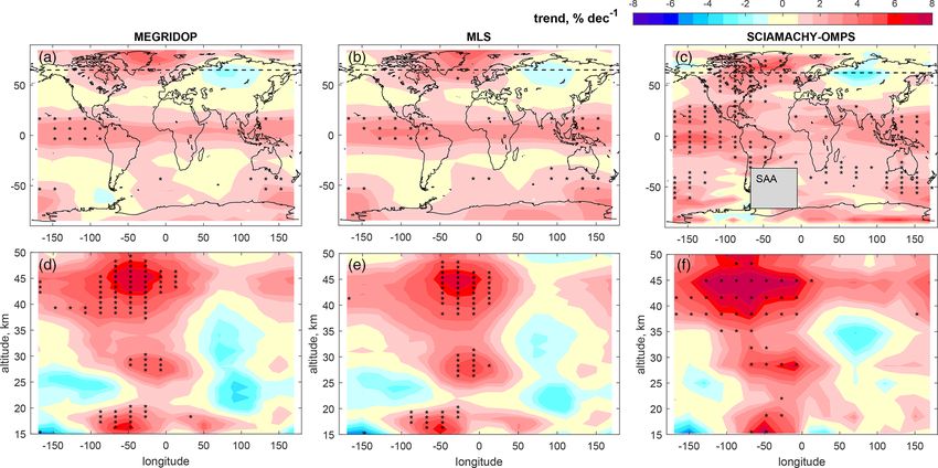
6708                                                               V. F. Sofieva et al.: Regional trends of stratospheric ozone

versial discussions (Ball et al., 2018, 2019; Chipperfield et      sity ozone profiles; therefore this representation (number
al., 2018).                                                        density on an altitude grid) is used for the merged dataset.
   In the majority of studies of ozone profile trends using        For MIPAS, the retrievals are performed in a volume mix-
satellite observations made in limb-viewing geometry, anal-        ing ratio vs. altitude grid. The conversion to number den-
yses are performed on zonal mean data. This representation         sity profiles is performed using temperature profiles re-
allows ozone trends to be estimated globally. At the same          trieved by MIPAS and the pressure profiles provided with
time, such representation provides a sufficiently large amount     the MIPAS ozone data; the latter are constructed from
of experimental data in spatiotemporal bins (usually 10◦ lati-     altitude and temperature using one (z, p, T ) data point
tude and 1 month) to enable robust estimation of trends. This      from the ERA-Interim reanalysis (https://www.ecmwf.int/
is especially important for the period before 2001 when long       en/forecasts/datasets/reanalysis-datasets/era-interim, last ac-
data records are available only from solar occultation instru-     cess: 22 April 2021; Dee et al., 2011).
ments having relatively sparse data coverage.                         For MLS, retrievals are performed in a mixing ratio on
   A recent study by Arosio et al. (2019) using the merged         a pressure grid. Similarly to the conversion procedure of
SCIAMACHY-OMPS dataset has shown that ozone trends                 MIPAS data, we performed the conversion to number den-
for the period from 2003–2018 have a significant dependence        sity using the retrieved MLS temperatures, but for altitude–
on longitude. Also, total ozone column trends (WMO, 2018           pressure conversion, we used the ERA-Interim reanalysis
and references therein) have a pronounced zonal structure.         data. Such a conversion might introduce some uncertainty
   This paper is focused on a new longitudinally resolved          in the MLS data. For studies of long-term changes, this un-
merged dataset of ozone profiles in the stratosphere based on      certainty is associated with a potentially imperfect represen-
several limb and occultation instruments. This new merged          tation of temperature trends in ERA-Interim, which might
dataset is a contribution to the European Space Agency Cli-        influence ozone trends. However, since current stratospheric
mate Change Initiative ozone project (Ozone_cci). It can be        temperature trends (after 2000) are small (Maycock et al.,
used in different applications, including the evaluation of re-    2018; Steiner et al., 2020), this uncertainty is expected to be
gional ozone trends in the stratosphere.                           small. The MLS ozone profiles data record is stable (Hubert
   The paper is organized as follows. In Sect. 2, we briefly       et al., 2016); therefore, including MLS data into the merged
discuss the satellite data used for creating the merged dataset.   dataset is advantageous, especially for the merging method
Section 3 is dedicated to the methodological aspects of            applied in our work (see also below).
data merging. Examples of ozone distributions are shown in            For all the instruments, we use the ozone profiles
Sect. 4. Section 5 is dedicated to regional trend analysis. A      from the updated HARMonized dataset of Ozone profiles
discussion and summary (Sect. 6) conclude the paper.               (HARMOZ_ALT) developed in the ESA Ozone_cci project
                                                                   (Sofieva et al., 2013), https://climate.esa.int/en/projects/
                                                                   ozone/ (last access: 22 April 2021). HARMOZ consists of
2   Data                                                           the original retrieved ozone profiles from each instrument,
                                                                   which are screened for invalid data by the instrument experts
The MEGRIDOP dataset is a merged and gridded dataset               and are presented on a vertical grid (altitude-gridded profiles
generated using ozone profiles retrieved from several limb         are used in our paper) and in a common netCDF4 format.
and occultation instruments, viz. MIPAS (Michelson In-             Detailed information about the original datasets can be found
terferometer for Passive Atmospheric Sounding), SCIA-              in Sofieva et al. (2013), and references to the corresponding
MACHY (SCanning Imaging Spectrometer for Atmospheric               publications are also collected in Table 1 of our paper.
CHartographY) and GOMOS (Global Ozone Monitoring by
occultation of Stars), all on Envisat, OSIRIS (Optical Spec-
trograph and InfraRed Imaging System) on Odin, OMPS-               3     Merging method
LP (Ozone Mapping and Profiles Suite – Limb Profiler) on
Suomi-NPP, and MLS (Microwave Limb Sounder) on Aura.               The method used for creating the MEGRIDOP dataset is sim-
   These instruments provide high-quality ozone profiles           ilar to that used for the creation of the merged SAGE-CCI-
with a good vertical resolution of 2–4 km and a relatively         OMPS dataset (Sofieva et al., 2017b). Below we describe and
dense spatiotemporal coverage (100–3500 ozone profiles per         illustrate the merging process.
day with fairly uniform sampling in longitude). The im-
portant information about the datasets is collected in Ta-         3.1    Gridded monthly means from individual
ble 1. More information about the datasets from the indi-                 instruments
vidual satellite instruments is found in Petropavlovskikh et
al. (2019), Sofieva et al. (2017b) and references therein.         First, gridded ozone profile data ρi (z, b, t) in each 10◦ × 20◦
   For all instruments except MLS, the original ozone pro-         latitude–longitude bin b and at altitude z were created for
file retrievals are performed on an altitude grid. GOMOS,          each individual dataset i and each month t. The mean number
OSIRIS, SCIAMACHY and OMPS-LP provide number den-                  density profile in each spatiotemporal bin is ρi (z, b, t). For

Atmos. Chem. Phys., 21, 6707–6720, 2021                                              https://doi.org/10.5194/acp-21-6707-2021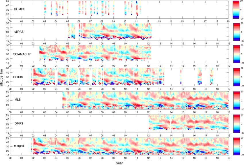
V. F. Sofieva et al.: Regional trends of stratospheric ozone                                                                              6709

Table 1. General information about the datasets.

          Instrument/        Level 2 processor,         Years            Vertical              Local time of           Number of
          satellite          references                                  range/retrieval       level 2 data            profiles per day
                                                                         coordinate
          MIPAS/             KIT/IAA                    2005–2012        6–70 km,              10:00 and               ∼ 1000
          Envisat            V7R_O3_240                                  altitude              22:00
                             (von Clarmann et al.,
                             2003, 2009)
          SCIAMACHY/         UBr v3.5                   2002–2012        8–65 km,              10:00                   ∼ 1300
          Envisat            (Jia et al., 2015)                          altitude
          GOMOS/             ALGOM2s v1                 2002–2011        10–105 km,            22:00                   ∼ 110
          Envisat            (Kyrölä et al., 2010;                       altitude
                             Sofieva et al., 2017a)
          OSIRIS/            USask v5.10                2001–present     10–59 km,             06:00 and               ∼ 250
          Odin               (Bourassa et al., 2018;                     altitude              18:00
                             Degenstein et al., 2009)
          OMLS-LP/           USask 2D v 1.1.0           2012–present     6–59 km,              13:30                   ∼ 1600
          SUOMI-NPP          (Zawada et al., 2018)                       altitude
          MLS/               NASA v4.2                  2004–present     261–0.02 hPa          01:30 and               ∼ 3000
          Aura               (Livesey et al., 2013)                      (∼ 8–75 km),          13:30
                                                                         pressure

each instrument, we required more than 10 measurements in              measure Htime is used for detection of spatial bins with high
each spatiotemporal bin. The uncertainty of the averaged data          inhomogeneity of data (see below).
σi (z, b, t) is approximated by the standard error of the mean
(see discussion in Toohey and von Clarmann, 2013 on pos-               3.2   Seasonal cycle and deseasonalized anomalies
sible influence of correlations caused by orbital sampling on
the standard error of the mean).                                       For each instrument i, latitude–longitude bin b and altitude
   The non-uniformity of the sampling pattern can be char-             level z, deseasonalized anomalies are computed as:
acterized by the inhomogeneity measure, which is defined as
                                                                                        ρi (z, b, t) − ρm,i (z, b)
the linear combination of two classical inhomogeneity mea-             1i (z, b, t) =                              ,                       (1)
sures, asymmetry A and entropy E: H = 12 (A + (1 − E))                                          ρm,i (z, b)
(Sofieva et al., 2014). The unitless inhomogeneity measure
                                                                       where ρi (z, b, t) is the monthly mean in this spatial bin and
H ranges from 0 to 1 (the more homogeneous, the smaller
                                                                       ρm,i (z, b) is the climatological mean value for the month m.
H is). For our application, we considered the inhomogeneity
                                                                       In other words, from each January we removed the mean Jan-
in time (Htime ) as the main contribution to sampling uncer-
                                                                       uary value, from each February the mean February value, and
tainty.
                                                                       so on.
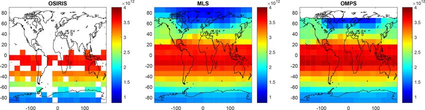
   Examples of gridded datasets at 30 km altitude for indi-
                                                                          In our computations, we removed values for spatial bins
vidual satellite instruments are shown in Figs. 1 and 2. All
                                                                       with less than 10 profiles and inhomogeneity Htime larger
instruments show a similar morphology, although biases be-
                                                                       than 0.9. For all instruments except for OMPS, the sea-
tween individual datasets exist. The coverage is instrument-
                                                                       sonal cycle is estimated using the years from 2005–2011.
specific and to some extent time-dependent; the most com-
                                                                       For OMPS, the seasonal cycle is evaluated using data from
plete coverage is achieved by MIPAS and MLS. The spatial
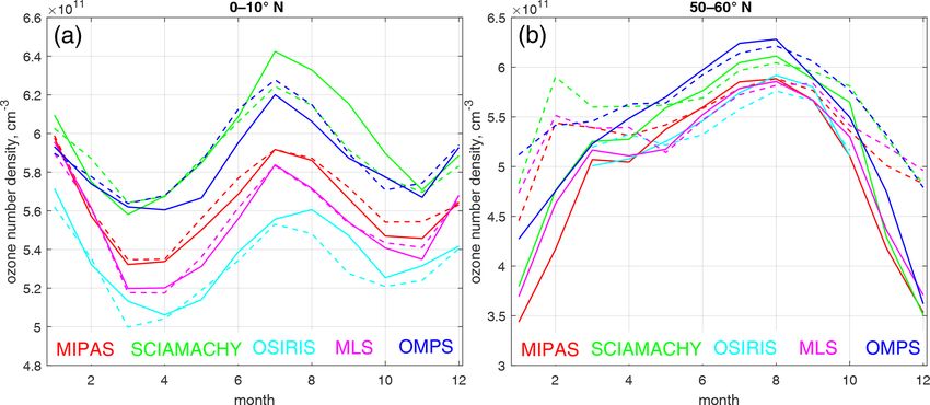
                                                                       2012–2018. Figure 3 illustrates the seasonal cycle at 40 km
bins are covered rather uniformly by the data. Examples of
                                                                       for all instruments except GOMOS, as the GOMOS data do
the inhomogeneity measure Htime are presented in Fig. S1
                                                                       not cover all months for the considered spatial bins. Although
in the Supplement. Htime is very close to zero for the instru-
                                                                       biases are visible, the overall behavior of the seasonal cycle
ments with dense sampling (MIPAS, SCIAMACHY, MLS,
                                                                       is similar for the different datasets. In the tropics (left panel),
OMPS). For OSIRIS and GOMOS, H is usually below 0.1
                                                                       small differences in seasonal cycle between two longitude
(good homogeneity of the data) with a few exceptions for
                                                                       regions, 0–20 and 120–140◦ E, are observed, while at mid-
some months and locations. In this work, the inhomogeneity
                                                                       latitudes, all satellite instruments show consistently different
                                                                       seasonal cycles in these two longitude regions.

https://doi.org/10.5194/acp-21-6707-2021                                                   Atmos. Chem. Phys., 21, 6707–6720, 2021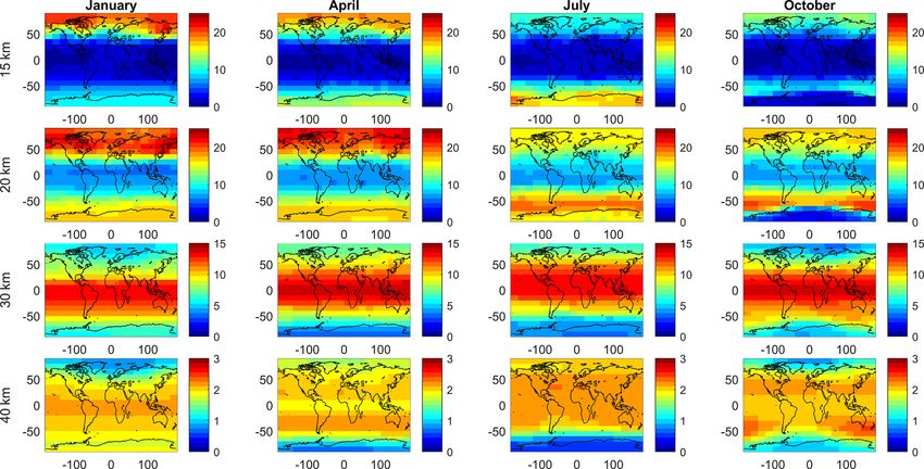
6710                                                                  V. F. Sofieva et al.: Regional trends of stratospheric ozone

Figure 1. Examples of gridded monthly mean ozone number density (cm−3 ) at 30 km for individual satellite instruments in January 2008.

Figure 2. Examples of gridded monthly mean ozone number density (cm−3 ) at 30 km for individual satellite instruments in January 2018.

   For two instruments – MIPAS and MLS – which measure                3.3   Merging the data
during day and night and thus provide data at all latitudes in
all seasons, we compared the relative amplitude of the sea-           The merging method used for creating MEGRIDOP is sim-
sonal cycle max(ρ m )−min(ρm )
                 mean(ρm )     at several altitude levels (Fig. 4).   ilar to that used in creating the merged SAGE-CCI-OMPS
As seen from Fig. 4, longitudinal structures in the relative          dataset (Sofieva et al., 2017b). The deseasonalized anomalies
amplitude of the seasonal cycle are observed to be largest            of all instruments except OMPS are aligned, as the seasonal
in the northern middle and high latitudes, particularly in the        cycle was estimated using the same period. First, we offset
middle and upper stratosphere.                                        the OMPS deseasonalized anomalies to the median of the de-
   The merging of individual datasets was performed on de-            seasonalized anomalies from all other instruments. These ad-
seasonalized anomalies. The main advantage of using desea-            ditive offsets are computed using the data from years 2012–
sonalized anomalies is that various biases between the indi-          2018, and the offsetting procedure is illustrated in Fig. 5. In
vidual datasets – e.g., instrumental-specific, or those due to        this figure, we selected a spatial bin where the effect of the
the difference in local time – are automatically removed. The         offsetting is clearly visible. In many other bins, the offsets
deseasonalization also removes spatial sampling biases if the         are small or negligible. As observed in Fig. 5 (and also be-
sampling patterns do not change over time. Details of the ap-         low in Fig. 6), the deseasonalized anomalies from individual
plied merging method are presented in the next section.               datasets are in good agreement.
                                                                         After offsetting OMPS, the merged ozone profiles in each
                                                                      spatiotemporal bin and at each altitude level is obtained from

Atmos. Chem. Phys., 21, 6707–6720, 2021                                                 https://doi.org/10.5194/acp-21-6707-2021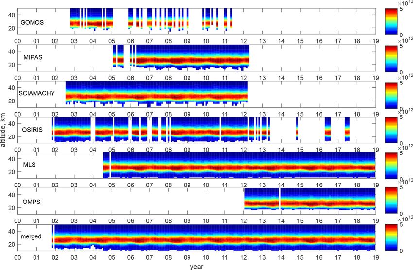
V. F. Sofieva et al.: Regional trends of stratospheric ozone                                                                           6711

Figure 3. Examples of seasonal cycles in the tropics (a) and NH upper stratosphere (b) at 40 km. Solid lines: longitudes 0–20◦ E; dashed
lines: longitudes 120–140◦ E. In the tropics, a semi-annual cycle is observed.

Figure 4. Relative amplitude of seasonal cycle at 25 km (a, d), 35 km (b, e) and 45 km (c, f) for MIPAS (a, b, c) and MLS (d, e, f).

the median of the deseasonalized anomalies corresponding                 CCI-OMPS dataset (Sofieva et al., 2017b). For each instru-
to individual instruments:                                               ment, the uncertainty of the deseasonalized anomalies, σ1i ,
                                                                         is estimated via Gaussian error propagation; it is given by
1merged (z, b, t) = median(1i (z, b, t)).                       (2)
                                                                                    v
                                                                                    u 2    2
                                                                                          σm,i
The advantage of using the median estimate is that the                              uσ
merged anomaly follows the majority of the data and it is                σ1i   = 1i t i2 + 2 ,                                          (3)
                                                                                      ρi  ρm,i
not very sensitive to exclusion or addition of an individual
data record in cases where there are several (and consistent)
anomaly datasets available. The sensitivity of the dataset and           where σi is the uncertainty of the gridded ozone profiles (see
the evaluated trends to the number of instruments was studied            Sect. 3.1) and σm,i is the uncertainty of the seasonal cycle
in detail for the SAGE-CCI-OMPS dataset, which is created                ρm,i , which can be estimated via propagation of random un-
with the same merging algorithm (Sofieva et al., 2017b), and             certainties to the mean value:
this is also valid for MEGRIDOP.                                                      Nm
   The uncertainties of the merged deseasonalized anomalies               2        1 X
                                                                         σm,i =           σ 2 (z, b, tj ),                              (4)
are computed similarly to those used for the merged SAGE-                         Nm2 j =1 i

https://doi.org/10.5194/acp-21-6707-2021                                                    Atmos. Chem. Phys., 21, 6707–6720, 2021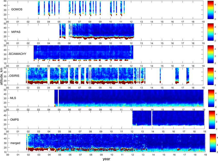
6712                                                                  V. F. Sofieva et al.: Regional trends of stratospheric ozone

Figure 5. Illustration of offsetting the OMPS deseasonalized anomalies. The data are shown for altitude 35 km and the 0–10◦ N, 0–20◦ E
bin.

where Nm is the number of monthly mean values in a given              4   The merged dataset and selected examples
month m available from all years.
   Analogously to Sofieva et al. (2017b), the uncertainties of        The merged deseasonalized anomalies can be directly used
the merged deseasonalized anomalies are estimated as                  for evaluation of ozone trends in the stratosphere. The eval-
                                                                      uation of regional ozone trends is discussed in Sect. 5 of our
σ1,merged =                                                           paper. We also created a version of MEGRIDOP in number
                r
                    1 XN          1 XN                 2
                                                          !           density through restoration of the seasonal cycle. This was
                             2
min σ1,jmed ,              σ
                       j =1 1,j
                                + 2  j =1
                                          1j − 1merged      ,   (5)   achieved in a manner similar to that applied in creating the
                    N            N
                                                                      merged SAGE-CCI-OMPS dataset (Sofieva et al., 2017b).
where σ1,imed is the anomaly uncertainty of the instrument            The best estimates of the amplitude and morphology of the
corresponding to the median value. In cases where there are           seasonal cycle are provided by MIPAS and MLS, as these
an even number of measurements, the mean of two neigh-                two instruments provide global coverage in all seasons. The
bors to the median is used. Analogously to uncertainty esti-          ozone profiles from OSIRIS and MLS have the smallest bi-
mates in the merged SAGE-CCI-OMPS dataset (Sofieva et                 ases with respect to ozone soundings (Hubert et al., 2016).
al., 2017b), the uncertainties given by Eq. (5) can be inter-         For the seasonal cycle of the merged dataset, we computed
preted as follows. If individual anomalies are significantly          the mean of MIPAS and MLS seasonal cycles and offset it
different, the uncertainty of the merged anomaly is the uncer-        to the mean of OSIRIS and MLS values (this offset does not
tainty corresponding to the median value. In cases where sev-         depend on season). Using this procedure, the seasonal cycle
eral instruments report a similar anomaly (intersecting error         in the merged dataset has absolute values, which have the
bars), this provides more confidence in this anomaly value,           smallest biases with respect to the ground-based instruments
and the resulting uncertainty of the merged anomaly is ap-            and a realistic amplitude. An example of a number density
proximated by the second term in Eq. (5).                             MEGRIDOP dataset is shown in Fig. 8.
   The deseasonalized anomalies from individual datasets are             The merged dataset allows us to provide a gridded clima-
usually very close to each other so that several values can be        tology of ozone profiles, i.e., the collection of ozone profiles
typically found within the uncertainty interval of the merged         categorized by calendar month, latitude, longitude and alti-
anomaly 1merged ± σ1,merged . This is similar to the approach         tude. Figure 9 shows these climatological ozone values for 4
taken with the SAGE_CCI-OMPS dataset (Sofieva et al.,                 months and at four altitude levels. The polar projections of
2017b, Fig. S8).                                                      these distributions are presented in the Supplement (Figs. S2
   Examples of deseasonalized anomalies and their estimated           and S3). As observed in these figures, there is zonal asym-
uncertainties are displayed in Figs. 6 and 7, respectively.           metry associated with the polar vortex in both hemispheres.
   The average estimated uncertainty of the merged ozone is           In other locations, the ozone distributions are rather uniform
usually less than 2 % before 2012 and below 1 % after 2012.           in longitude.
In the upper troposphere and the lower stratosphere (UTLS),
uncertainties are larger than in the stratosphere; they are typ-
ically in the range of 2 %–12 % before 2012 and 2 %–6 %
after 2012.

Atmos. Chem. Phys., 21, 6707–6720, 2021                                                 https://doi.org/10.5194/acp-21-6707-2021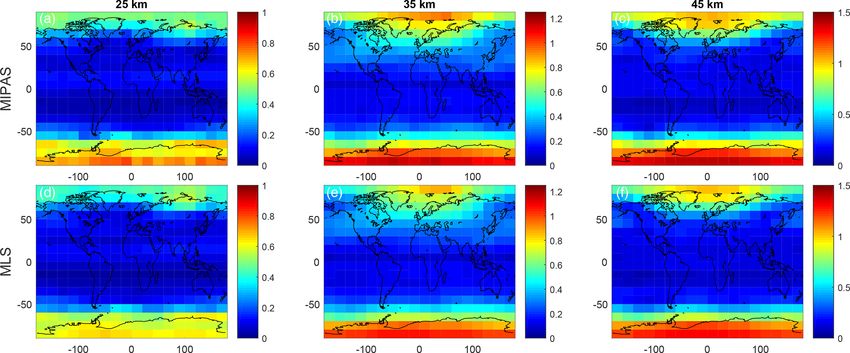
V. F. Sofieva et al.: Regional trends of stratospheric ozone                                                                     6713

Figure 6. An example of deseasonalized anomalies (in %) for individual instruments and the merged dataset in the spatial bin 0–10◦ N,
0–20◦ E.

5   Evaluation of regional ozone trends                              linear function (which describes bulk changes). However,
                                                                     real changes in the atmosphere can be non-linear (Laine et
For evaluation of the regional ozone trends, we exploited the        al., 2014): if variations are analyzed on a shorter timescale,
standard approach of multiple linear regression and applied          they can be different from long-term trends (e.g., Arosio et
it to the deseasonalized anomalies:                                  al., 2019; Chipperfield et al., 2018; Galytska et al., 2019;
1merged (t) = at + b + q1 QBO30 (t) + q2 QBO50 (t)                   Strahan et al., 2020). We selected the years after 2003 in or-
                                                                     der to avoid the influence of a major sudden stratospheric
           + sF10.7 (t) + dENSO(t),                         (6)      warming in September 2002 on ozone trends at Southern
where we model the trend with a simple linear term,                  Hemisphere middle and high latitudes (see also the discus-
QBO30 (t) and QBO50 (t) are the equatorial winds at                  sion below).
30 and 50 hPa, respectively (http://www.cpc.ncep.noaa.gov/              Ozone trends (expressed in percent per decade) estimated
data/indices/, last access: 22 April 2021), F10.7 (t) is the         at several altitude levels for the years from 2003–2018 are
monthly average solar 10.7 cm radio flux (https://www.ngdc.          shown in Fig. 10. Figure 11 displays the trends at these al-
noaa.gov/stp/solar/flux.html, last access: 25 April 2021) and        titudes in absolute units, DU km−1 decade−1 ). In Figs. 10
ENSO(t) is the 2 month lagged ENSO proxy (https://psl.               and 11, black stars indicate the statistically significant trends,
noaa.gov/enso/mei/, last access: 23 April 2021). The eval-           i.e., trends different from zero at a 95 % or greater con-
uation of trends has been performed for each latitude–               fidence level. The morphology of ozone trends presented
longitude bin and for each altitude level separately. Auto-          in absolute and in relative units look similar. As shown
correlations are removed using the Cochrane–Orcutt trans-            in Figs. 10 and 11, statistically significant trends are ob-
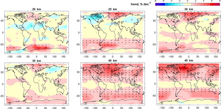
formation (Cochrane and Orcutt, 1949).                               served in the upper stratosphere. A longitudinal structure is
   In our analysis, we consider long-term trends over the            clearly visible in the NH mid-latitude trends above 40 km: the
years covered by MEGRIDOP and approximate them by a                  trends are significantly larger over Scandinavia and the north-

https://doi.org/10.5194/acp-21-6707-2021                                              Atmos. Chem. Phys., 21, 6707–6720, 2021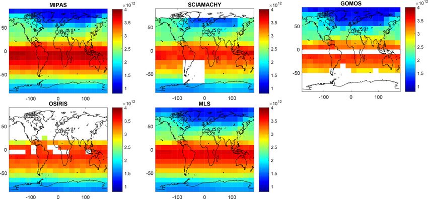
6714                                                                  V. F. Sofieva et al.: Regional trends of stratospheric ozone

Figure 7. An example of uncertainties in deseasonalized anomalies (in %) for individual instruments and the merged dataset in the spatial
bin 0–10◦ N, 0–20◦ E.

ern Atlantic Ocean (5 %–6 % decade−1 ) than over Siberia                  There are several analyses showing that the residual cir-
(∼ 1 % decade−1 ). The same feature was also observed by               culation has a pronounced longitudinal two-core structure
Arosio et al. (2019). Enhanced ozone trends over the mid-              at Northern Hemisphere high and middle latitudes (e.g.,
latitude Atlantic sector are seen in both absolute and relative        Demirhan Bari et al., 2013; Kozubek et al., 2015). Kozubek
units, and also at lower altitudes (but the ozone trends are not       et al. (2015) also performed a trend analysis and showed a
statistically significant below 40 km).                                weakening of the two-core structure, which possibly affects
   We also compared the trends in late 2004–2018, the com-             the ozone distribution in the region. Arosio et al. (2019) sug-
mon measurement period, using MEGRIDOP, only MLS                       gested that this longitudinal structure in the NH mid-latitude
data and the merged SCIAMACHY-OMPS dataset by Aro-                     ozone trends is due to changes in dynamical processes related
sio et al. (2019). We found that the spatial distributions of          to the 3D structure of the Brewer–Dobson circulation. How-
ozone trends are similar for the considered datasets (Fig. 12,         ever, the origin of the longitudinal structure of ozone trends
top). The MEGRIDOP and pure MLS ozone trends in 2004–                  requires more detailed investigations in the future, including
2018 are similar (as expected, MLS data are used in MEGRI-             simulations with chemistry-transport models.
DOP). SCIAMACHY-OMPS trends are somewhat larger,                          Statistically significant (at 95 % confidence level) posi-
which might be related to the OMPS drift (Kramarova et al.,            tive trends (1 %–2 % decade−1 ) are also observed at SH mid-
2018), but within error limits, and the morphology of ozone            latitudes (∼ 40–50◦ S) at 25 km. This is in agreement with
trends is similar. Specifically interesting is a two-core struc-       other studies of zonally averaged ozone trends (e.g., Aro-
ture of ozone trends in the NH polar region, and this is seen          sio et al., 2019; Petropavlovskikh et al., 2019; Sofieva et
nearly at all altitude levels (Fig. 12, bottom) for all datasets.      al., 2017b). In our analysis, there is a zonal asymmetry with

Atmos. Chem. Phys., 21, 6707–6720, 2021                                                  https://doi.org/10.5194/acp-21-6707-2021
V. F. Sofieva et al.: Regional trends of stratospheric ozone                                                                          6715

Figure 8. An example of number density ozone profiles (in cm−3 ) for individual instruments and the merged dataset in the spatial bin
0–10◦ N, 0–20◦ E.

Figure 9. Climatological ozone distributions (in DU km−1 ) for January, April, July and October for selected altitude levels (15, 20, 30 and
40 km).

https://doi.org/10.5194/acp-21-6707-2021                                                   Atmos. Chem. Phys., 21, 6707–6720, 2021
6716                                                                     V. F. Sofieva et al.: Regional trends of stratospheric ozone

Figure 10. Ozone trends (% decade−1 ) in 2003–2018 for several altitudes. Statistically significant trends are indicated by stars.

Figure 11. Same as Fig. 10, but for trends in DU km−1 decade−1 .

larger trends in the sector 50◦ W–10◦ E. At altitudes of 20–              trends at ∼ 35 km to the selection of the period for evalu-
25 km, the trend patterns are different in the Northern and               ation of ozone trends has been reported in several papers
Southern Hemispheres.                                                     (e.g., Laine et al., 2014; Arosio et al., 2019; Galytska et al.,
   Comparisons of MEGRIDOP ozone trends at 35 km in                       2019). As a hypothesis, this might be related to a decadal-
Figs. 10 and 12 show larger positive ozone trends in the trop-            scale ozone oscillation resulting from changes in Brewer–
ics in the period from 2004–2018 compared to the period                   Dobson Circulation.
from 2003–2018. A pronounced sensitivity of tropical ozone

Atmos. Chem. Phys., 21, 6707–6720, 2021                                                      https://doi.org/10.5194/acp-21-6707-2021
V. F. Sofieva et al.: Regional trends of stratospheric ozone                                                                           6717

Figure 12. (a, b, c) Ozone trends in late 2004–2018 (% decade−1 ) at 35 km and (d, e, f) longitude–altitude cross section of the ozone trends
at ∼ 65◦ N (the latitude is indicated by a dashed line on the top panels). Ozone trends are estimated using the MEGRIDOP (a, d), MLS (b,
e) and SCIAMACHY-OMPS datasets (c, f). For the SCIAMACHY-OMPS dataset, ozone trends in the Southern Atlantic Anomaly (SAA)
region are not shown because SCIAMACHY data are flagged in this region.

   In previous studies (e.g., Petropavlovskikh et al., 2019;             (Solomon et al., 2016; Szelag  ˛ et al., 2020; Galytska et al.,
Steinbrecht et al., 2017; WMO, 2018), ozone trends have                  2019) can be explored in future work. In addition, the relation
been evaluated at latitudes 60◦ S–60◦ N, i.e., excluding po-             of winter–spring trends with respect to the position of the
lar regions. In this study, we have made an attempt to also              polar vortex would be an interesting subject in future studies.
evaluate ozone trends in polar regions. The ozone trends in                 The satellite data quality typically degrades in the UTLS
polar projections are shown in the Supplement.                           compared to higher levels in the stratosphere. Our merg-
   We found statistically significant positive trends in the NH          ing principle seems to be particularly optimal for the UTLS
polar middle stratosphere (25–30 km). In the SH polar re-                datasets, as it automatically removes biases, which can be
gions, the estimated ozone trends are mostly positive, but               significant in this altitude region. The very large natural
they are not statistically significant. We found that the es-            ozone variability results in MEGRIDOP trend estimates be-
timated trends in the SH polar regions are sensitive to the              low 20 km being not statistically significant in most loca-
inclusion of 2002 data into the trend analysis. Quite excep-             tions.
tional (larger) ozone values in 2002 due to a SH major sudden
stratospheric warming result in negative, although not statis-
tically significant, ozone trends in the SH polar stratosphere,          6   Summary
as expected since 2002 is at the beginning of the time pe-
riod. If data from 2002 are excluded from the analysis, the              In this paper, we presented the merged gridded dataset of
estimated trends over Antarctica are not sensitive to the se-            ozone profiles (MEGRIDOP), which combines ozone data
lection of the starting point for the trend analysis. This can           from six limb-viewing satellite instruments. The merged
be observed, for example, by comparison of ozone trends at               gridded ozone profiles are the monthly means in 10◦ × 20◦
35 km in Fig. 10 (trends for 2003–2018) and Fig. 12 (trends              latitude–longitude bins, and they cover altitudes from 10 to
for late 2004 to 2018).                                                  50 km. This dataset covers the years from 2001–2018 and
   Since natural variability is high in polar regions and the            will be extended regularly in the future.
observational period is relatively short, it is quite expected              The merging was performed using aligned deseasonalized
that a simple multiple regression will lead to trend estimates           anomalies: the merged dataset represents the median of the
that are not statistically significant. Other methods for trend          deseasonalized anomalies from the individual instruments.
analysis in polar regions, such as considering seasonal trends           The merged deseasonalized anomalies can be used directly
                                                                         for evaluation of ozone trends. For other applications, the

https://doi.org/10.5194/acp-21-6707-2021                                                   Atmos. Chem. Phys., 21, 6707–6720, 2021
6718 V. F. Sofieva et al.: Regional trends of stratospheric ozone
MEGRIDOP is also available in the form of ozone number ments, methods, and science applications (AMT/ACP inter-journal
density profiles. SI)”.
The MEGRIDOP dataset can be used in different analyses.
As an illustration of one of the possible applications, a clima-
tology of ozone profiles with resolved longitudinal structure Acknowledgements. The work is performed in the framework of
has been created. We found zonal asymmetry in the climato- the ESA Ozone_cci+ project. The GOMOS ALGOM2s dataset was
logical ozone profiles at middle and high latitudes associated created in the framework of ESA ALGOM project. The KIT team
would like to thank the European Space Agency (ESA) for giving
with the polar vortex. At northern high latitudes, the ampli-
access to MIPAS level-1 data. The SCIAMACHY ozone retrieval
tude of the seasonal cycle also has a longitudinal dependence.
was funded in parts by the ESA, the German Academic Exchange
We evaluated regional ozone trends over the years from Service (DAAD), the German Aerospace Agency (DLR), and the
2001–2018 using a multiple linear regression method. Over- University and State of Bremen. The dataset was calculated with
all, the estimated trends agree well with the trends derived resources provided by the North-German Supercomputing Alliance
from zonal mean ozone profiles. We found a zonal asymme- (HLRN). The study is also a contribution to the German Ministry of
try in the upper stratospheric ozone trends at middle and high Education and Research (BMBF) Synopsis Project. The FMI team
latitudes in the Northern Hemisphere: the trends are larger thanks the Academy of Finland. The authors thank the Canadian
over Scandinavia than over Siberia. This feature agrees well Space Agency. Work at the Jet Propulsion Laboratory, California
with previous analyses and might be due to changes in dy- Institute of Technology, was performed under contract with the Na-
namical processes related to the Brewer–Dobson circulation. tional Aeronautics and Space Administration (NASA).
We also estimated regional and vertically resolved ozone
trends in the polar regions. As far as we know, this is the first
Financial support. This research has been supported by
such analysis using limb satellite measurements. We found
the European Space Agency (Ozone_cci+ project, con-
statistically significant positive trends in the NH polar mid-
tract 4000126562/19/I-NB), the EU Copernicus Climate
dle stratosphere (25–30 km). In the SH polar regions, the es- Change Service for Atmospheric Composition ECVs (con-
timated ozone trends are mostly positive, but they are not tract C3S_312b_Lot2_DLR_2018SC1), the German Academic
statistically significant. Exchange Service (DAAD), the German Aerospace Agency
The MEGRIDOP dataset can be used in different analyses. (DLR), the University and State of Bremen, the German Federal
In particular, it can be used for intercomparison of climate Ministry for Economic Affairs and Energy (project SEREMISA),
data records from ground-based and other satellite measure- the Academy of Finland (the Centre of Excellence of Inverse
ments and chemistry-transport models in the future. Modelling and Imaging (decision 336798)), the Canadian Space
Agency and the National Aeronautics and Space Administration
(Contract 80NM0018D0004).
Data availability. The dataset is available through open access
at https://climate.esa.int/en/projects/ozone/data/ and at ftp://cci_
web@ftp-ae.oma.be/esacci (ESA Climate Office, last access: 25 Review statement. This paper was edited by Jens-Uwe Grooß and
April 2021). reviewed by two anonymous referees.
Supplement. The supplement related to this article is available on-
line at: https://doi.org/10.5194/acp-21-6707-2021-supplement. References
Arosio, C., Rozanov, A., Malinina, E., Weber, M., and Burrows, J.
Author contributions. VFS designed the study, performed analyses P.: Merging of ozone profiles from SCIAMACHY, OMPS and
and wrote the major part of the manuscript. MS participated in trend SAGE II observations to study stratospheric ozone changes, At-
analyses. MS, JT, EK, DD, CR, DZ, AR, CA, JPB, MW, AL, GPS, mos. Meas. Tech., 12, 2423–2444, https://doi.org/10.5194/amt-
TvC, LF, NL, MvR and CR provided the data and contributed to 12-2423-2019, 2019.
analyses and manuscript writing. Ball, W. T., Alsing, J., Mortlock, D. J., Staehelin, J., Haigh, J.
D., Peter, T., Tummon, F., Stübi, R., Stenke, A., Anderson, J.,
Bourassa, A., Davis, S. M., Degenstein, D., Frith, S., Froidevaux,
Competing interests. Gabriele P. Stiller, Thomas von Clarmann and L., Roth, C., Sofieva, V., Wang, R., Wild, J., Yu, P., Ziemke, J.
Michel van Roozendael are editors of ACP, but have not been in- R., and Rozanov, E. V.: Evidence for a continuous decline in
volved in the evaluation of this paper. lower stratospheric ozone offsetting ozone layer recovery, At-
mos. Chem. Phys., 18, 1379–1394, https://doi.org/10.5194/acp-
18-1379-2018, 2018.
Ball, W. T., Alsing, J., Staehelin, J., Davis, S. M., Froidevaux, L.,
Special issue statement. This article is part of the special issue
and Peter, T.: Stratospheric ozone trends for 1985–2018: sensi-
“New developments in atmospheric limb measurements: instru-
tivity to recent large variability, Atmos. Chem. Phys., 19, 12731–
12748, https://doi.org/10.5194/acp-19-12731-2019, 2019.
Atmos. Chem. Phys., 21, 6707–6720, 2021 https://doi.org/10.5194/acp-21-6707-2021V. F. Sofieva et al.: Regional trends of stratospheric ozone 6719 Bourassa, A. E., Degenstein, D. A., Randel, W. J., Zawodny, J. ozone profile data records, Atmos. Meas. Tech., 9, 2497–2534, M., Kyrölä, E., McLinden, C. A., Sioris, C. E., and Roth, C. Z.: https://doi.org/10.5194/amt-9-2497-2016, 2016. Trends in stratospheric ozone derived from merged SAGE II and Jia, J., Rozanov, A., Ladstätter-Weißenmayer, A., and Burrows, J. Odin-OSIRIS satellite observations, Atmos. Chem. Phys., 14, P.: Global validation of SCIAMACHY limb ozone data (versions 6983–6994, https://doi.org/10.5194/acp-14-6983-2014, 2014. 2.9 and 3.0, IUP Bremen) using ozonesonde measurements, At- Bourassa, A. E., Roth, C. Z., Zawada, D. J., Rieger, L. A., McLin- mos. Meas. Tech., 8, 3369–3383, https://doi.org/10.5194/amt-8- den, C. A., and Degenstein, D. A.: Drift-corrected Odin-OSIRIS 3369-2015, 2015. ozone product: algorithm and updated stratospheric ozone trends, Kozubek, M., Krizan, P., and Lastovicka, J.: Northern Hemisphere Atmos. Meas. Tech., 11, 489–498, https://doi.org/10.5194/amt- stratospheric winds in higher midlatitudes: longitudinal distribu- 11-489-2018, 2018. tion and long-term trends, Atmos. Chem. Phys., 15, 2203–2213, Chipperfield, M. P., Dhomse, S., Hossaini, R., Feng, W., Santee, https://doi.org/10.5194/acp-15-2203-2015, 2015. M. L., Weber, M., Burrows, J. P., Wild, J. D., Loyola, D., and Kramarova, N. A., Bhartia, P. K., Jaross, G., Moy, L., Xu, P., Coldewey-Egbers, M.: On the Cause of Recent Variations in Chen, Z., DeLand, M., Froidevaux, L., Livesey, N., Degen- Lower Stratospheric Ozone, Geophys. Res. Lett., 45, 5718–5726, stein, D., Bourassa, A., Walker, K. A., and Sheese, P.: Valida- https://doi.org/10.1029/2018GL078071, 2018. tion of ozone profile retrievals derived from the OMPS LP ver- Cochrane, D. and Orcutt, G. H.: Application of Least sion 2.5 algorithm against correlative satellite measurements, At- Squares Regression to Relationships Containing Auto- mos. Meas. Tech., 11, 2837–2861, https://doi.org/10.5194/amt- Correlated Error Terms, J. Am. Stat. Assoc., 44, 32–61, 11-2837-2018, 2018. https://doi.org/10.1080/01621459.1949.10483290, 1949. Kyrölä, E., Tamminen, J., Sofieva, V., Bertaux, J. L., Hauchecorne, Dee, D. P., Uppala, S. M., Simmons, A. J., Berrisford, P., Poli, A., Dalaudier, F., Fussen, D., Vanhellemont, F., Fanton d’Andon, P., Kobayashi, S., Andrae, U., Balmaseda, M. A., Balsamo, G., O., Barrot, G., Guirlet, M., Mangin, A., Blanot, L., Fehr, T., Bauer, P., Bechtold, P., Beljaars, A. C. M., van de Berg, L., Bid- Saavedra de Miguel, L., and Fraisse, R.: Retrieval of atmospheric lot, J., Bormann, N., Delsol, C., Dragani, R., Fuentes, M., Geer, parameters from GOMOS data, Atmos. Chem. Phys., 10, 11881– A. J., Haimberger, L., Healy, S. B., Hersbach, H., Hólm, E. V, 11903, https://doi.org/10.5194/acp-10-11881-2010, 2010. Isaksen, L., Kållberg, P., Köhler, M., Matricardi, M., McNally, Kyrölä, E., Laine, M., Sofieva, V., Tamminen, J., Päivärinta, S.- A. P., Monge-Sanz, B. M., Morcrette, J.-J., Park, B.-K., Peubey, M., Tukiainen, S., Zawodny, J., and Thomason, L.: Combined C., de Rosnay, P., Tavolato, C., Thépaut, J.-N., and Vitart, F.: The SAGE II–GOMOS ozone profile data set for 1984–2011 and ERA-Interim reanalysis: configuration and performance of the trend analysis of the vertical distribution of ozone, Atmos. Chem. data assimilation system, Q. J. Roy. Meteorol. Soc., 137, 553– Phys., 13, 10645–10658, https://doi.org/10.5194/acp-13-10645- 597, https://doi.org/10.1002/qj.828, 2011. 2013, 2013. Degenstein, D. A., Bourassa, A. E., Roth, C. Z., and Llewellyn, Laine, M., Latva-Pukkila, N., and Kyrölä, E.: Analysing time- E. J.: Limb scatter ozone retrieval from 10 to 60 km using a varying trends in stratospheric ozone time series using the multiplicative algebraic reconstruction technique, Atmos. Chem. state space approach, Atmos. Chem. Phys., 14, 9707–9725, Phys., 9, 6521–6529, https://doi.org/10.5194/acp-9-6521-2009, https://doi.org/10.5194/acp-14-9707-2014, 2014. 2009. Livesey, N. J., Read, W. G., Froidevaux, L., Lambert, A., Manney, Demirhan Bari, D., Gabriel, A., Körnich, H., and Peters, D. W. G. L., Pumphrey, H. C., Santee, M. L., Schwartz, M. J., Wang, H.: The effect of zonal asymmetries in the Brewer-Dobson cir- S., Cofield, R. E., Cuddy, D. T., Fuller, R. A., Jarnot, R. F., Jiang, culation on ozone and water vapor distributions in the northern J. H., Knosp, B. W., Stek, P. C., Wagner, P. A., and Wu, D. middle atmosphere, J. Geophys. Res.-Atmos., 118, 3447–3466, L.: EOS MLS Version 3.3 and 3.4 Level 2 data quality and de- https://doi.org/10.1029/2012JD017709, 2013. scription document, available at: http://mls.jpl.nasa.gov/data/v3_ ESA climate office: Ozone data, available at: https://climate. data_quality_document.pdf (last access: 23 April 2021), 2013. esa.int/en/projects/ozone/data/ and ftp://cci_web@ftp-ae.oma. Maycock, A. C., Randel, W. J., Steiner, A. K., Karpechko, A. be/esacci, last access: 25 April 2021. Y., Christy, J., Saunders, R., Thompson, D. W. J., Zou, C.-Z., Galytska, E., Rozanov, A., Chipperfield, M. P., Dhomse, Sandip. Chrysanthou, A., Luke Abraham, N., Akiyoshi, H., Archibald, S., Weber, M., Arosio, C., Feng, W., and Burrows, J. P.: Dynam- A. T., Butchart, N., Chipperfield, M., Dameris, M., Deushi, ically controlled ozone decline in the tropical mid-stratosphere M., Dhomse, S., Di Genova, G., Jöckel, P., Kinnison, D. observed by SCIAMACHY, Atmos. Chem. Phys., 19, 767–783, E., Kirner, O., Ladstädter, F., Michou, M., Morgenstern, O., https://doi.org/10.5194/acp-19-767-2019, 2019. O’Connor, F., Oman, L., Pitari, G., Plummer, D. A., Rev- Hubert, D., Lambert, J.-C., Verhoelst, T., Granville, J., Keppens, ell, L. E., Rozanov, E., Stenke, A., Visioni, D., Yamashita, A., Baray, J.-L., Bourassa, A. E., Cortesi, U., Degenstein, D. A., Y., and Zeng, G.: Revisiting the Mystery of Recent Strato- Froidevaux, L., Godin-Beekmann, S., Hoppel, K. W., Johnson, spheric Temperature Trends, Geophys. Res. Lett., 45, 9919– B. J., Kyrölä, E., Leblanc, T., Lichtenberg, G., Marchand, M., 9933, https://doi.org/10.1029/2018GL078035, 2018. McElroy, C. T., Murtagh, D., Nakane, H., Portafaix, T., Querel, Petropavlovskikh, I., Godin-Beekmann, S., Hubert, D., Damadeo, R., Russell III, J. M., Salvador, J., Smit, H. G. J., Stebel, K., R., Hassler, B., and Sofieva, V.: SPARC/IO3C/GAW Report on Steinbrecht, W., Strawbridge, K. B., Stübi, R., Swart, D. P. J., Long-term Ozone Trends and Uncertainties in the Stratosphere, Taha, G., Tarasick, D. W., Thompson, A. M., Urban, J., van Gi- in: 9th assessment report of the SPARC project, edited by: Ken- jsel, J. A. E., Van Malderen, R., von der Gathen, P., Walker, K. ntner, M. and Ziegele, B., available at: https://elib.dlr.de/126666/ A., Wolfram, E., and Zawodny, J. M.: Ground-based assessment (last access: 28 April 2021), GAW Report No. 241, WCRP Re- of the bias and long-term stability of 14 limb and occultation port 17/2018, International Project Office at DLR-IPA, 2019. https://doi.org/10.5194/acp-21-6707-2021 Atmos. Chem. Phys., 21, 6707–6720, 2021
6720                                                                      V. F. Sofieva et al.: Regional trends of stratospheric ozone

Sofieva, V. F., Rahpoe, N., Tamminen, J., Kyrölä, E., Kalakoski,          Strahan, S. E., Smale, D., Douglass, A. R., Blumenstock, T., Han-
   N., Weber, M., Rozanov, A., von Savigny, C., Laeng, A., von               nigan, J. W., Hase, F., Jones, N. B., Mahieu, E., Notholt, J.,
   Clarmann, T., Stiller, G., Lossow, S., Degenstein, D., Bourassa,          Oman, L. D., Ortega, I., Palm, M., Prignon, M., Robinson, J.,
   A., Adams, C., Roth, C., Lloyd, N., Bernath, P., Hargreaves, R.           Schneider, M., Sussmann, R., and Velazco, V. A.: Observed
   J., Urban, J., Murtagh, D., Hauchecorne, A., Dalaudier, F., van           Hemispheric Asymmetry in Stratospheric Transport Trends
   Roozendael, M., Kalb, N., and Zehner, C.: Harmonized dataset of           From 1994 to 2018, Geophys. Res. Lett., 47, e2020GL088567,
   ozone profiles from satellite limb and occultation measurements,          https://doi.org/10.1029/2020GL088567, 2020.
   Earth Syst. Sci. Data, 5, 349–363, https://doi.org/10.5194/essd-       Szelag,
                                                                               ˛ M. E., Sofieva, V. F., Degenstein, D., Roth, C., Davis,
   5-349-2013, 2013.                                                         S., and Froidevaux, L.: Seasonal stratospheric ozone trends
Sofieva, V. F., Kalakoski, N., Päivärinta, S.-M., Tamminen, J.,              over 2000–2018 derived from several merged data sets, At-
   Laine, M., and Froidevaux, L.: On sampling uncertainty of satel-          mos. Chem. Phys., 20, 7035–7047, https://doi.org/10.5194/acp-
   lite ozone profile measurements, Atmos. Meas. Tech., 7, 1891–             20-7035-2020, 2020.
   1900, https://doi.org/10.5194/amt-7-1891-2014, 2014.                   Toohey, M. and von Clarmann, T.: Climatologies from satellite
Sofieva, V. F., Ialongo, I., Hakkarainen, J., Kyrölä, E., Tammi-             measurements: the impact of orbital sampling on the stan-
   nen, J., Laine, M., Hubert, D., Hauchecorne, A., Dalaudier, F.,           dard error of the mean, Atmos. Meas. Tech., 6, 937–948,
   Bertaux, J.-L., Fussen, D., Blanot, L., Barrot, G., and Dehn, A.:         https://doi.org/10.5194/amt-6-937-2013, 2013.
   Improved GOMOS/Envisat ozone retrievals in the upper tropo-            von Clarmann, T., Glatthor, N., Grabowski, U., Höpfner, M., Kell-
   sphere and the lower stratosphere, Atmos. Meas. Tech., 10, 231–           mann, S., Kiefer, M., Linden, A., Tsidu, G. M., Milz, M., Steck,
   246, https://doi.org/10.5194/amt-10-231-2017, 2017a.                      T., Stiller, G. P., Wang, D. Y., Fischer, H., Funke, B., Gil-
Sofieva, V. F., Kyrölä, E., Laine, M., Tamminen, J., Degenstein, D.,         López, S., López-Puertas, M., Mengistu Tsidu, G., Milz, M.,
   Bourassa, A., Roth, C., Zawada, D., Weber, M., Rozanov, A.,               Steck, T., Stiller, G. P., Wang, D. Y., Fischer, H., Funke, B.,
   Rahpoe, N., Stiller, G., Laeng, A., von Clarmann, T., Walker,             Gil-López, S., and López-Puertas, M.: Retrieval of tempera-
   K. A., Sheese, P., Hubert, D., van Roozendael, M., Zehner, C.,            ture and tangent altitude pointing from limb emission spectra
   Damadeo, R., Zawodny, J., Kramarova, N., and Bhartia, P. K.:              recorded from space by the Michelson Interferometer for Passive
   Merged SAGE II, Ozone_cci and OMPS ozone profile dataset                  Atmospheric Sounding (MIPAS), J. Geophys. Res., 108, 4736,
   and evaluation of ozone trends in the stratosphere, Atmos. Chem.          https://doi.org/10.1029/2003JD003602, 2003.
   Phys., 17, 12533–12552, https://doi.org/10.5194/acp-17-12533-          von Clarmann, T., Höpfner, M., Kellmann, S., Linden, A., Chauhan,
   2017, 2017b.                                                              S., Funke, B., Grabowski, U., Glatthor, N., Kiefer, M., Schiefer-
Solomon, S., Ivy, D. J., Kinnison, D., Mills, M. J., Neely, R. R., and       decker, T., Stiller, G. P., and Versick, S.: Retrieval of temperature,
   Schmidt, A.: Emergence of healing in the Antarctic ozone layer,           H2 O, O3 , HNO3 , CH4 , N2 O, ClONO2 and ClO from MIPAS
   Science, 353, 269–274, https://doi.org/10.1126/science.aae0061,           reduced resolution nominal mode limb emission measurements,
   2016.                                                                     Atmos. Meas. Tech., 2, 159–175, https://doi.org/10.5194/amt-2-
Steinbrecht, W., Froidevaux, L., Fuller, R., Wang, R., Anderson, J.,         159-2009, 2009.
   Roth, C., Bourassa, A., Degenstein, D., Damadeo, R., Zawodny,          WMO (World Meteorological Organization): Scientific Assessment
   J., Frith, S., McPeters, R., Bhartia, P., Wild, J., Long, C., Davis,      of Ozone Depletion, Global Ozone Research and Monitoring
   S., Rosenlof, K., Sofieva, V., Walker, K., Rahpoe, N., Rozanov,           Project-Report No. 52, Geneva, Switzerland, available at: https://
   A., Weber, M., Laeng, A., von Clarmann, T., Stiller, G., Kra-             www.esrl.noaa.gov/csd/assessments/ozone/ (last access: 23 April
   marova, N., Godin-Beekmann, S., Leblanc, T., Querel, R., Swart,           2021), 2014.
   D., Boyd, I., Hocke, K., Kämpfer, N., Maillard Barras, E., Mor-        WMO (World Meteorological Organization): Scientific Assessment
   eira, L., Nedoluha, G., Vigouroux, C., Blumenstock, T., Schnei-           of Ozone Depletion, Global Ozone Research and Monitoring
   der, M., García, O., Jones, N., Mahieu, E., Smale, D., Kotkamp,           Project-Report No. 58, 588 pp., Geneva, Switzerland, 2018.
   M., Robinson, J., Petropavlovskikh, I., Harris, N., Hassler, B.,       Zawada, D. J., Rieger, L. A., Bourassa, A. E., and Degenstein,
   Hubert, D., and Tummon, F.: An update on ozone profile trends             D. A.: Tomographic retrievals of ozone with the OMPS Limb
   for the period 2000 to 2016, Atmos. Chem. Phys., 17, 10675–               Profiler: algorithm description and preliminary results, Atmos.
   10690, https://doi.org/10.5194/acp-17-10675-2017, 2017.                   Meas. Tech., 11, 2375–2393, https://doi.org/10.5194/amt-11-
Steiner, A. K., Ladstädter, F., Randel, W. J., Maycock, A. C., Fu,           2375-2018, 2018.
   Q., Claud, C., Gleisner, H., Haimberger, L., Ho, S.-P., Keckhut,
   P., Leblanc, T., Mears, C., Polvani, L. M., Santer, B. D., Schmidt,
   T., Sofieva, V., Wing, R., and Zou, C.-Z.: Observed tempera-
   ture changes in the troposphere and stratosphere from 1979 to
   2018, J. Clim., 33, 8165–8194, https://doi.org/10.1175/JCLI-D-
   19-0998.1, 2020.

Atmos. Chem. Phys., 21, 6707–6720, 2021                                                       https://doi.org/10.5194/acp-21-6707-2021
You can also read


