Investigating Depth Domain Adaptation for Efficient Human Pose Estimation
←
→
Page content transcription
If your browser does not render page correctly, please read the page content below
Investigating Depth Domain Adaptation
                 for Efficient Human Pose Estimation

         Angel Martı́nez-González∗† , Michael Villamizar∗ , Olivier Canévet∗
                            and Jean-Marc Odobez∗†
                        ∗Idiap Research Institute, Martigny, Switzerland
             {angel.martinez, michael.villamizar, olivier.canevet, odobez}@idiap.ch
         †   École Polytechnique Fédérale de Lausanne (EPFL), Lausanne, Switzerland

       Abstract. Convolutional Neural Networks (CNN) are the leading models for hu-
       man body landmark detection from RGB vision data. However, as such models
       require high computational load, an alternative is to rely on depth images which,
       due to their more simple nature, can allow the use of less complex CNNs and
       hence can lead to a faster detector. As learning CNNs from scratch requires large
       amounts of labeled data, which are not always available or expensive to obtain,
       we propose to rely on simulations and synthetic examples to build a large training
       dataset with precise labels. Nevertheless, the final performance on real data will
       suffer from the mismatch between the training and test data, also called domain
       shift between the source and target distributions. Thus in this paper, our main con-
       tribution is to investigate the use of unsupervised domain adaptation techniques to
       fill the gap in performance introduced by these distribution differences. The chal-
       lenge lies in the important noise differences (not only gaussian noise, but many
       missing values around body limbs) between synthetic and real data, as well as
       the fact that we address a regression task rather than a classification one. In addi-
       tion, we introduce a new public dataset of synthetically generated depth images to
       cover the cases of multi-person pose estimation. Our experiments show that do-
       main adaptation provides some improvement, but that further network fine-tuning
       with real annotated data is worth including to supervise the adaptation process. x

       Keywords: Human Pose Estimation, Adversarial Learning, Domain Adaptation,
       Machine Learning.

1   Introduction
Person detection and pose estimation are fundamental tasks for many vision based sys-
tems across different types of computer vision domains, e.g. visual surveillance, gaming
and social robotics. Estimating the human pose provide the different systems the means
for fine-level motion understanding and activity recognition.
    Representation based methods, specifically Convolutional Neural Networks (CNN),
are the leading algorithms to address the pose estimation task. Very deep CNN models
have shown robustness to pose complexity, people occlusion and noisy imaging, pro-
viding excellent results. Normally, the deeper is the CNN architecture, the larger are the
computational demands. In addition, the learning task needs sufficient amounts of data
that span the human pose configuration space to prevent overfiting.
2       Martı́nez-González A., Villamizar M., Canévet O. and Odobez J.M.

    To alleviate these issues, we propose the use of depth imaging for human body pose
estimation using CNNs. By using depth images we lower the complexity introduced by
variabilities such as color and texture, which result in using lighter CNN architectures
capable for real time deployment. Depth images have been proven to provide relevant
information for the task of human pose estimation. Moreover, the need of training data
can be addressed by depth image synthesis. The obtained benefits are twofold, 1) they
are easier to synthesize than natural RGB images, and 2) accurate body part annotations
come at no cost. However, our pose estimation task will suffer from the domain shift.
That is, synthetic and real images come from different distributions, limiting the CNN’s
generalization capabilities on real depth images.
    The challenge addressed in this paper is to fill the gap in the performance caused by
the domain shift provoked by learning from synthetic depth images to deploy on real
ones. We investigate unsupervised domain adaptation methods to exploit large datasets
of unlabeled depth images with people to boost the performance of a CNN-based body
pose regressor learned from synthetic data. Landmark localization imposes a challenge
in typical domain adaptation settings where the final task is image classification and do-
mains mainly vary in viewpoint and objects are mainly image-centered. On this line, we
address the need of training data by creating a dataset of synthetically generated depth
images to cover multi-person pose estimation settings by generating depth images dis-
playing two person instances. We show how data recorded with the same type of depth
sensor is meaningful for unsupervised domain adaptation for pose estimation purposes.
We finally analyze the limitations of unsupervised domain adaptation by comparing the
results of adapted models with those obtained by performing fine-tuning with few an-
notated images. Our experiments suggest that domain adaptation solely improves the
performance, and can be further boosted by fine-tuning on a small sample of labeled
images.
    In section 2 we present a review of state-of-the-art CNN-based approaches for body
pose estimation and domain adaptation. In Section 3, we present the different data we
use for learning and testing purposes and our approach for synthesizing images in multi-
person scenarios. Section 4 describes the proposed approach for depth domain adap-
tation for body pose estimation. Experiments and results are described in Section 5.
Finally, Section 6 presents our conclusions and future work.

2   State-of-the-art.

State-of-the-art methods for pose estimation in the deep learning literature mainly cover
the RGB domain. They mainly address the task relying on the cascade of detectors
concept: sequentially stacking detectors to improve and refine body part predictions.
Image context is retrieved through different network kernel resolutions [29,12,20,28],
or embedding coarse to fine prediction in the network architecture [18,10,2]. More-
over, learning the relationships between pairs of body parts improves the performance
[25,3,11,13].
    Depth data has proven to be a good source of perceptual information of great impor-
tance, specifically for robotics and autonomous systems. Depth images preserve many
Investigating Depth Domain Adaptation for Efficient Human Pose Estimation                            3

                               (c) Unlabeled real dataset

                        (d) Domain adaptation
                                                                                     (e) Pose estimation in
                                                     Domain
                                                     classifier                            real images
                                    Synthetic depth domain       Real depth domain
              (b) Network

                RPM

                    (a) Labeled synthetic dataset

Fig. 1: Scheme of the proposed method for efficient human pose estimation from depth
images. A CNN (b) is learned relying on synthetically generated images of people under
multiple pose configurations combined with varying real background (a). The domain
shift is addressed via an unsupervised domain adaptation method (d) that uses real un-
labeled data (c).

essential features that also appear in natural images, e.g. corners, edges, silhouettes, and
it is texture and color invariant.
     Pose estimation methods from depth images also exist in the CNN literature [9,28,6].
Given that depth image datasets with body part annotations are scarse in the public
domain, approaches of this kind use a large network pre-trained on RGB data (e.g.
VGG [24]) to fine-tune to the depth domain. However, the use of RGB pre-trained mod-
els is not necessarily adequate for the depth domain given the difference between the
two data types. In addition, such large pre-trained networks involve many parameters
and may unnecessary increase the processing time.
     An alternative approach to address the lack of data is via image synthesis [15,23,5,21].
The simplicity of depth images has an advantage for data generation: the lack of texture
and color removes some variability factors and simplifies the synthesis process.
     A very well known approach that pursued this path is the approach of Shotton et al.
[21] proposing a depth image synthesis pipeline to generate a large and varied training
set using computer graphics. Still, although a very high realism is achieved, the data
does not span the full range of data content. The generated data lacks of typical image
characteristics of depth sensors which are difficult to model, as illustrated in Figure 3.
     As a result, a model learned and tested on different data origins will suffer a de-
graded performance provoked by the so called domain shift arising from the differ-
ences in visual features. This issue can be alleviated provided extra labeled data for the
testing domain. However, since obtaining such data in large enough quantities is often
problematic, an unsupervised domain adaptation technique is well suited to learn a pre-
dictor in presence of a domain shift between the training (source) and testing (target)
data distributions without the need of labeled data in the target domain.
     The premise of a domain adaptation technique is to learn a data representation that
is invariant across domains. On the one hand, classical machine learning approaches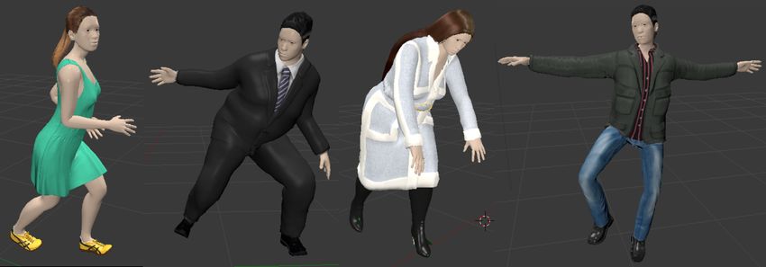
4       Martı́nez-González A., Villamizar M., Canévet O. and Odobez J.M.

seek to align the data distributions by minimizing the distance between domains pro-
vided domain distribution parametrizations [7]. On the other hand, current deep learning
methods make use of various training strategies and network architectures to ensure and
ease domain confusion and to automatically learn an invariant representation of the data
[8,4,16,26,27].
    For example [8] proposes to learn invariant data features in a multi-task adversarial
setting for object classification. The method learns jointly an object class and domain
predictors with shared features among the tasks. Domain adaptation is achieved by an
adversarial domain regularizer which aims at fooling the domain classifier, which is
in charge of predicting the domain the data comes from. The process encourages the
learning of features that makes the domain classifier incapable of distinguish between
domains.
    Domain adaptation has also been used for the task of 3D pose estimation from RGB
images [5]. The approach uses computer graphics software to synthesize colored and
textured images of humans that are subsequently merged with natural images as back-
ground. Domain adaptation is performed in a two step learning process by alternating
the updates of a domain predictor and pose regressor.
    Deep domain adaptation in the depth image domain is less covered in the literature.
A comparison of state-of-the-art domain adaptation techniques applied to object classi-
fication from depth images is presented in [19]. Along the same direction, a method for
feature transfer from the real to the synthetic depth domain is presented in [22].
    Although deep domain adaptation techniques have obtained remarkable results in
transferring domain knowledge, in the majority of the problems the visual domains
mainly differ in the objects perspective, lighting, background, and objects are mostly
image centered. In addition, most of the final tasks are image classification leaving an
open door to apply the same methods for regression problems and object localization
tasks, e.g. keypoint detection.

(a)                (b)     (c)                  (d)                (e)
Fig. 2: (a) Examples of the 3D characters we use for depth image synthesis, (b) skele-
ton model we follow to perform pose estimation, (c) examples of rendered synthetic
images, (d) color labeled mask, (e) examples of training images combining synthetic
depth silhouettes and real depth background images.

3     Depth Image Domains

This section presents the depth image domains we consider for our pose estimation
approach. First, we describe our approach to generate synthetic depth images for multi-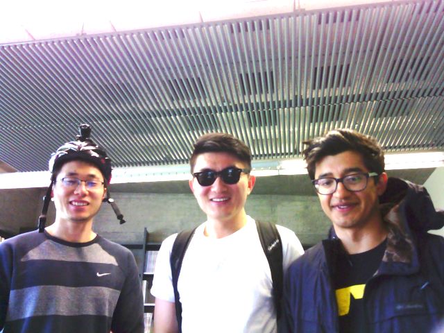
Investigating Depth Domain Adaptation for Efficient Human Pose Estimation      5

person pose estimation settings. Then, we introduce the target data for testing composed
of real depth image sequences recorded in a Human-Robot Interaction (HRI) scenario.

3.1   Synthetic Depth Image Generation

Training CNNs requires large amounts of labeled data. Unfortunately, a precise manual
annotation of depth images with body parts is troublesome, given that people roughly
appear as blobs.
    As mentioned before, synthesizing depth images is easier than color images due to
the lack of texture, color and lighting. We consider the synthetic depth image database
generated by the randomized synthesis pipeline proposed in [17]. The dataset contains
images displaying single person instances with different body pose and view perspec-
tives. Yet, it may not be well suited for learning multi-person pose estimation settings
like in HRI where people occlusion occur frequently. The data must then reflect these
cases. Building upon [17], we improve such pipeline to synthesize depth images dis-
playing two people under different pose configurations, and to extract high quality an-
notations. The synthesis pipeline is briefly described below.
Variability in body shapes. We consider a dataset of 24 3D characters that show varia-
tion in gender, heights and weights, and have been dressed with different clothing outfits
to increase shape variation (skirts, coats, pullovers, etc.).
Synthesis with two people instances. We cover the scenarios of multi-person pose
estimation by adding two 3D characters to the rendering scene. During synthesis, two
models are randomly selected from the character database and placed at a fixed distance
between each other. To avoid checking for collision between the characters we set a
minimum distance between them during rendering
Variability in body poses. Motion simulation is used to add variability in body pose
configurations. We perform motion retargeting from motion capture data sequences
taken from the CMU labs Mocap dataset [1].
Variability in view point. A camera is randomly positioned at a maximum distance of
8 meters from the models, and randomly oriented towards the models torso.
Dataset and annotations. The generated image dataset displaying two people instances
is publicly available as an extension of the data presented in [17]. Altogether, the two
datasets contain 223,342 images of people performing different types of motion un-
der different viewpoints with 51,194 images displaying two people. We automatically
extract the location of 17 body landmarks (head, neck, shoulders, elbows, wrists, hips,
knees, ankles, eyes) in camera and image coordinates. Keypoint visibility labels are also
provided. In addition, we extract color labeled silhouette masks for images that contain
two people instances. See Figure 2(b) for some examples.

3.2   Real Depth Image Domain Data

Depth imaging is generated as triangulation process in which a series of laser beams
are cast into the scene, captured by an infrared camera, and correlated with a reference
pattern to produce disparity images and finally the distance to the sensor. The image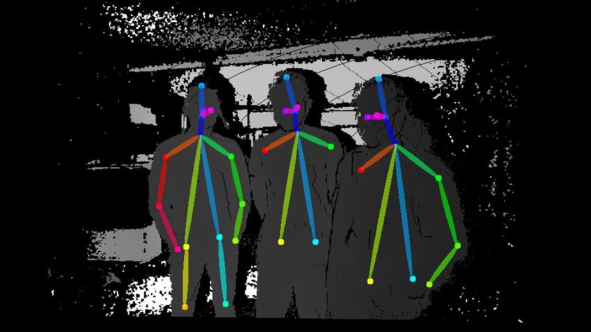
6          Martı́nez-González A., Villamizar M., Canévet O. and Odobez J.M.

(a)                                       (b)
Fig. 3: Depth imaging characteristics. (a) visual characteristics around the human sil-
houette in depth sensing are difficult to synthesize and therefore not present in the ren-
dered image, (b) HRI scene recorded with different RGB-D cameras, left to right: Intel
D435, Kinect 2 and Asus Xtion. Different depth sensors makes the recorded depth im-
ages to show specific type of visual characteristics for each sensor.

quality and visual features greatly depend on the sensor specifications, e.g. measure-
ment variance, missing data, surface discontinuities, etc. It is therefore natural to han-
dle depth-based pose estimation learning from synthetic data as a domain adaptation
problem, where each depth sensor type constitutes a domain.
    We study the problem of depth domain adaptation considering synthetic depth imag-
ing as the source domain and Kinect 2 depth imaging as the target domain. We further
focus in HRI settings and consider two datasets.
    First, we consider the Watch-n-Patch (WnP) database introduced in [30] which will
be used for adaptation purposes. To evaluate the performance of our method, we need a
second dataset. To this end, we conducted a series of data collection, recording videos
of people interacting with a robotic platform. The recorded data consist of 16 sequences
in HRI settings recorded with a Kinect 2. Each of the sequences has a duration of up
to three minutes and is composed of pairs of registered color and depth images. The
interactions were performed by 9 different participants in indoor settings under different
background scene and natural interaction situations. In addition the participants were
asked to wear different clothing accessories to add variability in the body shape. Each
of the sequences displays up to three people captured at different distance from the
sensor. In our experiments we refer to this recorded data as RLimbs. Both datasets with
annotations, synthetic and recorded HRI sequences, are publicly available 1 .
    In Section 5 we show how to use this data to bridge the gap between synthetic and
real depth image domains, improving the pose estimation performance in real images
without the need of annotations on the real data.

4      Depth Domain Adaptation for Pose Estimation

Our pose estimation approach is inspired in the convolutional pose machines (CPM)
framework [3]. That is, we predict body parts and limbs of multiple people in a cascade
of detectors fashion. In this section we describe the base CNN architecture we follow
for pose estimation and the modifications we add to perform depth domain adaptation.
 1   https://www.idiap.ch/dataset/dih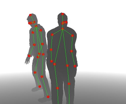
Investigating Depth Domain Adaptation for Efficient Human Pose Estimation                                                                               7

4.1     Base CNN Architecture and Pose Learning

              (a) Feature Extractor                                                           (b) Pose regression cascade

                                                                                                   3x3 3x3 3x3 1x1   1x1              7x7 7x7 7x7   7x7 7x7 1x1 1x1

      Depth
      Image
               7x7        3x3   3x3   +     3x3   3x3   +            3x3   3x3   +    1x1

                                                                                                   3x3 3x3 3x3 1x1   1x1              7x7 7x7 7x7   7x7 7x7 1x1 1x1

                       Residual Module 1 Residual Module 2        Residual Module 3

                     7x7 Convolution                             Fully Connected
                     3x3 Convolution                         +   Addition                         (c) Domain classi er
                     1x1 Convolution                             Concatenation
                     2x2 Average Pooling
                                                                                            GRL              1x1           1024   1
              GRL
                     Gradient Reversal Layer

Fig. 4: Architecture design of the CNN used for pose estimation from single channel
depth images. The base architecture is composed of a feature extractor module (a),
and a pose regression cascade (b). The architecture is further extended with a domain
classifier (c) for depth domain adaptation.

Pose Regression CNN Architecture. Figure 4(a) and (b) comprise the base architec-
ture of the pose regression network used to detect body parts and limbs, taking as input
a single channel depth image.
     Specifically, the neural network architecture is composed of a feature extractor mod-
ule GF (·) parametrized by θF , and a pose regression cascade module Gy (·) parametrized
by θY . For an input depth image x the feature extractor module computes a compact im-
age representation (features) Fx = GF (x) that is internal to the network. This internal
image representation Fx is then passed to the pose regression cascade module GY (·) in
order to localize body parts and limbs according to our skeleton model (Figure 2(b)).
     A predictor t in the pose regression cascade consist on two branches of fully convo-
lutional layers. Branch ρt (·) performs the task of body part detection, whereas branch
φt (·) localizes body limbs. By considering a number of sequentially stacked detectors,
the body parts and limbs predictions are refined using the result of previous stages and
incorporating image spatial context through the features Fx .
     Finally, pose inference is performed in a greedy bottom-up step to gather parts and
limbs belonging to the same person, as originally proposed by the CPM framework.
Feature Extractor Module. The network’s feature extraction module GF (·) computes
the image features Fx by applying a series of residual modules to the image x. The
architecture of GF (·) comprises three residual modules with small kernel sizes and
three average pooling layers. Batch normalization and ReLU are included after each
convolutional layer and after the shortcut connection.
    The architeture of GF (·) has been designed targeting efficient and fast forward pass,
relying on the representational power and efficiency of residual modules. The combina-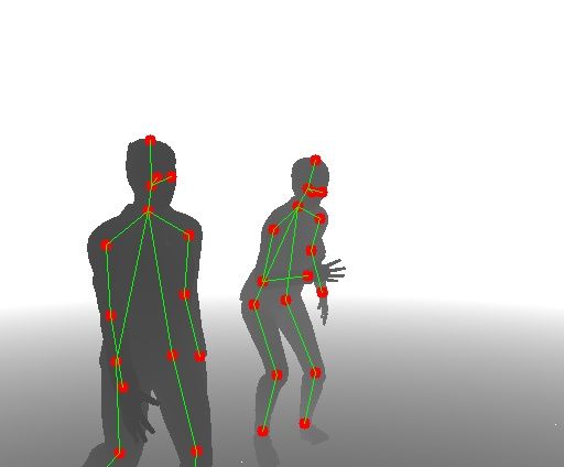
8       Martı́nez-González A., Villamizar M., Canévet O. and Odobez J.M.

tion of the processing time taken by the feature extractor together with the cascade of
detectors can provide estimations at a frame rate of 35 FPS.
Pose Regression Module. In the pose regression cascade module, each stage t takes as
input the image features Fx and the output of the previous detector t − 1. As depicted on
Figure 4(b), a detector consists of two branches of convolutional layers, the first branch
predicting the location of the parts, and the second predicts the location and orientation
of the limbs. Note that with only one stage there is no refinement since the first stage
only takes as input the features Fx .

Confidence Map Prediction and Pose Regression Loss. We regress confidence maps
for the location of the different body parts and predict vector fields for the location and
orientation of the body limbs.
    The ideal representation of the body part confidence maps S∗ encodes the ground
truth location on the depth image as Gaussian peaks. The ideal representation of the
limbs L∗ encodes the confidence for the connection between two adjacent body parts,
in addition to information about the orientation of the limbs by means of a vector field.
We refer the reader to [17] for more details on the generation of the confidence maps.
    We define the pair of body parts and body limbs ideal representations as Y = (S∗ , L∗ ).
Intermediate supervision is applied at the end of each prediction stage to prevent the net-
work from vanishing gradients. This supervision is implemented by two L2 loss func-
tions, one for each of the two branches, between the predictions St and Lt and the ideal
representations S∗ and L∗ . The loss functions at stage t are

             ft1 =   ∑ ||St (p) − S∗ (p)||22 ,    ft2 =   ∑ ||Lt (p) − L∗ (p)||22 .    (1)
                     p∈I                                  p∈I

The pose regression loss is computed as LY = ∑t=1T
                                                   ft1 + ft2 where T is the total


number of stages in the pose regression cascade.

4.2   Depth Domain Adaptation

Ideally, testing and training depth images should live in the same domain. In our case,
learning a pose regression network from synthetic data limits its generalization capacity
given the missing real depth image details not present in the synthetic training set. We
perform domain adaptation to map synthetic and real images to a representation that
is similar across domains. We follow closely the method presented in [8] for domain
adaptation and adapt it to our body part localization setting.
    For our unsupervised domain adaptation learning algorithm we are given a source
distribution sample (synthetic depth image dataset) S = {(xi , yi )}Ni=1 ∼ DS and a tar-
get dataset sample (real depth image dataset) T = {xi }M   i=1 ∼ DT . We are only given
annotations of 2D keypoint locations yi for the source distribution samples xi .
    The distance between the source and target distributions can be measure via the H-
divergence [8]. Although this is impractical to compute, it can be approximated by the
generalization error of the problem of domain classification. In essence, the distance
between distributions is minimum if the domain classifier is incapable of distinguishing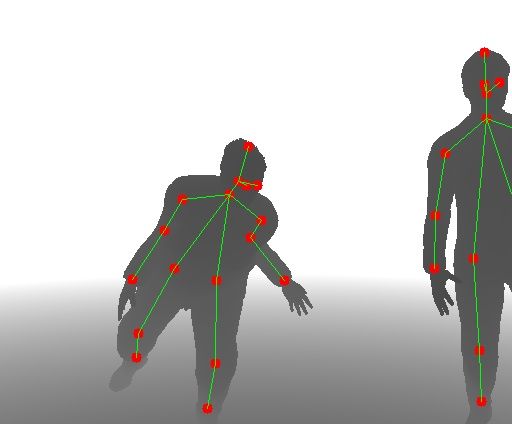
Investigating Depth Domain Adaptation for Efficient Human Pose Estimation        9

between the different domains. Therefore, to achieve domain confusion, the data need
to be mapped to a representation that is invariant, or at least indistinguishable, across
domains.
    Let Fx be the internal representation of image x in the network (features) computed
as Fx = GF (x) for a feature extractor GF (·). A measure of domain adaptation is com-
puted by
                              1                     1
                    Ld = −       ∑ ld (Gd (Fx )) − |T | ∑ ld (Gd (Fx )),              (2)
                             |S| x∈S                    x∈T

where and ld is a logistic regression loss, and Gd is a domain classifier, parametrized by
θd , such that Gd (Fx ) = 1 if x ∈ T and 0 otherwise.
     In the problem of domain classification, the domain classifier Gd (·) is fooled when
GF (·) produces equivalent features for both domains. A feature extractor capable of
producing such type of features is learned by maximizing Eq (2)

                                      Rd = max Ld .                                     (3)
                                              θd

    Eq (3) aims to approximate the empirical H- divergence between domains S and T
as 2(1 − Rd ).

4.3   Joint Pose Learning and Adaptation

The pose learning and domain adaptation joint optimization objective can be written as

                                     L = LY + λ Rd ,                                    (4)

where λ is a parameter that tunes the trade-off between the pose learning and domain
adaptation. The second term of Eq (4) acts as a domain regularizer.
    Our pose regression network shown in Figure 4(a) and (b) naturally provides the
scheme for the joint learning and adaptation problem via a domain classifier (Fig-
ure 4(c)). We implement the domain classifier via a neural network composed of two
average pooling layers with an intermediate layer of 1 × 1 convolution and followed by
two fully connected layers that produces a sigmoid function. As shown in Figure 4 both
the pose regression cascade GY (·) and the domain classifier Gd (·) receive as input the
features generated by GF (·).
    The learning and adaptation problem stated by Eq (4) proposes an adversarial learn-
ing process which involves a minimization with respect to the pose regression loss LY
and a maximization with respect to the domain classifier regularizer Rd . We follow [8]
by including a gradient reversal layer (GRL) in the architecture to facilitate the joint op-
timization. The GRL acts as identity function during the forward pass of the network,
but reverses the direction of the gradients from the domain classifier during backpropa-
gation.
    The nature of pose regression and domain adaptation problems makes the losess
involved in Eq (4) to live in different ranges. Therefore, the trade-off parameter λ has
to reflect both the importance of the domain classification regularizer as well as to this
difference between ranges.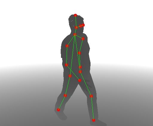
10      Martı́nez-González A., Villamizar M., Canévet O. and Odobez J.M.

5     Experiments and Results
In a series of experiments we show how different datasets, recorded with the same type
of sensor, are used to improve pose estimation via unsupervised domain adaptation. In
this section we analyze the performance obtained under different modeling selections
on the network architecture and domain adaptation configurations.

5.1   Data

Synthetic domain data. We split the synthetic dataset into three folds with the follow-
ing percentage and amount of images: training (85%, 189,844), validation (5%, 11,165),
and testing (10%, 22,333).
Synthetic training data augmentation. We add the following perturbations to the syn-
thetic images to add realism and avoid overfitting to synthetic clean details.
Adding real background content. We consider the dataset in [14] containing 1,367 real
depth images recorded with a Kinect 1 and exhibiting depth indoor clutter. During learn-
ing, training images were produced on the fly by randomly selecting one depth image
background and body synthetic images, and composing a depth image with background
using the character silhouette mask. Sample results are shown in Figure 2(d).
Pixel noise. We randomly select 20% of the body silhouette’s pixels and set their value
to zero.
Image rotation. Training images are rotated with a probability 0.1 by a randomly se-
lected angle in the range [−20, 20] degrees.
Real domain data. Our real domain consist Kinect 2 data. We use the data presented
in Section 3.2 to perform domain adaptation. The Watch-n-Patch dataset was used for
adaptation purposes only. We randomly select 85% out of the total number of images
comprised over all the sequences, leading to a total of 66,303 depth.
    We used the RLimbs data for training, validation and testing purposes. We divide
the data taking into account clothing features, actor ID and interaction scenario, in such
a way that an actor does not appear in the training and testing sets under similar circum-
stances. The train, validation and test folds consist of 7, 5 and 4 sequences respectively.
We annotate small sets from each fold to be used for validation (750 images), testing
(1000 images) and fine-tuning (1750 images).

5.2   Evaluation protocol

Accuracy metric. We use standard precision and recall measures derived from the Per-
centage of Correct Keypoints (PCKh) as performance metrics [31]. More precisely, we
extract landmark predictions p whose confidence is larger than a threshold τ. Pose esti-
mates are generated from these predictions by the part association algorithm. Then, for
each landmark type we associate the closest prediction p whose distance to ground truth
q is below a distance threshold d = κ × h, where h stands for the height of the ground
truth bounding box of the person to which q belongs to. The associated predictions p
count as true positives and the rest as false positives. Ground truth points q with no
Investigating Depth Domain Adaptation for Efficient Human Pose Estimation 11
associated prediction are counted as false negatives. The average recall and precision
values can then be computed by averaging over the landmark types and then over the
dataset. Finally, the average recall and precision values used to report performance are
computed by averaging the above recall and precision over several distance thresholds
by varying κ in the range [0.05, 0.15].
5.3 Implementation details
Pose regression network We use Pytorch as the deep learning framework in all our ex-
periments. First, we train our pose regression network (Figure 4(a) and (b)) on synthetic
data with stochastic gradient descent with momentum during 300 K iterations. We set
the momentum to 0.9, the weight decay constant to 5 × 10⁻⁴ , and the batch size to 10.
We uniformly sample values in the range [4 × 10⁻¹⁰ , 4 × 10⁻⁵ ] as starting learning rate
and decrease it by a factor of 10 when the validation loss has settled. All networks are
trained from scratch and progressively, i.e. to train network architectures with t stages,
we initialize the network with the parameters of the trained network with t − 1 stages.
We consider network architectures with pose regression cascade modules comprised by
upto 2 prediction stages.
Domain adaptation. After training the pose regression network for some time with
synthetic data, we run the domain adaptation process. The adaptation is performed for
T = 100 K iterations. We monitor and select models according to the lowest value of a
validation loss computed on the RLimbs validation set. The learning rate parameter is
kept fixed to the last value in the previous training procedure. Domain classifier param-
eters are randomly initialized using a Gaussian distribution with mean zero and small
variance.
We opt to gradually adapt the trade-off parameter λ of eq (4) according to the train-
ing progress as
2Λ
λp = −Λ, (5)
1 + exp(−10p)
where p = t/T for the current iteration progress t. The constant Λ was experimentally
chosen in order to accommodate both losses in eq (4) in the same range. In our experi-
ments we observed a good behavior of pose learning and adaptation for Λ = 100.
Model notation. We analyze CNN architectures with 1 and 2 prediction stages in the
pose regressor cascade. In our results we refer to this configurations as RPM1S and
RPM2S respectively. Postfixes -DA and -FT are added whenever used domain adapta-
tion or fine-tuning respectively.
5.4 Results
Domain Adaptation and Network Configuration. We analyze the impact of domain
adaptation on the different levels of prediction stages. For these experiments we con-
sider the Watch-n-Patch data for the adaptation process and the RLimbs data for testing.
The models were trained as follows. First, a single stage network was trained with syn-
thetic data and then with domain adaptation. Next, a network architecture with 2 stages12 Martı́nez-González A., Villamizar M., Canévet O. and Odobez J.M.
1.00
1.00
1.00
0.95
0.95
0.95
Average Precision
Average Precision
Average Precision
0.90
0.90
0.90
0.85
0.85
0.85
RPM1S RPM2S RPM2S
RPM2S RPM2S-DA t=300k RPM2S+FT
RPM1S-DA RPM2S-DA t=200k RPM2S-DA
RPM2S-DA RPM2S-DA t=150k RPM2S-DA+FT
0.80
0.80
0.80
0.0 0.2 0.4 0.6 0.8 0.0 0.2 0.4 0.6 0.8 0.0 0.2 0.4 0.6 0.8
Average Recall Average Recall Average Recall
(a) (b) (c)
Fig. 5: Average recall-precision curves. (a) impact when applying domain adaptation at
the different levels of prediction stages. (b) performance for different starting points of
domain adaptation. (c) comparison of domain adaptation and fine-tuning.
100 100
90 90
80 80
70 70
Precision (%)
60 60
Recall (%)
50 50
40 40
30 30
20 20
RPM2S RPM2S
10 10
RPM2S-DA RPM2S-DA
0 0
LWrist
RWrist
LWrist
RWrist
Neck
Head
TopHead
LEye
REye
LShoulder
RShoulder
LElbow
RElbow
LHip
RHip
LKnee
RKnee
LAnkle
RAnkle
Neck
Head
TopHead
LEye
REye
LShoulder
RShoulder
LElbow
RElbow
LHip
RHip
LKnee
RKnee
LAnkle
RAnkle
Fig. 6: Recall (left) and precision (right) per body part before and after domain adapta-
tion. Note the high gain in recall for lower body parts after applying domain adaptation.
was trained on synthetic data taking the single stage adapted network as initial point.
Finally domain adaptation is performed.
The resultant average recall-precision curves are presented in Figure 5(a). We ob-
serve that domain adaptation improves mainly the recall performance at the two levels
of prediction stages. Including spatial context via a second prediction stage is vital. Ta-
ble 1 summarizes these results reporting the models with the largest F1-Score in the
curves. The table also shows the performance on the upper-body. In Figure 6 we show
a comparison of the per body part precision and recall before and after adaptation. Do-
main adaptation mainly improves the recall on the lower body parts. As depicted in
Figure 3, these parts are the main components in the body silhouettes affected by noise
and sensing failures.
Domain Adaptation Starting Point. We conducted experiments in order to find the
best training point to start the domain adaptation process. To this end, we start domain
adaptation at different points of the synthetic training progress for the RPM2S model.
We selected starting points at t = 150K, t = 200K and t = 300K training iterations.
Figure 5(b) shows the performance of the different learned models. We note the perfor-
mance among the different runs remains the same. However, the earliest starting point
considered show more stable behavior.Investigating Depth Domain Adaptation for Efficient Human Pose Estimation 13
Performance
All body Upper body
Architecture AP AR AP AR
RPM1S 83.55 39.20 85.98 55.86
RPM1S-DA 83.68 48.56 89.39 68.63
RPM2S 91.56 53.47 93.93 69.93
RPM2S-DA 92.62 61.66 95.00 76.09
Table 1: Comparison of the performance (%) on the RLimbs test set for architectures
with different number of prediction stages before and after domain adaptation.
RLimbs based Domain Adaptation. As mentioned before, it is natural to think a
depth sensor as a generating domain. We perform domain adaptation using the training
fold of the RLimbs database as the target domain sample. As before, we start domain
adaptation at different points of the synthetic training and report the model results with
the best F1-Score. Table 2 compares the obtained performances. In the table we specif-
ically show the dataset used as target sample during the adaptation process, the source
data and the testing data. Note that using both Kinect 2 datasets in the adaptation process
improves the performance. Adaptation with the Watch-n-Patch dataset provides slightly
better results. It is worth to notice that the number of recorded scenarios, people, and
view points contained in the Watch-n-Patch is larger than those contained the RLimbs
dataset. This variability is somehow useful in the adaptation process. We include the
performance obtained by preprocessing the image with a simple in-paint process. This
technique was previously used to alleviate the discontinuities inherited from depth sens-
ing for non adapted models [17]. However, this lowers the precision score with a very
little gain in accuracy.
Fine-Tunning. To understand the limits of adapting between depth domains, we per-
formed fine-tunning on an annotated subset of the RLimbs dataset. We considered both,
the models trained with synthetic data and adapted models. Figure 5(c) shows the de-
tailed recall- precision curves. As expected, fine tuning on the target data provides bet-
ter generalization capabilities. However, fine-tuning on models with previous adapta-
tion show further improvement. Table 2 summarizes the results for the models with
the largest F1-Score. Figure 7 shows a qualitative comparison of the pose estimation
approach for adapted and not adapted models.
6 Conclusions
In this paper we investigated the use of unsupervised domain adaptation techniques
applied to the problem of depth-based pose estimation with CNNs. Specifically, we
investigated an adversarial domain adaptation method to improve the performance on
real depth images of a CNN-based human pose regressor trained with synthetic data. We
introduced a new dataset of synthetically generated depth images displaying two people
instances to cover cases of multi-person pose estimation. In addition, we presented a14 Martı́nez-González A., Villamizar M., Canévet O. and Odobez J.M.
Performance
Data All body Upper body
Source Target Testing AP AR AP AR
Synthetic — RLimbs 91.56 53.47 93.93 69.93
Synthetic — RLimbs (IP) 81.98 58.23 85.20 72.66
Synthetic WnP [30] RLimbs 92.62 61.66 95.00 76.09
Synthetic RLimbs RLimbs 92.32 59.32 95.05 74.55
Synthetic + FT — RLimbs 90.56 79.23 93.64 89.52
Synthetic + FT WnP [30] RLimbs 91.27 82.03 93.73 90.83
Synthetic + FT RLimbs RLimbs 91.03 78.98 94.32 89.32
Table 2: Top: comparison of performance (%) by using two different datasets of depth
images as the target data for domain adaptation. IP stans for in-paint preprocessing. Bot-
tom: performance obtained by fine tuning (FT) on an annotated subset of the RLimbs
training set after learning with synthetic data and after domain adaptation on the differ-
ent depth image datasets.
dataset containing videos of people in HRI scenarios. Both synthetic and real recorded
data are publicly available.
Our experiments show that different data from the same type of sensor is meaning-
ful to cover part of the performance gap introduced by learning from synthetic depth
images. However, devoting some effort to label a few examples maybe critical to in-
crease the model’s generalization capabilities. We observed that the combination of
both approaches, domain adaptation and fine tuning, increase performance. Suggesting
that domain adaptation for body pose estimation from depth images a better path to
follow is a semi-supervised approach.
ACKNOWLEDGMENTS
This work was supported by the European Union under the EU Horizon 2020 Research
and Innovation Action MuMMER (MultiModal Mall Entertainment Robot), project ID
688147, as well as the Mexican National Council for Science and Tecnology (CONA-
CYT) under the PhD scholarships program.
References
1. Cmu motion capture data. http://mocap.cs.cmu.edu/.
2. Adrian Bulat and Georgios Tzimiropoulos. Human pose estimation via convolutional part
heatmap regression. In ECCV, 2016.
3. Zhe Cao, Tomas Simon, Shih-En Wei, and Yaser Sheikh. Realtime multi-person 2d pose
estimation using part affinity fields. In CVPR, 2017.
4. Fabio Maria Carlucci, Lorenzo Porzi, Barbara Caputo, Elisa Ricci, and Samuel Rota Bulo.
Autodial: Automatic domain alignment layers. In International Conference on Computer
Vision (ICCV), 2017.Investigating Depth Domain Adaptation for Efficient Human Pose Estimation 15
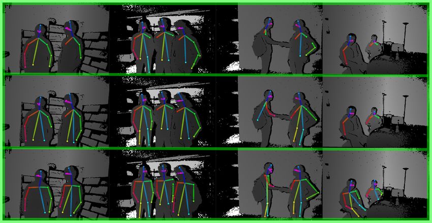
Fig. 7: Output of the different models for some images contained in the testing set of
RLimbs. Top row: pose estimation before domain adaptation. Middle row: pose estima-
tion after domain adaptation. Bottom row: pose estimation with fine tuning after domain
adaptation.
5. Wenzheng Chen, Huan Wang, Yangyan Li, Hao Su, Zhenhua Wang, Changhe Tu, Dani
Lischinski, Daniel Cohen-Or, and Baoquan Chen. Synthesizing training images for boosting
human 3d pose estimation. In 3D Vision (3DV), 2016.
6. Ben Crabbe, Adeline Paiement, Sion Hannuna, and Majid Mirmehdi. Skeleton-free body
pose estimation from depth images for movement analysis. In IEEE Conference on Computer
Vision and Pattern Recognition (CVPR), pages 312–320, 12 2015.
7. Gabriela Csurka. Domain adaptation for visual applications: A comprehensive survey. In
Domain Adaptation in Computer Vision Applications, chapter 1, pages 1–35. Springer Series:
Advances in Computer Vision and Pattern Recognition, 2017.
8. Yaroslav Ganin, Evgeniya Ustinova, Hana Ajakan, Pascal Germain, Hugo Larochelle,
François Laviolette, Mario Marchand, and Victor Lempitsky. Domain-adversarial training
of neural networks. J. Mach. Learn. Res., 17(1):2096–2030, January 2016.
9. Albert Haque, Boya Peng, Zelun Luo, Alexandre Alahi, Serena Yeung, and Li Fei-Fei. To-
wards viewpoint invariant 3d human pose estimation. In European Conference on Computer
Vision (ECCV), October 2016.
10. Peiyun Hu and Deva Ramanan. Bottom-up and top-down reasoning with hierarchical recti-
fied gaussians. In Proceedings of the 2016 IEEE Conference on Computer Vision and Pattern
Recognition, pages 5600–5609, 06 2016.
11. Eldar Insafutdinov, Mykhaylo Andriluka, Leonid Pishchulin, Siyu Tang, Evgeny Levinkov,
Bjoern Andres, and Bernt Schiele. Articulated multi-person tracking in the wild. In CVPR,
2017. Oral.
12. Eldar Insafutdinov, Leonid Pishchulin, Bjoern Andres, Mykhaylo Andriluka, and Bernt
Schieke. Deepercut: A deeper, stronger, and faster multi-person pose estimation model.
In European Conference on Computer Vision (ECCV), 2016.
13. Umar Iqbal, Anton Milan, and Juergen Gall. Posetrack: Joint multi-person pose estimation
and tracking. In IEEE Conference on Computer Vision and Pattern Recognition (CVPR),
2017.
14. Kourosh Khoshelham and Er Oude Elberink. Accuracy and resolution of kinect depth data
for indoor mapping applications. In Sensors 2012, 12, 14371454. 2013, page 8238, 2013.16 Martı́nez-González A., Villamizar M., Canévet O. and Odobez J.M.
15. Christoph Lassner, Javier Romero, Martin Kiefel, Federica Bogo, Michael J. Black, and Pe-
ter V. Gehler. Unite the people: Closing the loop between 3d and 2d human representations.
In The IEEE Conference on Computer Vision and Pattern Recognition (CVPR), July 2017.
16. Mingsheng Long, Han Zhu, Jianmin Wang, and Michael I Jordan. Unsupervised Domain
Adaptation with Residual Transfer Networks. In D. D. Lee, M. Sugiyama, U. V. Luxburg,
I. Guyon, and R. Garnett, editors, Advances in Neural Information Processing Systems 29,
page 136144. Curran Associates, Inc., 2016.
17. Angel Martı́nez-González, Michael Villamizar, Olivier Canévet, and Jean-Marc Odobez.
Real-time convolutional networks for depth-based human pose estimation. In 2018
IEEE/RSJ International Conference on Intelligent Robots and Systems, IROS 2018, 2018.
18. Alejandro Newell, Kaiyu Yang, and Jia Deng. Stacked Hourglass Networks for Human Pose
Estimation, pages 483–499. Springer International Publishing, Cham, 2016.
19. Novi Patricia, Fabio M. Cariucci, and Barbara Caputo. Deep depth domain adaptation: A
case study. In 2017 IEEE International Conference on Computer Vision Workshops, ICCV
Workshops 2017, Venice, Italy, October 22-29, 2017, pages 2645–2650, 2017.
20. Leonid Pishchulin, Eldar Insafutdinov, Siyu Tang, Bjoern Andres, Mykhaylo Andriluka, Pe-
ter Gehler, and Bernt Schiele. Deepcut: Joint subset partition and labeling for multi person
pose estimation. In IEEE Conference on Computer Vision and Pattern Recognition (CVPR),
2016.
21. J. Shotton, A. Fitzgibbon, M. Cook, T. Sharp, M. Finocchio, R. Moore, A. Kipman, and
A. Blake. Real-time human pose recognition in parts from single depth images. In Proceed-
ings of the 2011 IEEE Conference on Computer Vision and Pattern Recognition, CVPR ’11,
pages 1297–1304, Washington, DC, USA, 2011. IEEE Computer Society.
22. Ashish Shrivastava, Tomas Pfister, Oncel Tuzel, Josh Susskind, Wenda Wang, and Russ
Webb. Learning from simulated and unsupervised images through adversarial training. In
IEEE Conference on Vision and Pattern Recognition, CVPR, 2017.
23. Chenyang Si, Wei Wang, Liang Wang, and Tieniu Tan. Multistage adversarial losses for
pose-based human image synthesis. In The IEEE Conference on Computer Vision and Pat-
tern Recognition (CVPR), June 2018.
24. Karen Simonyan and Andrew Zisserman. Very deep convolutional networks for large-scale
image recognition. 2014.
25. Jonathan J Tompson, Arjun Jain, Yann LeCun, and Christoph Bregler. Joint training of a
convolutional network and a graphical model for human pose estimation. In Z. Ghahramani,
M. Welling, C. Cortes, N. D. Lawrence, and K. Q. Weinberger, editors, Advances in Neural
Information Processing Systems 27, pages 1799–1807. Curran Associates, Inc., 2014.
26. Eric Tzeng, Judy Hoffman, Trevor Darrell, and Kate Saenko. Simultaneous Deep Transfer
Across Domains and Tasks. In International Conference in Computer Vision (ICCV), 2015.
27. Eric Tzeng, Judy Hoffman, Trevor Darrell, and Kate Saenko. Adversarial Discriminative
Domain Adaptation. In Computer Vision and Pattern Recognition (CVPR), 2017.
28. Keze Wang, Shengfu Zhai, Hui Cheng, Xiaodan Liang, and Liang Lin. Human pose estima-
tion from depth images via inference embedded multi-task learning. In Proceedings of the
2016 ACM on Multimedia Conference, MM ’16, pages 1227–1236, New York, NY, USA,
2016. ACM.
29. Shih-En Wei, Varun Ramakrishna, Takeo Kanade, and Yaser Sheikh. Convolutional pose
machines. In CVPR, 2016.
30. Chenxia Wu, Jiemi Zhang, Silvio Savarese, and Ashutosh Saxena. Watch-n-patch: Unsuper-
vised understanding of actions and relations. In The IEEE Conference on Computer Vision
and Pattern Recognition (CVPR), June 2015.
31. Yi Yang and Deva Ramanan. Articulated human detection with flexible mixtures of parts.
IEEE Trans. Pattern Anal. Mach. Intell., 35(12):2878–2890, December 2013.You can also read