Interested in learning more? - Global Information Assurance Certification Paper
←
→
Page content transcription
If your browser does not render page correctly, please read the page content below
Global Information Assurance Certification Paper

                            Copyright SANS Institute
                            Author Retains Full Rights
   This paper is taken from the GIAC directory of certified professionals. Reposting is not permited without express written permission.

Interested in learning more?
Check out the list of upcoming events offering
"Intrusion Detection In-Depth (Security 503)"
at http://www.giac.org/registration/gcia
Faster Than a Speeding Bullet: Using Geolocation to
Track Account Misuse
GIAC GCIA Certification
Author: Tim Collyer, tccollyer@gmail.com
Advisor: Barbara Filkins
Accepted: November 17th 2014
Abstract
Today’s global economy and mobile workforce have a large impact on modern network
security, elevating the importance of a “defense in depth” approach. Geolocation
information has become an important element to monitor as part of such a layered
defense. Incorporating geolocation information into network security programs does not
necessarily require additional expenditure if the appropriate resources (such as a SIEM)
are already in place. By tracking the geographic location for account logins, it is possible
to discover anomalies by calculating the distance between two logins from the same
account. If the speed required to travel that distance within the allotted time is unlikely or
impossible, this can indicate account misuse. This use of geolocation data can augment
other monitoring techniques to detect malicious behavior on a network. This paper
explores how such calculations can be made, identifies parts of the process requiring
special consideration, and highlights what can be revealed when using geolocation data to
monitor account use.
Tim Collyer, tccollyer@gmail.com 1 1. Introduction
A well-established security program is based upon the principles of defense in
depth with numerous types of controls in place throughout the network. Each of these
systems provide alerts and logs notifying the security analyst of possible attacks or other
incidents.
The problem then moves from acquiring evidence of attacks to sifting through the
mountains of information flowing past analysts in such a way as to highlight the data of
interest. The first step to making sense of all the information is to send it to a single
collection spot, usually a device called a SIEM or Security Information and Event
Manager. The real benefit of a SIEM is not just as an aggregator of log data - there is still
far too much of it and far too much noise for any human to be able to make sense of it. A
quality SIEM provides a framework to apply logic to all of that data. This is where
correlation occurs and where the real value of log aggregation comes in.
A simple example of a SIEM correlation rule might be:
If these events occur in close proximity:
● The mail gateway sees a zip attachment
● the host-based AV for the email recipient sends an alert for malware
● the proxy sees outbound connection attempts to known-bad destinations
from that host
then send an alert to the Security Operations Center to examine the host.
This rule describes a possible event (i.e. someone received and opened an infected
email attachment and compromised their machine) by correlating between the logs from
multiple sources and sending actionable alerts to the team which should handle the
potential incident . This example is fairly straightforward as far as correlation rules go,
but illustrates how a SIEM might be used to automate log correlation.
Content or rule generation for the SIEM therefore becomes of primary importance
for a security program. All of the logs entering a SIEM represent large volumes of raw
Tim Collyer, tccollyer@gmail.com 2 data which can be refined into intelligence with the application of creativity and logic.
The use of geolocation data described in this paper is one such refinement. The
methodology described here is not intended to be revolutionary, but is an additional tool
for the security toolbox, and one which can be created through the use of existing
resources.
Geolocation information, the real-world location of an object, can be extracted
from IP addresses in several different ways. The concept of using that information as part
of “context aware security” (Gartner, n.d.) is simple to describe but some aspects can be
complex to actually implement. A common way to make use of geolocation data is to
look at the country level and determine if the network or company has any business
communicating with the destination country. Using more granular data (down to the city
level for example), additional possibilities open up. Common sense suggests that
something strange is going on if a user logs in from one city and then 15 minutes later
logs in from another city 3,000 miles away. Unless that user is endowed with
superpowers (e.g. faster than a speeding bullet), they are unlikely to have traveled those
3,000 miles in the space of 15 minutes and this event becomes something worth looking
into.
Targeted attacks against corporate or governmental networks often begin by
compromising an end user’s computer. This is where malware is often installed and
where most of the exploitation of vulnerabilities happens. In the “Cyber Kill Chain”
model described by Lockheed Martin (Hutchins et al., 2011), most of the steps can occur
on the end user workstation.
Figure 1 -Analysis of a successful intrusion, a.k.a. the cyber kill chain (Cloppert, 2010 )
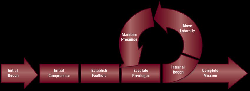
Tim Collyer, tccollyer@gmail.com 3 Ultimately, an attack against a network cycles through the kill chain more than
once as interim goals are achieved - first gaining a foothold on a network, then
maintaining persistence, finally locating and exfiltrating the data of interest. FireEye (Bu,
2014) illustrated the concept of looping through steps en route to the final goal with a
similar diagram to the kill chain:
Figure 2 - The attack lifecycle (Bu, 2014)
The first interim goal of the initial activity is often to obtain the valid credentials
of a user on the target network.The less malware used in the course of a compromise, the
lower the risk an attacker runs of being detected. Valid credentials permit an attacker the
opportunity to explore the network and find the targeted data - the looping steps in the
attack lifecycle diagram - possibly without introducing additional malware. Without
malware to cause alerts, or beaconing network traffic to a “command and control”
location (C2 in the kill chain diagram above), a security team must fall back on
behavioral analysis and context aware security.
Looking at geolocation data is one way to perform behavioral analysis.
Geolocation information may provide a way to identify accounts which have been
compromised and are being abused as part of an attack. It should be emphasized
however, that this type of analysis is examining the “Actions” phase of the kill chain.
Ideally, the kill chain would be disrupted much earlier in the process, but if initial
compromise has occurred, behavioral analysis can disrupt the next cycle through the kill
chain as the attack progresses towards its ultimate goal.
Tim Collyer, tccollyer@gmail.com 4 The concept of geolocation analysis to find account misuse is relatively simple to
describe but the implementation can be complex. Additionally, the events detected by this
type of data can be indicative of other forms of account misuse, besides that of
compromise, as will be discussed below.
The geolocation analysis occurs across three separate phases:
● Phase 1, Calculation - remote access logs are parsed and data is looked up
in the geolocation database to retrieve a location and timestamp
● Phase 2, Login Comparison - the raw data output from Phase 1 is
compared to derive geographic distance between logins and speed
required to traverse that distance
● Phase 3, Presentation - the output of the calculations is formatted and
presented in dashboard format for human review
Each phase is discussed below, reviewing the context around the phase as well as any
prerequisite data required. Then we examine the actual implementation within our
example SIEM, Splunk.
2. Input data
When preparing to compare account login locations and calculate whether it is
feasible for the user to have traveled between two points in the time between logins, a
variety of source data is required. They can be summarized as:
● Remote access logs (VPN logs which include source IP and login time are the
example used in this paper)
● Geolocation database
● Exclusion IPs
2.1 Remote access logs
Little needs to be said about the contents of the VPN logs, as the required data is
simple enough - a login IP and time, though additional information is often contained in
this type of log. The login IP should be a public IP address from which the remote user is
connecting. The timestamp must follow the same corollaries applied to log aggregation in
Tim Collyer, tccollyer@gmail.com 5 general, i.e. the time should be synchronized across the network and is probably most
easily handled if kept in UTC (i.e. Coordinated Universal Time, the main time standard)
to avoid time zone conversion errors. The importance of synchronized time cannot be
overstated. When tracking incidents and attempting to correlate events, as well as when
performing the geolocation analysis described here, piecing together the correct picture
relies on accurate timekeeping across disparate devices. The use of the Network Time
Protocol (NTP) is a common method to address this need. The mechanics of running
NTP or some other time correction mechanism across a network are outside the scope of
this paper, but it is a foundational element to any SIEM solution in order to provide
proper log correlation. Without synchronized time, the aggregated logs in a SIEM
become a messy hash of events that are out of order and need to be manually
reassembled.
2.2 Geolocation database
The geolocation database bears some additional explanation. Geolocation can be
determined from an IP address in a number of ways, depending upon available time,
money, and desired granularity. Probably the most common and most coarse method of
deriving some geolocation information from an IP address is by looking it up in a
WHOIS database and using the address of the registrar. As one might imagine, this leads
to rough results, depending upon the nature of the owner of the IP address. IP registration
data for a fairly small company might yield reasonably accurate information - almost
certainly the correct country, probably the correct state (if in the U.S), possibly the
correct city. However, a company the size of Google for example, which owns many IP
addresses, yields only limited value for geolocation purposes from the WHOIS
information. All of Google’s IP addresses would appear to be coming from Mountain
View, California, though Google clearly has many assets outside of Mountain View or
California or even the United States. A malicious registrant could even falsify the
registered address, sowing confusion and misinformation into the process.
What WHOIS lacks in detail, it makes up for in simplicity. For finer granularity
of resolution, more complex methods of data mining and other methods are required.
Tim Collyer, tccollyer@gmail.com 6 These include using traceroute and Border Gateway Protocol (BGP) routing tables to
determine the routing path and known location of backbone routers (Guo et al., 2009)
(Padmanabhan et al., 2001). It is also possible to analyze delay-based information, which
looks at the delay in connectivity between connections to IP addresses and attempts to
deduce geographic distance information from that delay (Wang et al., 2011). The
Worldwide Web Consortium (W3C) has even jumped into the game, offering a
geolocation API to provide a standardized interface to gather geolocation data from
client-side information.
The upshot of all of this is that getting accurate geolocation data is challenging
and painstaking work, gathering crumbs together until they can be assembled into a loaf
of bread so to speak. It is for this reason that many commercial services surrounding
geolocation data have sprung up, providing access to their database of gathered crumbs.
Among the several options for commercial geolocation information, IP2Location
(http://www.ip2location.com) and Maxmind (http://www.maxmind.com) are examples of
current leaders in the space. For the purposes of this paper, we will look at Maxmind.
Maxmind offers a free database which provides limited detail as well as a commercial
version which is more granular and frequently updated. The Maxmind FAQ has this to
say about the accuracy of the data:
“MaxMind tests the accuracy of the GeoIP Databases on a periodic basis. In our
recent tests, the GeoIP databases tested at 99.8% accurate on a country level, 90%
accurate on a state level in the US, and 83% accurate for cities in the US within a
40 kilometer radius.” (Maxmind, n.d.)
MaxMind also provides an accuracy web page which allows one to select
different levels of granularity to see the impact on accuracy across various countries
(https://www.maxmind.com/en/geoip2-city-accuracy). Regardless if the geolocation
information is a rough approximation or very fine-grained, any conclusions about account
misuse are absolutely reliant upon the completeness and accuracy of the data.
Tim Collyer, tccollyer@gmail.com 7 2.3 Exclusion lists
The other data set needed for accurate analysis is a list of IP addresses to be
excluded from the calculation. There are several reasons that an IP address might need to
be excluded from the geolocation calculation, but the most common has to do with
internet points-of-presence or gateways. The way that many large organizations design
their networks is to funnel all traffic out through specific gateways.
For example, consider a hotel chain. There are numerous different geographic
locations for hotels that are part of a chain, and each hotel has an IT infrastructure which
needs to be maintained, secured, and monitored. Duplicating all of the IT infrastructure
and security controls across hundreds or thousands of locations could be cost prohibitive
and an administrative nightmare to make sure that settings were consistent everywhere.
Instead, it might be much more efficient to funnel all internet traffic back to a small
number of gateways. Therefore the hotel in Reno, Nevada might be sending all of its
internet traffic back to corporate headquarters in, for example, Los Angeles, California.
So might all the other branches in Nevada, California, Utah, and Arizona. This allows the
IT and security departments to maintain centralized equipment at the corporate
headquarters, at the cost of probably unnoticeable latency increases for the hotel branch
user.
This is relevant to the discussion of geolocation because now any guest using the
WiFi offered by any branch of the hotel will appear to be having their traffic originate in
Los Angeles. This impacts the geolocation analysis significantly, rendering it all but
useless. A user might connect to the VPN from an IP which has valid geolocation data - a
small coffee shop in Salt Lake City for example - and then walk across the street and
check-in to the hotel and connect to the VPN from there. From our log analysis
perspective, it will appear that the user traveled from Salt Lake City to Los Angeles in a
few minutes, causing a false positive alert. Therefore networks with known architecture
along these lines must be part in the list of IP addresses to be excluded in order to reduce
false positives. Unfortunately, this also opens a large hole in the geolocation analysis.
Any malicious activity or account misuse which takes place within the exclusion list
Tim Collyer, tccollyer@gmail.com 8 networks will be ignored, leading to false negatives. There is not an existing good
solution to this conundrum, it is merely a flaw which should be understood before relying
upon these data. Almost all processes have flaws and assumptions, but that fact alone
does not mean that they need to be discarded. Rather, it is most important to understand
the shortcomings so as not to overstate the completeness of the results.
2.4 Phase 1, Calculation
With the input data in hand, it is possible to perform the first step in the analysis.
The VPN login information may well need to be de-duplicated, depending upon how the
VPN devices output the log data. Then the login IP addresses can be scrubbed against an
entry in the exclusion list. The scrubbed list of IP addresses can then be looked up in the
geolocation database and, finally, yield a login time, IP address, and geographic location.
This data will then be used in the next steps. The first phase of calculation is visualized in
the figure below.
Figure 3 - Logic flow to get geolocation data for VPN logins
2.5 Phase 1, Implementation
Now that the required input data has been explored and the general flow of data
through first stage of analysis described, it is valuable to provide a technical example of
how to implement the concepts. For the purposes of an example, the SIEM used will be
Splunk (www.splunk.com). Splunk offers a community version of the software which
Tim Collyer, tccollyer@gmail.com 9 provides full functionality but is limited on the amount of data which can be consumed
daily. Between the free version of Splunk and the free version of the Maxmind database,
the curious reader need only supply example VPN logs to be able to explore this
technique in a lab. Exclusion lists will need to be generated on a case-by-case basis
depending upon the nature and location of VPN traffic.
Thanks and acknowledgements go to Richard Gonzalez, a peer and friend in the
security industry who worked out (and agreed to share) the Splunk queries used to put the
geolocation analysis technique into practice (R. Gonzalez, personal communication,
September 3, 2014). The queries themselves get a bit complicated and though some
attempt will be made to describe the working parts, a deep explanation of how Splunk
works is outside the scope of this paper. Please note that part of implementing Splunk
involves naming data fields, sources, indices, etc. The flow of data through the Splunk
queries discussed is the important component and any specific naming conventions may
be changed as desired.
The Splunk query which matches the visualization diagram in Figure 3 is as
follows:
index=vpn NOT [|inputcsv public_exclusions_cidr.csv |
fields Public_IP] Public_IP=* | eval
username=upper(username) |dedup username, Public_IP,
Machine_Name | rename Public_IP as clientip| lookup
geoip | rename clientip as Public_IP| eval
client_city=coalesce(client_city, “Unknown”) | eval
client_country=coalesce(client_country, “Unknown”)| eval
client_region=coalesce(client_region, “Unknown”) | eval
formattedTime = strftime(_time, “%D %r”) | table
formattedTime,username,vpn_manager, Public_IP,
Machine_Name, client_city, client_region,
client_country, client_lat, client_lon
The breakdown is as follows:
● index=vpn NOT [|inputcsv public_exclusions_cidr.csv |
fields Public_IP] - this specifies the vpn logs which have been sent to
Tim Collyer, tccollyer@gmail.com 10 splunk and removes any IP addresses which match the exclusions listed in
“public_exclusions_cidr.csv”
● Public_IP=* | eval username=upper(username) |dedup
username, Public_IP, Machine_Name - performs some formatting to
make data easier to manipulate and then de-duplicates the VPN entries
● rename Public_IP as clientip| lookup geoip | rename
clientip as Public_IP - this portion of the query is passing the data to the
Maxmind Splunk app (https://apps.splunk.com/app/291/) and looking up the
geolocation data for each “Public_IP” object (renamed to clientip for the
Maxmind app)
● eval client_city=coalesce(client_city, “Unknown”) | eval
client_country=coalesce(client_country, “Unknown”)| eval
client_region=coalesce(client_region, “Unknown”) | eval
formattedTime = strftime(_time, “%D %r”) | table
formattedTime,username,vpn_manager, Public_IP,
Machine_Name, client_city, client_region, client_country,
client_lat, client_lon - First, this section populates all the fields which
had no data return from the geolocation database with the term “Unknown.” Then
some formatting occurs to provide the data in neat tabular form in preparation for
the next phase of analysis.
3. Phase 2, Login comparison
The first phase of geolocation analysis has provided a summary table of data
correlating usernames, IP addresses, geographic location, machine name, and time of
login. To complete the analysis we need to monitor this table for a specified period of
time looking for duplicate username entries and calculating the speed required to cover
the distance between the two locations within the allotted time. This seems relatively
simple, though there are some important details to factor in.
The first is the fact that the shortest distance between two points is not a straight
line when one lives on the surface of a sphere. Maps of the Earth are projections of a
three-dimensional object onto a two-dimensional surface. This results in some distortions
Tim Collyer, tccollyer@gmail.com 11 to which we have collectively grown accustomed. Those distortions mean that measuring
the distance between two cities on a map with a ruler (i.e. a straight line distance) will not
yield an accurate distance. The diagram below illustrates the fact that the straight red line
is clearly not the distance a person would be required to travel to get from point A to B,
unless they were to tunnel through the Earth. The arc between A and B is also known as
an orthodromic distance, or great circle distance.
Figure 4 - The black line is the shortest distance between two points on a sphere - a
“great circle” or orthodromic distance
Orthodromic distances are calculated frequently by aviators and mariners, or at
least by their navigation devices, to provide the shortest path to a destination. To maintain
reasonable accuracy in our distance calculations, we need to calculate the orthodromic
distance between VPN login locations. This calculation uses spherical trigonometry and
can appear a bit dense to pull apart:
a = sin²(Δφ/2) + cos φ1 ⋅ cos φ2 ⋅ sin²(Δλ/2)
c = 2 ⋅ atan2( √a, √(1−a) )
d = R ⋅ c
Figure 4 - The haversine equation, where φ is latitude, λ is longitude, and R is
earth’s radius (mean radius = 6,371km) (Verness, n.d.)
Tim Collyer, tccollyer@gmail.com 12 Happily, we work in the world of computers where such equations can be handled
simply and easily, so the details of spherical trigonometry will be left for another time.
Our example SIEM, Splunk, has an app called “haversine” which is designed to perform
just this calculation (https://apps.splunk.com/app/936/#/overview). It is nevertheless
worthwhile to have some understanding of exactly what is happening when stepping
through geolocation analysis. Understanding of the foundation helps to troubleshoot
problems with the data and interpret the results more accurately. Essentially all of that
spherical trigonometry boils down finding the length of a side of a triangle where that
side is a curve (e.g. the surface of the earth).
Figure 5 - trigonometry helps to solve for ‘c’ in a standard triangle (right), the haversine
formula uses spherical trigonometry to solve for ‘c’ when it is an arc (left)
3.1 Phase 2, Implementation
The Phase 1 calculation populated a “summary index” in Splunk which is a
method that Splunk provides for storing computationally intensive data. Summary indices
allow for quick data retrieval and use in subsequent calculations. Some of the technical
details about using Splunk, such as how to save data to a summary index, are not in scope
for this paper. Suffice it to say that the data from Phase 1 is being stored in a summary
Tim Collyer, tccollyer@gmail.com 13 index which, for clarity, has been named “IP mapping - Public IP to username with
location” in the Splunk query for Phase 2.
Now that we have our geolocation and login time from Phase 1 and the capability
to calculate the distance between two login locations via the haversine formula, we can
convert that distance into speed by dividing the distance by the time. That is all done with
the following Splunk query:
index=ip* source="IP mapping - Public IP to username
with location" Machine_Name=* |dedup username,
Public_IP, Machine_Name| eval location=client_city.",
".client_region.", ".client_country.", ".Public_IP.",
".Machine_Name| strcat client_lat "," client_lon latlon
|stats last(latlon) as latlon2, first(latlon) as
latlon1, last(location) as location2, first(location) as
location1, first(Machine_Name) as Machine1,
last(Machine_Name) as Machine2,first(search_now) as
time1, last(search_now) as time2,dc(latlon) as
distinctCount by username | where distinctCount = 2
|haversine units=mi originField=latlon1 latlon2|eval
time_diff=((time1-time2)/60)/60|eval
speed=distance/time_diff |where Machine1!=Machine2 |sort
distance desc
As before, here is the breakdown:
● index=ip* source="IP mapping - Public IP to username with
location" Machine_Name=* - This portion of the query is pulling the data
from the phase 1 summary index and only returning entries which have a
Machine_Name field that is populated (the “Machine_Name=*” portion will
exclude blank entries).
● dedup username, Public_IP, Machine_Name - A quick deduplication
of data entries
● eval location=client_city.", ".client_region.",
".client_country.", ".Public_IP.", ".Machine_Name - this
section creates a new field entitled “location” which is the collection of city,
region (state), country, public IP, and machine name data.
Tim Collyer, tccollyer@gmail.com 14 ● strcat client_lat "," client_lon latlon - the srtcat function
concatenates string values (Splunk, n.d), in this case connecting the user latitude
and longitude together as a single variable ‘latlon’ which is how the haversine app
requires input to be formulated
● stats last(latlon) as latlon2, first(latlon) as latlon1,
last(location) as location2, first(location) as location1,
first(Machine_Name) as Machine1, last(Machine_Name) as
Machine2,first(search_now) as time1, last(search_now) as
time2, - this section is moving data around and renaming it for ease of
comparison later. This section takes the first and last occurrence of various data
points (latlon, machine name, etc.) and renames them with distinct names (e.g.
latlon1 and latlon2).
● dc(latlon) as distinctCount by username | where
distinctCount = 2 - in terms of the phrasing in the query, the ‘dc(latlon)
as distinctCount by username’ section was actually part of the previous ‘stats’
section. However it seemed to make more sense to discuss all the distinct count
manipulation together. This portion of the query is looking for the number of
occurrences (distinct count) of latlon fields per username and then selecting those
that occur two times (‘where distinctCount = 2’) in preparation for the next
section.
● haversine units=mi originField=latlon1 latlon2 - This short
section is where the haversine formula is actually calculated using the haversine
app available for Splunk (https://apps.splunk.com/app/936/#/documentation). We
are specifying the units to be miles. As previously mentioned, the haversine app
requires the latitude and longitude to be formatted in a specific fashion, which
was done in the strcat section above.
● eval time_diff=((time1-time2)/60)/60|eval
speed=distance/time_diff - Here we’re calculating how much time
passed between logins and then using that to calculate the speed required to
traverse the distance in the specified time
Tim Collyer, tccollyer@gmail.com 15 ● where Machine1!=Machine2 - In an attempt to reduce false positives
stemming from artifacts of network architecture (e.g. the discussion on internet
gateways above), we have chosen to ignore any events where the name of the
machine is the same for each entry. Instead we are only looking at events with
different machine names but the same username.
● sort distance desc - A sort of the output in preparation for the next phase
of calculations
All of that data manipulation has a few caveats and assumptions which are worth
calling out. First of all, we are only only examining events with a distinct count of 2. This
means that if a user’s credentials appear in the data more than twice within the polling
period, it is ignored. This was done to minimize the complexity of an already complex
query process. Looking for occurrences of 3 or more login events and comparing them all
was deemed to be unnecessary with a short enough polling period. Accordingly, the
polling period (which is actually the Phase 1 query) is set to occur every 15 minutes.
Also, as mentioned above, we have chosen to discard events which occur where the
machine name is constant. This was done to reduce false positives, but could possibly be
leveraged as a way to avoid detection by an astute attacker.
4. Phase 3, Presentation of Results
We finally have all of the data required - the geolocation and time of VPN logins,
the distance and time between each login from the same username, and the speed
required to travel that distance within the time allotted. We now need to define when an
event requires an investigation and to display the data in a human-readable and usable
format. Here is a summary of the various thresholds/timing used in the course of these
calculations:
Calculation Threshold/Timing
Phase 1 query Runs every 15 minutes
Runs once per hour examining
Phase 2 query
previous 24 hours
Tim Collyer, tccollyer@gmail.com 16 Phase 3 query Runs when dashboard is invoked
Distinct count of VPN login events per 15 minutes 2
Max speed before alert 800 mph
Table 1 - various timing choices and thresholds defined to streamline the functionality of
data flow through the various queries
The threshold for speed, above which is considered to be an event worth
investigation, is an arbitrary value. Commercial airlines typically travel at speeds below
the speed of sound (Mach 1). Mach 1 varies based upon environmental conditions, but an
average value is approximately 760 mph (Benson, 2014). Therefore a value of 800 mph
was selected both for the fact that it is a round number and to allow for some margin of
error in the calculations. Under normal conditions, VPN users do not typically exceed the
speed of sound.
Here then is the final query used to populate the dashboard. As with Phase 1, the
Phase 2 data is stored in a summary index in this case named “Multi-machine VPN logins
- location and speed - daily.”
index=ip* daysago=2 source="Multi-machine VPN logins -
location and speed - daily" | dedup username, location1,
location2 | convert ctime(time1) as second_time |
convert ctime(time2) as first_time | rename location1 as
second | rename location2 as first | table username,
first_time,second, second_time,first, time_diff, speed |
where speed > 800 | sort speed desc | search NOT
first=*unknown* | search NOT second=*unknown*
Here is the breakdown:
● index=ip* daysago=2 source="Multi-machine VPN logins -
location and speed - daily" - pulls the Phase 2 summary index data
for the previous two days
● dedup username, location1, location2 - data deduplication
Tim Collyer, tccollyer@gmail.com 17 ● convert ctime(time1) as second_time | convert ctime(time2)
as first_time - the Phase 2 query invoked a function “search_now” which
returns time values in Unix epoch time (the number of seconds since 00:00:00
January 1, 1970). This portion of the query converts from epoch time to a more
human-readable and familiar format.
● rename location1 as second | rename location2 as first |
table username, first_time,second, second_time,first,
time_diff, speed | where speed > 800 | sort speed desc -
there are several actions occurring here, but they are easier to consider as a whole.
This section begins by renaming some values for more clarity in the table, it then
creates the table with the username, times, travel time, and speed. Finally it
selects any entries with a speed greater than 800 mph and sorts them by speed.
● search NOT first=*unknown* | search NOT second=*unknown* -
Finally, any entries which have “unknown” in them are discarded. “Unknowns”
arise from time to time due to bad lookup returns. They provide no useful data so
they are discarded.
We have now correlated VPN login information and geolocation data to allow us
to perform some account misuse detection. Here is an example of what the final
dashboard might look like (split into two images for legibility):
Figure 6 - Example (fictional) entries from the final dashboard “Abnormal VPN activity”
as displayed in Splunk
There are certainly other possibilities for dashboard output depending upon the
creativity and available time of the creator. For example, the geographic location could
Tim Collyer, tccollyer@gmail.com 18 be plotted on a map to provide a simple visual method to evaluate the information. For
simplicity’s sake, the dashboard discussed here is kept to native Splunk output and only
the essential information.
Originally the idea was to detect account misuse arising from compromised
credentials. And indeed that will show up in the results, but use of this process also
highlights another form of account misuse - credential sharing. Typically user accounts
are a method of authenticating a specific person so that appropriate permissions can be
applied to access the correct level of data. Therefore security policies often prohibit the
sharing of user account credentials, as this defeats the whole point of authentication.
Credential sharing in large network will be detected by this geolocation process, provided
that the users are geographically distant enough from each other. This makes sense -
credential sharing is just a voluntary form of account compromise - but it’s worth noting
because those types of events may be more likely in any given network than malicious
account compromise. This is in part due to the fact that there are specific defenses to
protect against account compromise, whereas there are fewer controls to prevent,
prohibit, or detect credential sharing. A security team implementing this geolocation
process should anticipate the addition of credential sharing incidents to the workload.
Though not the original aim of the process, detection of credential sharing provides
additional value to a security team looking to find unusual activity and enforce security
policies.
5. Conclusion
Correlating VPN login information with geographic location is the type of
correlation that a SIEM is designed to do and can be implemented with little to no
additional capital/operational expense. By using a geolocation database from a
commercial provider, a SIEM can determine the location of a VPN login from the source
IP address. The SIEM can then monitor recent VPN logins looking for logins with the
same username from disparate locations and machines. The haversine formula allows for
the calculation of the distance between two points of latitude and longitude, and from this
Tim Collyer, tccollyer@gmail.com 19 information one can calculate the speed required to travel that distance in the time
between logins. Excessive or impossible speeds may be indicative of account misuse.
Ultimately, there are 3 general types of events which appear as the final product
of the application of geolocation data to VPN logs.
● Compromised accounts
● Credential sharing (either policy violations or possibly the result of helpdesk
involvement)
● False positives
False positives may be reduced with upfront time and effort spent investigating
source IPs involved. In many cases, this is an artifact of network design involving
internet gateways, and those source IP addresses may be added to an exclusion list.
Detecting compromised user accounts or inappropriate credential sharing are both
beneficial results from this use of SIEM correlation capabilities. Credential sharing is
often against security policy, however credential sharing can be difficult to detect and
therefore difficult to enforce. Without proper enforcement, a security policy becomes
only a set of security suggestions.
Overall, the strengthening of security policy, as well as the detection of account
misuse are well worth the effort required to implement this technically challenging but
simple to describe concept.
Tim Collyer, tccollyer@gmail.com 20 References
Context-Aware Security. (n.d.). In Gartner IT Glossary. Retrieved from
http://www.gartner.com/it-glossary/context-aware-security/
Hutchins, E., Cloppert, M., & Amin, R. (2011). Intelligence-driven computer network
defense informed by analysis of adversary campaigns and intrusion kill chains.
Retrieved from Lockheed Martin Corporation website:
http://www.lockheedmartin.com/content/dam/lockheed/data/corporate/documents/
LM-White-Paper-Intel-Driven-Defense.pdf
Cloppert, M. (2010, June 21). Security intelligence: Defining APT campaigns [Web log
post]. Retrieved from
http://digital-forensics.sans.org/blog/2010/06/21/security-intelligence-knowing-en
emy/
Bu, Z. (2014, April 24). Zero-Day Attacks are not the same as Zero-Day Vulnerabilities
[Web log post]. Retrieved from
http://www.fireeye.com/blog/corporate/2014/04/zero-day-attacks-are-not-the-sam
e-as-zero-day-vulnerabilities.html
Guo, C., Liu, Y., Shen, W., Wang, H. J., Yu, Q., & Zhang, Y. (2009). Mining the web
and the internet for accurate IP address geolocations. Retrieved from Microsoft
website: http://research.microsoft.com/pubs/79811/structon-mini.pdf
Padmanabhan, V. N., & Subramanian, L. (2001). An investigation of geographic mapping
techniques for internet hosts. Retrieved from Microsoft website:
http://research.microsoft.com/en-us/people/padmanab/sigcomm2001.pdf
Wang, Y., Burgener, D., Flores, M., Kuzmanovic, A., & Huang, C. (2011). Towards
street-level client-independent IP geolocation. Retrieved from Usenix.org
website:
https://www.usenix.org/legacy/events/nsdi11/tech/full_papers/Wang_Yong.pdf
Frequently Asked Question Maxmind Developer Site. (n.d.). Retrieved from
http://dev.maxmind.com/faq/how-accurate-are-the-geoip-databases/
Tim Collyer, tccollyer@gmail.com 21 Veness, C. (n.d.). Calculate distance and bearing between two Latitude/Longitude points
using haversine formula in JavaScript [Web log post]. Retrieved from
http://www.movable-type.co.uk/scripts/latlong.html
Strcat - Splunk documentation. (n.d.). Retrieved from
http://docs.splunk.com/Documentation/Splunk/6.1.3/SearchReference/Strcat
Benson, T. (2014, June 12). Mach Number. Retrieved from
http://www.grc.nasa.gov/WWW/K-12/airplane/mach.html
MacVittie, L. (2012). Geolocation and application delivery. Retrieved from F5 Networks
Inc. website: http://www.f5.com/pdf/white-papers/geolocation-wp.pdf
Tim Collyer, tccollyer@gmail.com 22 Last Updated: September 25th, 2020
Upcoming Training
SANS Cyber Defense Forum & Training Virtual - US Central, Oct 09, 2020 - Oct 17, 2020 CyberCon
SANS London October 2020 London, United Oct 12, 2020 - Oct 17, 2020 CyberCon
Kingdom
SANS October Singapore 2020 - Live Online Singapore, Singapore Oct 12, 2020 - Oct 24, 2020 CyberCon
SANS October Singapore 2020 Singapore, Singapore Oct 12, 2020 - Oct 24, 2020 Live Event
SANS Dallas Fall 2020 Dallas, TX Oct 19, 2020 - Oct 24, 2020 CyberCon
SANS London November 2020 , United Kingdom Nov 02, 2020 - Nov 07, 2020 CyberCon
SANS San Diego Fall 2020 San Diego, CA Nov 16, 2020 - Nov 21, 2020 CyberCon
SANS Frankfurt November 2020 , Germany Nov 30, 2020 - Dec 05, 2020 CyberCon
SANS Cyber Defense Initiative 2020 Washington, DC Dec 14, 2020 - Dec 19, 2020 CyberCon
SANS OnDemand Online Anytime Self Paced
SANS SelfStudy Books & MP3s Only Anytime Self PacedYou can also read