Environmental Modelling and Software - USDA Forest Service
←
→
Page content transcription
If your browser does not render page correctly, please read the page content below
Environmental Modelling and Software 144 (2021) 105163
Contents lists available at ScienceDirect
Environmental Modelling and Software
journal homepage: www.elsevier.com/locate/envsoft
Sensitivity analysis on distance-adjusted propensity score matching for
wildfire effect quantification using national forest inventory data
Hyeyoung Woo a, *, Bianca N.I. Eskelson a, Vicente J. Monleon b
a
Department of Forest Resources Management, Faculty of Forestry, The University of British Columbia, 2424 Main Mall, Vancouver, BC V6T 1Z4, Canada
b
USDA Forest Service, Pacific Northwest Research Station, 3200 SW Jefferson Way, Corvallis, OR, 97331, USA
A R T I C L E I N F O A B S T R A C T
Keywords: Propensity score matching (PSM) and distance-adjusted PSM enable estimation of causal effects from observa
Data availability tional data by selecting controls that are similar to treated observations in terms of environmental covariates and
Sample size spatial locations. Quantifying effects of natural disturbances such as wildfires often encounters limited avail
Environmental covariates
ability of observational data due to the scarcity of ecological events or cost of data collection over large areas.
Natural disturbance
Quasi-experimental method
Using empirical data of national forest inventory plot measurements, we conducted a sensitivity analysis of
Monte Carlo simulation distance-adjusted PSM on data availability for wildfire effect quantification. Using Monte Carlo simulations, we
assessed the influence of sample size and covariates on the balance of propensity score distributions and the
performance of effect estimates. The inclusion of the distance measure in matching compensated for the omission
of key covariates. This study provides a practical guide of determining sample size and covariates for matching
with spatial information to analyze ecological data.
1. Introduction (Campbell and Stanley 2015).
Propensity score matching (PSM) is one of the quasi-experimental
Natural disturbances such as wildfires, disease and insect outbreaks methods that enables cause-and-effect analysis from observational
drive changes in the forest environment on a large scale. Wildfires, one data (Rosenbaum and Rubin 1983). A set of observations that were
of the major natural disturbance agents, cause the instant removal and affected by a natural disturbance (i.e., treated group) is matched to
redistribution of forest carbon (Dixon et al., 1994; Keith et al., 2014) as observations that were not affected (i.e., untreated or raw control group)
well as long-term effects such as delayed tree mortality (Carlson et al., based on propensity scores. The propensity score denotes the probability
2012) and carbon losses through decomposition of dead trees (Eskelson of experiencing the natural disturbance conditional on the environ
et al., 2016). However, the effects of natural disturbances such as mental covariates (Rosenbaum and Rubin 1983). Balancing the pro
wildfire on forest dynamics are difficult to estimate due to the lack of an pensity score distributions between treated and control groups removes
experimental setting for natural disturbances. Quantification of the the possible selection bias introduced by the environmental covariates,
impacts of natural disturbances and other ecological processes has been leading to a similar setting as that of a randomized experiment, which
largely based on statistical modelling using observational data (Liu assigns a known probability of treatment to the treated and control
et al., 2011) instead of randomized experiments that control for con groups (Stuart and Rubin 2004). The matched observations (i.e., control
founding factors. Recent studies suggest quasi-experimental approaches group) with balanced propensity score distributions allow unbiased
(Greenstone and Gayer 2009) for impact quantification of wildfires estimation of the outcome of interest (Stuart 2010; Austin 2009).
(Butsic et al., 2017a; Larsen et al., 2019; Woo et al., 2021) to allow Ecological data are often associated with geographical locations, and
causal inference from observational studies. Quasi-experimental the spatial information of the data can reflect some of the confounding
methods attribute causal relationships between a treatment (e.g., natu variables that were unmeasured (Dray et al., 2006). Because PSM
ral disturbance) and outcome (e.g., change in forest environment) from including geographical coordinates as covariates did not ensure the
observational data by specifying a control group that is as similar as spatial proximity between treated and untreated groups,
possible to the treatment group based on potential confounding factors distance-adjusted propensity score matching (DAPSM) has been
* Corresponding author.
E-mail address: hyeyoung.woo@alumni.ubc.ca (H. Woo).
https://doi.org/10.1016/j.envsoft.2021.105163
Accepted 6 August 2021
Available online 10 August 2021
1364-8152/© 2021 Elsevier Ltd. All rights reserved.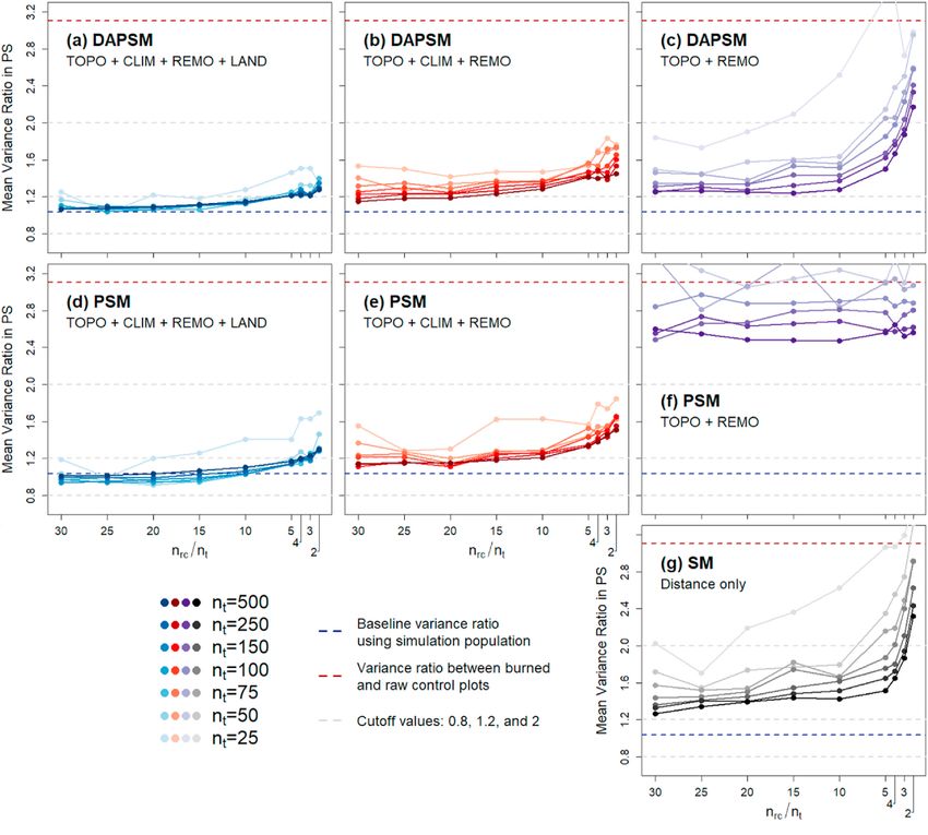
H. Woo et al. Environmental Modelling and Software 144 (2021) 105163
suggested by Papadogeorgou et al. (2019). DAPSM incorporates spatial as the environmental covariates play an important role in distinguishing
distance measures in addition to the estimated propensity scores to ac treated and raw control observations. By implementing matching
count for unobserved covariates. The application of PSM and DAPSM to methods as quasi-experimental approach, causal effects can be esti
ecological data, however, was introduced only recently (e.g., Butsic mated from observational data to inform ecological problems for which
et al., 2017a; Woo et al., 2021), so the performance of these matching experimental settings are impractical.
methods in terms of balance between treated and control groups and
unbiasedness of the estimates under different data availability scenarios 2. Data
is still unknown. Unlike large survey data from health science and
econometrics (e.g., >30,000 treated and >60,000 untreated from 2.1. Forest inventory data
Smeeth et al., 2009; >3000 treated and >100,000 untreated from Huber
et al., 2013), ecological data sets associated with natural disturbances We used national forest inventory data of Washington and Oregon,
are often limited in size due to the scarcity of the natural disturbance USA, from the United States Department of Agriculture Forest Service
events (e.g., wildfire, disease, or insect outbreak) or the cost of data Forest Inventory and Analysis (FIA) program (Smith 2002). Since 2000,
collection over large spatial and temporal scales (Kremens et al., 2010). the FIA program has collected field measurements of forested lands (i.e.,
In matching, availability of data can be identified based on the number at least 10 percent potential cover by live trees) by measuring perma
of treated observations, raw control observations, and environmental nent plots (4047-square meter in size) that represent a spatially
covariates to estimate the propensity scores. Limited data on any of balanced sample of one plot for every 2400 ha (Bechtold and Patterson
these may affect the reliability of the causal effect quantification (Stuart 2005). A plot consists of four circular subplots, and the measurements of
2010). The number of treated observations is directly related to the trees and environmental attributes are made at both plot and subplot
variance of the estimated treatment effect (Brookhart et al., 2006), and level. Ten percent of the plot locations are visited annually, resulting on
the number of raw control observations relative to the treated obser a 10-year remeasurement cycle (Bechtold and Patterson 2005).
vations is associated with the bias in propensity scores (Heinrich et al., Between 2001 and 2016, there were a total of 23,150 inventory plot
2010). The availability of covariates influences the exclusion of impor measurements in Washington and Oregon forests including 7994
tant confounding variables when estimating the propensity scores remeasurements. We classified the plot measurements into burned (i.e.,
(Heckman et al., 1997). Given that matching based on limited data may treated, t) and unburned (i.e., raw control, rc) based on the Monitoring
impose more severe bias on the effect estimation than regression ad Trends in Burn Severity (MTBS, http://www.mtbs.gov/) map. Burned
justments (Stuart 2010), it is critical to understand the performance of plots were identified by spatially overlaying the plot locations on the fire
matching methods under different data availability scenarios and maps. Every FIA plot measurement that fell within the perimeter of a
identify a marginal size of data and covariate set required to implement wildfire that occurred less than five years prior to the measurement was
matching methods. labeled as burned. Meanwhile, plots that had not burned at least ten
This study provides a sensitivity analysis of matching on data years prior to measurement were labeled as unburned. Here we refer to
availability in terms of the balance achieved in propensity score distri the burned measurements as ‘burned plots’ and unburned measurements
butions and of the estimated effect using a case study of wildfire effect as ‘unburned plots’ for simplicity. Thus, unburned plots may have
estimation. Woo et al. (2021) quantified the effect of wildfires on repeated measurements at the same location. To remove dependencies
aboveground live woody forest carbon using DAPSM and PSM based on among burned and unburned plots, previous measurements of burned
an empirical dataset of 23,150 forest inventory plot measurements from plots were excluded from the pool of raw control plots. Similarly, if a
Washington and Oregon, United States of America (USA). Taking plot burned twice, the measurements after the first wildfire were also
advantage of the large number of forest inventory plot measurements excluded to preclude the effect of reburn (Woo et al., 2021). A total of
used in Woo et al. (2021), we performed a Monte Carlo simulation to 611 burned plots and 22,539 unburned plot measurements were used for
generate subsets of the full dataset that contained 611 burned plots (i.e., the analysis. More details on the compilation of the data are available in
treated) and 22,539 unburned plots (i.e., raw control). The propensity Woo et al. (2021).
scores of the burned and unburned plots were estimated based on
sixteen covariates that describe the different environment of plots, with 2.2. Environmental covariates
and without distance adjustment. We examined three scenarios of data
availability: 1) number of burned plots, 2) ratio of unburned plots For each forest inventory plot, we retrieved sixteen environmental
relative to burned plots, and 3) availability of environmental covariates. covariates that are associated with the probability of wildfire occur
For 3), we considered availability of the covariates based on data sources rence. These environmental covariates were grouped into four cate
to define four groups: topography, climate, land cover, and gories: 1) topography (TOPO), 2) climate (CLIM), 3) land cover (LAND),
remote-sensing variables. We first assessed how well the propensity and 4) remotely-sensed variables (REMO) (Table 1; additional details in
score distributions were balanced between the burned and the control Woo et al., 2021).
plots through matching. We then observed how the estimated wildfire Topography and land cover variables of the forest inventory plots
effect changed under the different scenarios. The effects of wildfire were were measured in the field and obtained from the FIA database.
quantified as the difference in live woody carbon mass between the Topography covariates included elevation, slope, and aspect. Elevation
burned and the control plots. We presented the balance achieved and was measured at the center of the plot, and slope and aspect were
effect estimates under DAPSM and PSM to assess the bias and variability measured at subplot level according to the land classification within the
expected within each matching method and data availability scenario. subplot (e.g., forested/non-forested land). We used the values of slope
By providing a sensitivity analysis of DAPSM and PSM based on real- and aspect that accounted for the largest percentage of the forested land
world data, the results of this study suggest practical guidelines of data classification within the subplots. Land cover covariates including land
availability to be considered for wildfire effect quantification and, by ownership, physiographic condition, and proportion of forested area
extension, estimation of other natural disturbance (e.g., Arovaara et al., (Table 1) were measured at subplot level. For the class variables, we
1984) and management effects (e.g., Butsic et al., 2017b). Utilization of used two categories of land ownership (public and private) and three of
national forest inventory data will broaden the opportunity to conduct physiographic class (mesic, xeric, and hydric) (Woo et al., 2021). We
effect analyses over large spatial and temporal scales with spatially assigned the land cover categories that accounted for the largest per
balanced samples of forest conditions. The diagnostics of balance centage within the four subplots.
achievement by matching presented in this study are applicable for Climate covariates consisted of six PRISM-derived variables related
designing future quasi-experiments where the spatial distances as well to precipitation, temperature, vapor pressure, and moisture stress (Daly
2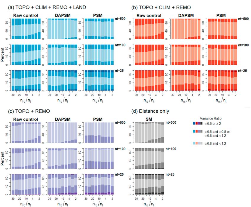
H. Woo et al. Environmental Modelling and Software 144 (2021) 105163
Table 1 3. Matching methods
Descriptions and sources of sixteen environmental variables used for matching
burned and unburned forest inventory plots. 3.1. PSM and DAPSM for assessing wildfire effects on aboveground live
Variable Abbr. Measurement unit/Description woody carbon
Topography (TOPO)
Elevation ELEV Metres Propensity scores in PSM denote the probability of receiving the
Slope SLOPE Degrees treatment conditional on the environmental covariates. The probability
Aspect ASPECT Cosine value, degrees azimuth assigned to each observation – in this study, the forest inventory plot – is
Land cover (LAND)
generally estimated using logistic regression. Distance-adjusted pro
Proportion of forested PROPforest % of plot area with forested condition (at
area least 10 percent potential cover by live pensity scores in DAPSM consider spatial distances between burned and
trees) unburned plot locations in matching. They are a weighted average be
Owner group code OWNGC Categorical: Public, Private tween the propensity scores estimated from environmental covariates
Physiographic class PHYSCL Categorical: Xeric, Mesic, Hydric and the normalized Euclidean distances between plot locations (Papa
Climate (CLIM)
Annual precipitation PRECP ln mm * 100
dogeorgou et al., 2019). Because the spatial distance may take into ac
Mean annual TEMP degrees C * 100 count unobserved covariates that were not included in the covariate set
temperature to estimate the propensity scores, DAPSM should be preferred to PSM or
Coefficient of variation CVPRECP Variation between mean monthly spatial matching (SM) that considers only the distances for matching
in precipitation precipitation of December and July
(Woo et al., 2021).
(wettest and driest months)
Mean temperature TEMPDIF degrees C * 100, difference between mean The quantification of wildfire effects on aboveground live woody
difference August maximum temperature and mean carbon using the matching methods followed three steps: First, we
December minimum temperature estimated propensity scores of burned and unburned plots using logistic
Mean summer vapor SVPD hPa regression with the sixteen environmental covariates. Then, we esti
pressure deficit
mated the distance-adjusted propensity scores as a linear combination of
Growing season GSMS degrees C/ln mm, ratio of temperature to
moisture stress precipitation from May–September the propensity scores and spatial distances between pairs of burned and
Remotely-sensed data (REMO) unburned plots. We used a weight of 0.5 to equally emphasize the
Normalized difference NDVI observed environmental covariates and the spatial distance, given an
in vegetation index
earlier study that found other weights (i.e., 0.25, 0.5, and 0.75) did not
Tasseled cap brightness TC1
Tasseled cap greenness TC2 result in any difference in the effect estimation (Woo et al., 2021).
Tasseled cap wetness TC3 Finally, we matched the burned plots and unburned plots using PSM and
DAPSM to obtain a set of control plots that share similar covariates and
geographical locations. We employed matching without replacement
et al., 2008). The climate covariates were derived from thirty-year with a greedy algorithm (Austin 2011) that sequentially finds the
normal data (1981–2010) with 30-m resolution. The remote-sensing smallest difference in the distance-adjusted propensity scores between
data included four spectral and vegetation indices including the the burned and the unburned plots. This algorithm is the most
normalized difference vegetation index (NDVI), and tasseled cap commonly used in propensity score matching implementation (Austin
brightness, greenness, and wetness in the middle of growing season, all and Cafri 2020). The matched unburned plots were identified as control
derived from annual Landsat satellite images with 30-m resolution. plots. The estimates of the wildfire effects were then quantified as the
Unburned plots were associated with the remotely-sensed variables in difference in aboveground live woody carbon mass between the burned
the year that the plot was measured, and burned plots were associated and control plots.
with the variables measured in a year before the wildfire to account for
stand characteristics that may be related to the risk of burning. To assign 3.2. Sensitivity analysis of DAPSM under different data availability
the climate and remotely-sensed covariates to each of the plot mea scenarios
surements the values of 9 pixels around the plot center location were
averaged. The climate and remotely-sensed metrics were obtained from We ran Monte Carlo simulations to perform a sensitivity analysis on
the Landscape Ecology, Modeling, Mapping, and Analysis (LEMMA) the balance of propensity score distributions as well as effect estimates
team (https://lemma.forestry.oregonstate.edu/). when reducing the number of treated and raw control observations and
covariate sets. We created random subsets of forest inventory plot data
2.3. Aboveground live woody carbon from the full data consisting of 611 burned plots (Nt =611) and 22,539
unburned plots (Nrc =22,539). The full data was set as our reference
We obtained aboveground live woody carbon mass per plot (Mg population for the Monte Carlo simulations (i.e., simulation population),
ha− 1) for both burned and unburned plots, based on all live trees over and the propensity scores estimated based on all available environ
2.54 cm diameter at breast height (DBH) measured within the forest mental covariates using the simulation population were considered to be
inventory plot by the FIA protocol (Bechtold and Patterson 2005). the true propensity scores in our simulation. Because the number of
Aboveground woody biomass including stem, bark, and live branches possible combinations of all covariates is very large, we grouped the
was estimated by the Pacific Northwest Research Station, USDA Forest environmental covariates sharing similar attributes and sources as
Service (Woodall et al., 2012). We converted the aboveground live stated in Section 2.2 based on the idea that the attainability of variables
woody biomass into carbon mass using a carbon ratio multiplier of 0.5 is dependent on the accessibility to the data source. For example, TOPO
(IPCC 2006). The obtained carbon mass was summarized as per ha including elevation, slope, and aspect are easily available for researchers
values (Mg ha− 1) for each plot, and used as the outcome variable in through open sources such as digital elevation models (DEM) or
propensity score matching to assess the effect of wildfires. The estimated geographical information systems (GIS) for most regions (Bungartz
wildfire effect is the difference in the outcome variable between burned et al., 2018). The order of accessibility to the four groups of covariates in
and unburned plots. our study was identified as TOPO-CLIM-REMO-LAND from the least to
the most costly to obtain. We considered four scenarios of environ
mental covariate sets for propensity score estimation: 1) full set of
covariates with all four groups TOPO + CLIM + REMO + LAND, 2)
TOPO + CLIM + REMO, 3) TOPO + CLIM, and 4) TOPO + REMO
3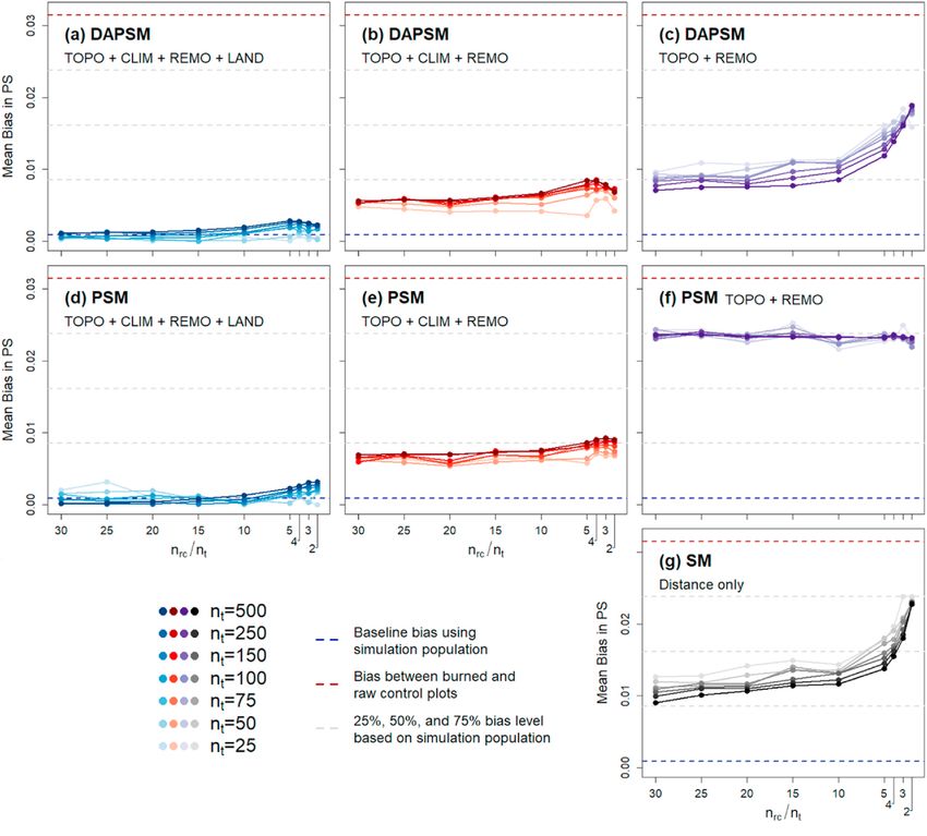
H. Woo et al.                                                                                                             Environmental Modelling and Software 144 (2021) 105163

Table 2                                                                                         of the covariates on the estimated propensity scores. If the matching was
Simulated data availability scenarios and their values and conditions for DAPSM                 successful and the control group is similar to the treated group, the
and PSM. SM simulated nt and nrc /nt only.                                                      means of difference and the variance ratios of the propensity scores
  Simulated scenarios          Values/Conditions                                                should be close to zero and one, respectively. Ratio of variance between
  Number of burned plots       500, 250, 150, 100, 75, 50, 25
                                                                                                0.8 and 1.2 is considered adequate, while values below 0.5 or over 2 are
   (nt )                                                                                        too extreme (Rubin 2001). For the ratio of the variances of the residuals
  Matching ratio (nrc / nt )   30, 25, 20, 15, 10, 5, 4, 3, 2                                   of the covariates, we computed the percentage of covariates that are
  Covariate set                1) TOPO + CLIM + REMO + LAND– full set of                        within each of the variance ratio ranges (i.e., ≤0.8 and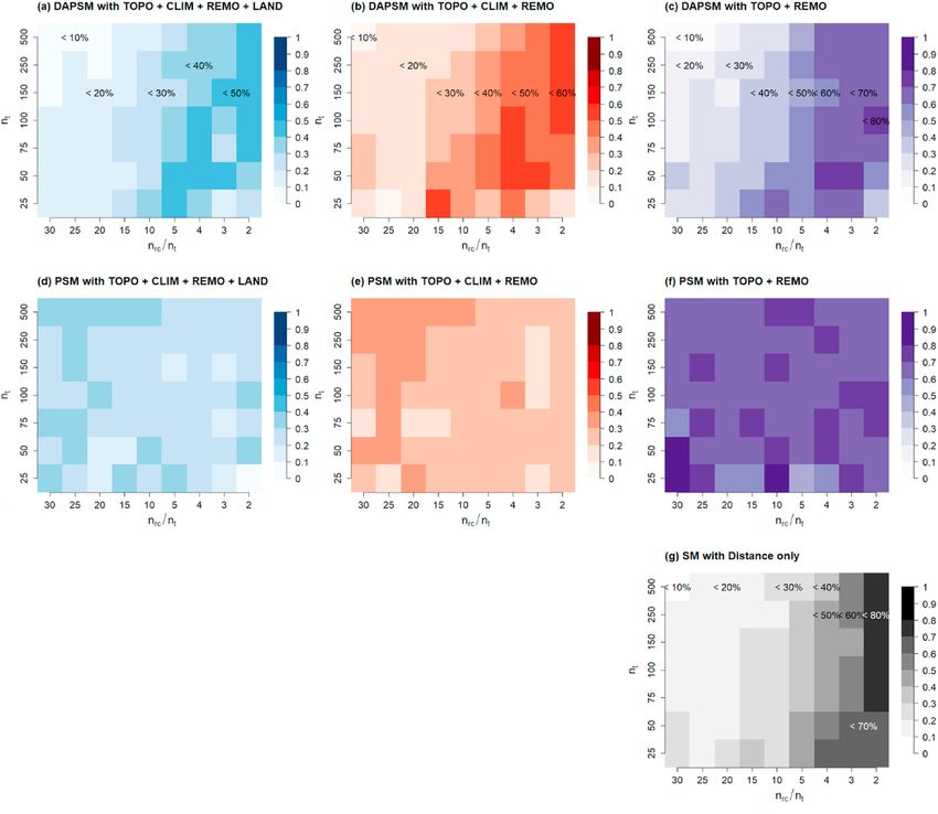
H. Woo et al. Environmental Modelling and Software 144 (2021) 105163
4. Results matching process did not result in large differences in mean bias in
propensity scores as long as CLIM variables were included in the co
4.1. Balance in propensity scores under different data availability variate set (Fig. 1a vs. 1d and Fig. 1b vs. 1e). Without CLIM variables,
scenarios PSM produced much larger bias than DAPSM regardless of nrc /nt
(Fig. 1f). Without any environmental covariates included in the
4.1.1. Smaller mean bias in propensity scores under larger nt and covariate matching process (i.e., SM with distance only; Fig. 1e), the mean bias
set with CLIM showed a similar pattern to DAPSM without CLIM (Fig. 1c): small in
The three scenarios of data availability in matching (i.e., nt , nrc / nt , crease in mean bias on average and a sharp increase in mean bias when
and covariate set) jointly affected the mean bias in propensity scores nrc /nt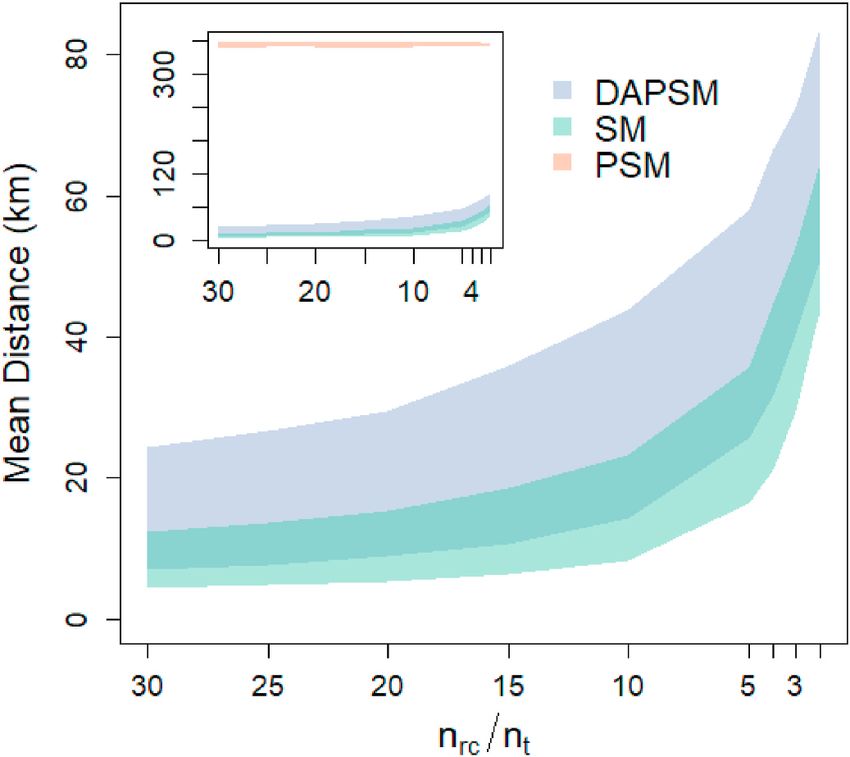
H. Woo et al. Environmental Modelling and Software 144 (2021) 105163
Fig. 2. Mean variance ratio in propensity scores (PS) between burned and control plots under different combinations of number of burned plots (nt ), unburned plots
to burned plots (nrc /nt ), and covariate set, matched based on (a)–(c) DAPSM, (d)–(f) PSM, or (g) SM. The cutoff values of variance ratio from Rubin (2001): values
between 0.8 and 1.2 are considered to be adequate, while values > 2 are extreme. Values outside the range of the graphs are available in Fig. S2 in the supple
mentary materials.
distributions of propensity scores between burned and control plots. were observed for the matched plots, regardless of nrc /nt (Fig. 3a–d). nt
PSM produced slightly smaller variance ratios than DAPSM did when = 25 barely reduced the variance ratio for any nrc /nt through matching.
CLIM was included in the covariate set (Fig. 2a vs. 2d, Fig. 2b vs. 2e). When climate variables (CLIM) were included in the covariate set, the
PSM without CLIM, however, did not reduce the variance in propensity distribution of variance ratios obtained through both DAPSM and PSM
scores between burned and unburned plots (red lines in Fig. 2f). Once did not differ much among the covariate sets (Fig. 3a–c). TOPO and
distance was included in the matching process, however, the variance REMO variables, however, showed little initial imbalance in the vari
ratio substantially dropped, especially for large nt (≥100) and nrc / nt ance ratio of residuals between burned and raw control plots (Fig. 3d)
(≥15) values even if no other covariates were included (Fig. 2g). compared to other covariate sets. In that case, PSM introduced more
severe imbalance in variance ratio than the raw controls (Fig. 3d).
4.1.3. Smaller variance ratio of the residuals of the covariates under
DAPSM 4.1.4. DAPSM balances some covariates that were not included in
Comparing raw control to controls obtained through DAPSM and propensity score model
PSM, the improvement in the variance ratio of residuals of individual The average ASMD computed for each covariate showed major dif
covariates through matching was obvious in all covariate sets, showing ferences between DAPSM and PSM under the same covariate set
increase in the percentages of variance ratio between 0.8 and 1.2 (Table 4, Fig. S4). Comparing the raw controls of unburned plots to the
(Fig. 3a–d). DAPSM exhibited larger percentages of variance ratio be burned plots (i.e., unmatched), 11 out of 16 covariates were imbalanced
tween 0.8 and 1.2 than PSM did, indicating the method was more (i.e., ASMD > 0.2). Matching based on the full covariate set achieved
effective achieving balance in terms of individual covariates. SM based balance in all covariates under both DAPSM and PSM. When the co
on distance only was also more balance in individual covariates than variate sets were reduced, PSM resulted in imbalance in the omitted
PSM, especially when nrc /nt >10 (Fig. 3d). covariates (e.g., PHYSCL, TEMP, TEMPDF, SVPD, and GSMS under PSM
As nt decreased, increasingly extreme variance ratios of the residuals with TOPO + REMO; Table 4). On the other hand, DAPSM accomplished
6
H. Woo et al.                                                                                                      Environmental Modelling and Software 144 (2021) 105163

Fig. 3. Percentages of the number of covariates of which residual variance ratio falls within each range under the covariate set (a) TOPO + CLIM + REMO + LAND,
(b) TOPO + CLIM + REMO, and (c) TOPO + REMO using DAPSM and PSM and (d) SM. Darker colours present more extreme variance ratios: < 0.5 or ≥2 (extreme),
≥0.5 and 0.2 and ≤0.4 indicates moderate imbalance, and ASMD >0.4 indicates severe imbalance.

                                                                                   7
H. Woo et al. Environmental Modelling and Software 144 (2021) 105163
balance in climate variables even though the CLIM covariates were nrc /nt values under DAPSM deviated on average by 25–30% from the
excluded in the propensity score estimation. SM generally achieved baseline estimate when the covariate set included CLIM variables
balance in most of the covariates except for SLOPE and PHYSCL despite (Fig. 4a and b), whereas the average deviation was 43% for the covariate
the withdrawal of all covariates in the matching process. sets without CLIM variables (Fig. 4c). nt less than 100 tended to show
large variability in the wildfire effect estimates, resulting in positive
effect estimates for a few subsets.
4.2. Performance of wildfire effect estimates under different data
The bias of the effect estimates tended to increase with decreases in
availability scenarios
nt and nrc /nt under DAPSM (Fig. 4a–c), while the bias of PSM-derived
estimates was mostly dependent on covariate sets only, not on nt or nrc /
Again, the three data availability scenarios nt , nrc / nt , and covariate
nt (Fig. 4d–f). The matrix plots (Fig. 5) suggested that the bias was
set affected the bias and variance of wildfire effect estimates collec
susceptible to small nrc /nt than small nt . When CLIM was included in the
tively. Under DAPSM, the number of burned plots in the simulation
covariate set, controls from DAPSM with nt = 100 and nrc /nt = 20 were
subsets (nt ) was related to the bias of the estimates of average wildfire
found to show 20% bias compared to the simulation population (Fig. 5a
effect, whereas the ratio of unburned to burned plots (nrc / nt ) influenced
and c). For small numbers of nt and nrc /nt (e.g., ntH. Woo et al. Environmental Modelling and Software 144 (2021) 105163 Fig. 5. Matrix plot of percent bias in the wildfire effect estimates under different combinations of nt , nrc /nt , and covariate sets. For example, the combination of nt = 150 and nrc /nt = 15 exhibited less than 20% of bias compared to the baseline estimate under (a) TOPO + CLIM + REMO + LAND,
H. Woo et al. Environmental Modelling and Software 144 (2021) 105163
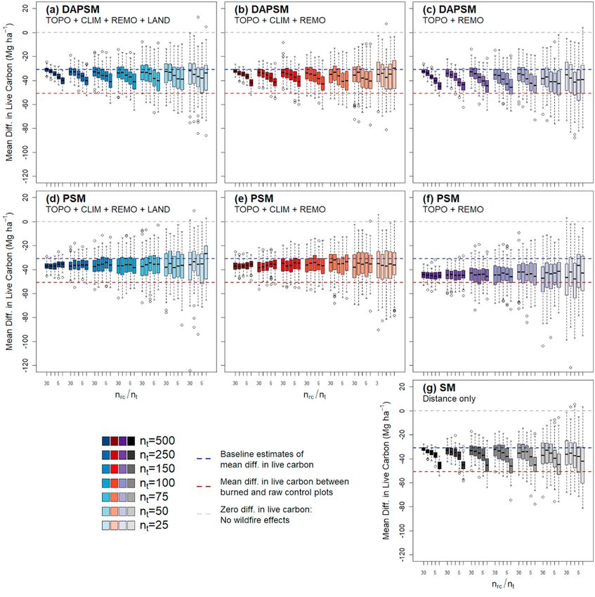
5.2. Sample size suggestion based on the effect estimates using DAPSM
and forest inventory data
The effect of spatial distance in the performance of the matching was
also evident from the estimated effect of wildfire, defined as the dif
ference in live carbon between burned and control plots. DAPSM was
superior to PSM showing less bias, most likely because the spatial dis
tance accounted for additional information from unobserved covariates.
These results agree with a recent clinical study that shows that spatial
propensity score matching outperformed non-spatial matching (Davis
et al., 2021). However, our study further showed that including the
distance measure was less effective or counterproductive when the
sample size was very small and the distance between possible matches
too large. Then, the spatial distance provided no additional information,
resulting in an even larger bias in the estimates. While the critical
sample size may be scale dependent, based on the results of simulated
estimates, we suggest a sample size of at least nt = 100 and nrc /nt = 10 as
the threshold to apply DAPSM over Washington and Oregon. This
threshold of number of treated and raw control observations can serve as
a practical guideline when implementing DAPSM for further research
using forest inventory at regional scales. Further research may not be
limited to wildfire effects on carbon mass but on various outcomes of
Fig. 6. Mean distance between matched pairs of burned and control plots under interest that are closely related with climate variables, such as vegeta
DAPSM, SM, and PSM across nrc /nt . tion structure (Duguy et al., 2013), biodiversity (Gill et al., 2013), or
land use (Duguy et al., 2012).
variables. Even SM, based solely on spatial distance, outperformed PSM The bias in the estimates of wildfire effects observed from our study
without CLIM variables. The results emphasize the importance of was generally larger than the results from Pirracchio et al. (2012) who
incorporating spatial measures to account for both observed and unob obtained less than 10% of relative bias when decreasing the sample size
served confounding factors (Woo et al., 2021; Papadogeorgou et al., from 1000 to 40. The relative bias from Pirracchio et al. (2012) was
2019). obtained from Monte Carlo simulations using an artificial dataset for
However, incorporating spatial proximity was no longer effective as which the data generation process was known. It is common to use an
the observations became sparser over the study area. The bias and artificial dataset for sensitivity analyses of PSM (e.g., Coffman et al.,
variance ratio in propensity scores were remarkably large under sample 2020; Rubin and Thomas 1996) based on the true propensity score
sizes nt around 150 or less and nrc /ntH. Woo et al. Environmental Modelling and Software 144 (2021) 105163
quasi-experimental methods will provide opportunities of continuous Appendix A. Supplementary data
causal effect analysis for ecological data.
Supplementary data to this article can be found online at https://doi.
6. Conclusion org/10.1016/j.envsoft.2021.105163.
This study presented a sensitivity analysis of distance-adjusted pro References
pensity score matching (DAPSM) in relation to data availability. We
examined three data availability scenarios in matching: number of Abadie, A., Imbens, G.W., 2006. Large sample properties of matching estimators for
average treatment effects. Econometrica 74, 235–267.
available burned plots, number of unburned plots relative to burned Arovaara, H., Hari, P., Kuusela, K., 1984. Possible Effect of Changes in Atmospheric
plots, and environmental covariate set to estimate the propensity scores Composition and Acid Rain on Tree Growth. An Analysis Based on the Results of
for the quantification of wildfire effects using national forest inventory Finnish National Forest Inventories. Finnish Forest Research Institute.
Austin, P.C., 2009. Balance diagnostics for comparing the distribution of baseline
plot measurements in Washington and Oregon. We conducted Monte covariates between treatment groups in propensity-score matched samples. Stat.
Carlo simulations of random subsets of burned and unburned plots to Med. 28, 3083–3107.
quantify the wildfire effects under different covariate sets. For each Austin, P.C., 2011. An introduction to propensity score methods for reducing the effects
of confounding in observational studies. Multivariate Behav. Res. 46, 399–424.
simulation, performance of DAPSM was evaluated as the bias and Austin, P.C., Cafri, G., 2020. Variance estimation when using propensity-score matching
variance ratio of propensity scores as well as the bias and variability of with replacement with survival or time-to-event outcomes. Stat. Med. 39,
the estimates of wildfire effect. We studied the influence of distance 1623–1640.
Bechtold, W.A., Patterson, P.L., 2005. The enhanced forest inventory and analysis
measure in matching by comparing the performance of DAPSM to that of
program-national sampling design and estimation procedures. Gen. Tech. Rep. SRS-
matching without distance adjustment. 80. Asheville, NC US Dep. Agric. For. Serv. South. Res. Station. 85, 80.
We found that the three data availability scenarios interacted to Bennett, N.D., Croke, B.F.W., Guariso, G., Guillaume, J.H.A., Hamilton, S.H.,
affect the performance of matching. Among the three scenarios, whether Jakeman, A.J., Marsili-Libelli, S., Newham, L.T.H., Norton, J.P., Perrin, C., 2013.
Characterising performance of environmental models. Environ. Model. Softw. 40,
the covariate set included climate variables or not dominated the degree 1–20.
of balance in propensity score distributions between burned and control Brookhart, M.A., Schneeweiss, S., Rothman, K.J., Glynn, R.J., Avorn, J., Stürmer, T.,
plots. Climate variables turned out to be the key covariates to analyze 2006. Variable selection for propensity score models. Am. J. Epidemiol. 163,
1149–1156.
the wildfire effect on forest carbon mass. The sample size, especially the Bungartz, H.-J., Kranzlmüller, D., Weinberg, V., Weismüller, J., Wohlgemuth, V., 2018.
number of unburned plots relative to the burned plots, was closely Advances and New Trends in Environmental Informatics. Springer.
related with the distance between the matched pairs. Large distance Butsic, V., Lewis, D.J., Radeloff, V.C., Baumann, M., Kuemmerle, T., 2017a. Quasi-
experimental methods enable stronger inferences from observational data in
among the plots due to sparseness of observations over the region ecology. Basic Appl. Ecol. 19, 1–10.
resulted in severe bias and variability in the effect estimates because the Butsic, V., Munteanu, C., Griffiths, P., Knorn, J., Radeloff, V.C., Lieskovský, J.,
key covariates were not accounted for by the distance measure. Mueller, D., Kuemmerle, T., 2017b. The effect of protected areas on forest
disturbance in the Carpathian Mountains 1985–2010. Conserv. Biol. 31, 570–580.
Based on our results, the importance of key covariates and the in Campbell, D.T., Stanley, J.C., 2015. Experimental and Quasi-Experimental Designs for
clusion of the spatial measure were emphasized for applying propensity Research. Ravenio Books, Boston, MA.
score matching methods to account for both observed and unobserved Carlson, C.H., Dobrowski, S.Z., Safford, H.D., 2012. Variation in tree mortality and
regeneration affect forest carbon recovery following fuel treatments and wildfire in
confounding variables. We also suggest a marginal sample size with at
the Lake Tahoe Basin, California, USA. Carbon Balance Manag 7, 1–17.
least a hundred treated observations and a tenfold larger number of raw Coffman, D.L., Zhou, J., Cai, X., 2020. Comparison of methods for handling covariate
controls to implement DAPSM over Washington and Oregon to achieve missingness in propensity score estimation with a binary exposure. BMC Med. Res.
balance in propensity score distributions and low bias in effect esti Methodol. 20, 168. https://doi.org/10.1186/s12874-020-01053-4.
Cohen, J., 2013. Statistical Power Analysis for the Behavioral Sciences. Academic press,
mates. Future studies implementing matching approaches for effect New York.
analyses using forest inventory plot data will find this research useful to Daly, C., Halbleib, M., Smith, J.I., Gibson, W.P., Doggett, M.K., Taylor, G.H., Curtis, J.,
determine the sample size and covariate set in relation with spatial Pasteris, P.P., 2008. Physiographically sensitive mapping of climatological
temperature and precipitation across the conterminous United States. Int. J.
distances among the observations. National forest inventory data facil Climatol. a J. R. Meteorol. Soc. 28, 2031–2064.
itate monitoring and the assessment of comprehensive forest resources Davis, M.L., Neelon, B., Nietert, P.J., Burgette, L.F., Hunt, K.J., Lawson, A.B., Egede, L.E.,
over large spatial and temporal scales. Utilization of DAPSM with forest 2021. Propensity score matching for multilevel spatial data: accounting for
geographic confounding in health disparity studies. Int. J. Health Geogr. 20, 1–12.
inventory data enables rigorous research on effect analysis not limited to https://doi.org/10.1186/s12942-021-00265-1.
wildfires but applicable to other disturbances and ecological processes Di Cecco, G.J., Gouhier, T.C., 2018. Increased spatial and temporal autocorrelation of
where a randomized experiment is infeasible. temperature under climate change. Sci. Rep. 8, 1–9.
Dixon, R.K., Solomon, A.M., Brown, S., Houghton, R.A., Trexier, M.C., Wisniewski, J.,
1994. Carbon pools and flux of global forest ecosystems. Science 263, 185–190.
Declaration of competing interest Dray, S., Legendre, P., Peres-Neto, P.R., 2006. Spatial modelling: a comprehensive
framework for principal coordinate analysis of neighbour matrices (PCNM). Ecol.
Modell. 196, 483–493. https://doi.org/10.1016/j.ecolmodel.2006.02.015.
The authors declare that they have no known competing financial
Duguy, B., Alloza, J.A., Baeza, M.J., De La Riva, J., Echeverría, M., Ibarra, P., Llovet, J.,
interests or personal relationships that could have appeared to influence Cabello, F.P., Rovira, P., Vallejo, R.V., 2012. Modelling the ecological vulnerability
the work reported in this paper. to forest fires in mediterranean ecosystems using geographic information
technologies. Environ. Manage. 50, 1012–1026. https://doi.org/10.1007/s00267-
012-9933-3.
Acknowledgements Duguy, B., Paula, S., Pausas, J.G., Alloza, J.A., Gimeno, T., Vallejo, R.V., 2013. In:
Navarra, A., Tubiana, L. (Eds.), Effects of Climate and Extreme Events on Wildfire
This study was supported partly by 4-year doctoral fellowship from Regime and Their Ecological Impacts BT - Regional Assessment of Climate Change in
the Mediterranean: Volume 2: Agriculture, Forests and Ecosystem Services and
the Faculty of Forestry provided by the University of British Columbia, People. Springer Netherlands, Dordrecht, pp. 101–134. https://doi.org/10.1007/
Canada. We thank Matthew Gregory from the Landscape Ecology, 978-94-007-5772-1_6.
Modeling, Mapping, and Analysis (LEMMA) team for his assistance with Eskelson, B.N.I., Monleon, V.J., Fried, J.S., 2016. A 6 year longitudinal study of post-fire
woody carbon dynamics in California’s forests. Can. J. For. Res. 46, 610–620.
the PRISM and Landsat data retrieval and compilation. We also thank https://doi.org/10.1139/cjfr-2015-0375.
the many individuals involved in the design, field data collection, Gill, A.M., Stephens, S.L., Cary, G.J., 2013. The worldwide “wildfire” problem. Ecol.
quality assurance, and processing of the U.S. Forest Service Forest In Appl. 23, 438–454.
Greenstone, M., Gayer, T., 2009. Quasi-experimental and experimental approaches to
ventory and Analysis Program. environmental economics. J. Environ. Econ. Manage. 57, 21–44.
Heckman, J.J., Ichimura, H., Todd, P.E., 1997. Matching as an econometric evaluation
estimator: evidence from evaluating a job training programme. Rev. Econ. Stud. 64,
605–654.
11H. Woo et al. Environmental Modelling and Software 144 (2021) 105163
Heinrich, C., Maffioli, A., Vazquez, G., 2010. A Primer for Applying Propensity-Score Pianosi, F., Beven, K., Freer, J., Hall, J.W., Rougier, J., Stephenson, D.B., Wagener, T.,
Matching. Inter-American Dev. Bank. 2016. Sensitivity analysis of environmental models: a systematic review with
Huber, M., Lechner, M., Wunsch, C., 2013. The performance of estimators based on the practical workflow. Environ. Model. Softw. 79, 214–232.
propensity score. J. Econom. 175, 1–21. Pirracchio, R., Resche-Rigon, M., Chevret, S., 2012. Evaluation of the Propensity score
IPCC, 2006. IPCC guidelines for national greenhouse gas inventories. In: Agriculture, methods for estimating marginal odds ratios in case of small sample size. BMC Med.
Forestry and Other Land Use, ume 4. Institute for Global Environmental Strategies Res. Methodol. 12, 70. https://doi.org/10.1186/1471-2288-12-70.
(IGES). Rosenbaum, P.R., Rubin, D.B., 1983. The central role of the propensity score in
Jain, T.B., Fried, J.S., 2010. Field instructions for the annual inventory of California, observational studies for causal effects. Biometrika 70, 41–55.
Oregon, and Washington 2010: supplement for: fire effects and recovery study. US Rubin, D.B., 2001. Using propensity scores to help design observational studies:
Dep. Agric. For. Serv. Pacific Northwest Res. Station. For. Invent. Anal. Resour. application to the tobacco litigation. Health Serv. Outcome Res. Methodol. 2,
Monit. Assess. Program. 30. 169–188.
Keith, H., Lindenmayer, D.B., Mackey, B.G., Blair, D., Carter, L., McBurney, L., Okada, S., Rubin, D.B., Thomas, N., 1996. Matching using estimated propensity scores: relating
Konishi-Nagano, T., 2014. Accounting for biomass carbon stock change due to theory to practice. Biometrics 52, 249–264. https://doi.org/10.2307/2533160.
wildfire in temperate forest landscapes in Australia. PloS One 9, e107126. https:// Rudolph, K.E., Stuart, E.A., 2018. Using sensitivity analyses for unobserved confounding
doi.org/10.1371/journal.pone.0107126. to address covariate measurement error in propensity score methods. Am. J.
Kremens, R.L., Smith, A.M.S., Dickinson, M.B., 2010. Fire metrology: current and future Epidemiol. 187, 604–613. https://doi.org/10.1093/aje/kwx248.
directions in physics-based measurements. Fire Ecol 6, 13–35. Smeeth, L., Douglas, I., Hall, A.J., Hubbard, R., Evans, S., 2009. Effect of statins on a
Larsen, A.E., Meng, K., Kendall, B.E., 2019. Causal analysis in control–impact ecological wide range of health outcomes: a cohort study validated by comparison with
studies with observational data. Methods Ecol. Evol. 10, 924–934. https://doi.org/ randomized trials. Br. J. Clin. Pharmacol. 67, 99–109.
10.1111/2041-210X.13190. Smith, W.B., 2002. Forest inventory and analysis: a national inventory and monitoring
Lechner, M., Wunsch, C., 2013. Sensitivity of matching-based program evaluations to the program. Environ. Pollut. 116, S233–S242.
availability of control variables. Labour Econ 21, 111–121. Stegen, J.C., Swenson, N.G., Enquist, B.J., White, E.P., Phillips, O.L., Jørgensen, P.M.,
Liu, S., Bond-Lamberty, B., Hicke, J.A., Vargas, R., Zhao, S., Chen, J., Edburg, S.L., Weiser, M.D., Monteagudo Mendoza, A., Núñez Vargas, P., 2011. Variation in above-
Hu, Y., Liu, J., McGuire, A.D., Xiao, J., Keane, R., Yuan, W., Tang, J., Luo, Y., ground forest biomass across broad climatic gradients. Global Ecol. Biogeogr. 20,
Potter, C., Oeding, J., 2011. Simulating the impacts of disturbances on forest carbon 744–754.
cycling in North America: processes, data, models, and challenges. J. Geophys. Res. Stuart, E.A., 2010. Matching methods for causal inference: a review and a look forward.
116, G00K08. https://doi.org/10.1029/2010JG001585. Stat. Sci. 25, 1–21. https://doi.org/10.1214/09-STS313.
McCaffrey, D.F., Griffin, B.A., Almirall, D., Slaughter, M.E., Ramchand, R., Burgette, L.F., Stuart, E.A., Rubin, D.B., 2004. Matching Methods for Causal Inference: Designing
2013. A tutorial on propensity score estimation for multiple treatments using Observational Studies. Harvard Univ. Dep. Stat. mimeo.
generalized boosted models. Stat. Med. 32, 3388–3414. Turner, M.G., O’Neill, R.V., Gardner, R.H., Milne, B.T., 1989. Effects of changing spatial
McKenzie, D., Gedalof, Z., Peterson, D.L., Mote, P., 2004. Climatic change, wildfire, and scale on the analysis of landscape pattern. Landsc. Ecol. 3, 153–162.
conservation. Conserv. Biol. 18, 890–902. Wang, W.J., He, H.S., Spetich, M.A., Shifley, S.R., Thompson, F.R., Dijak, W.D.,
Nolte, C., Agrawal, A., Silvius, K.M., Soares-Filho, B.S., 2013. Governance regime and Wang, Q., 2014. A framework for evaluating forest landscape model predictions
location influence avoided deforestation success of protected areas in the Brazilian using empirical data and knowledge. Environ. Model. Softw. 62, 230–239.
Amazon. Proc. Natl. Acad. Sci. Unit. States Am. 110, 4956–4961. Weisberg, P.J., Swanson, F.J., 2003. Regional synchroneity in fire regimes of western
Nolte, C., Gobbi, B., de Waroux, Y., le, P., Piquer-Rodríguez, M., Butsic, V., Lambin, E.F., Oregon and Washington, USA. For. Ecol. Manage. 172, 17–28.
2017. Decentralized land use zoning reduces large-scale deforestation in a major Woo, H., Eskelson, B.N.I., Monleon, V.J., 2021. Matching methods to quantify wildfire
agricultural frontier. Ecol. Econ. 136, 30–40. effects on forest carbon mass in the U.S. Pacific Northwest. Ecol. Appl. 31, e02283.
Papadogeorgou, G., Choirat, C., Zigler, C.M., 2019. Adjusting for unmeasured spatial Woodall, C.W., Perry, C.H., Westfall, J.A., 2012. An empirical assessment of forest floor
confounding with distance adjusted propensity score matching. Biostatistics 20, carbon stock components across the United States. For. Ecol. Manage. 269, 1–9.
256–272.
12You can also read