A note on precision-preserving compression of scientific data - GMD
←
→
Page content transcription
If your browser does not render page correctly, please read the page content below
Geosci. Model Dev., 14, 377–389, 2021
https://doi.org/10.5194/gmd-14-377-2021
© Author(s) 2021. This work is distributed under
the Creative Commons Attribution 4.0 License.

A note on precision-preserving compression of scientific data
Rostislav Kouznetsov1,2
1 Finnish   Meteorological Institute, Helsinki, Finland
2 Obukhov    Institute for Atmospheric Physics, Moscow, Russia

Correspondence: Rostislav Kouznetsov (rostislav.kouznetsov@fmi.fi)

Received: 14 July 2020 – Discussion started: 30 July 2020
Revised: 17 November 2020 – Accepted: 4 December 2020 – Published: 22 January 2021

Abstract. Lossy compression of scientific data arrays is a       1   Introduction
powerful tool to save network bandwidth and storage space.
Properly applied lossy compression can reduce the size of
a dataset by orders of magnitude while keeping all essential     Resolutions and the level of details of processes simulated
information, whereas a wrong choice of lossy compression         with geoscientific models increase together with the increase
parameters leads to the loss of valuable data. An important      in computing power available. A corresponding increase in
class of lossy compression methods is so-called precision-       the size of datasets needed to drive the models and the
preserving compression, which guarantees that a certain pre-     datasets produced by the models makes the problem of trans-
cision of each number will be kept. The paper considers sta-     ferring and archiving the data more and more acute.
tistical properties of several precision-preserving compres-        The data are usually produced and stored as floating-point
sion methods implemented in NetCDF Operators (NCO), a            numbers implemented in most of computer systems accord-
popular tool for handling and transformation of numerical        ing to the IEEE 754-1985 standard (ANSI/IEEE, 1985). The
data in NetCDF format. We compare artifacts resulting from       standard offers two formats: single precision and double pre-
the use of precision-preserving compression of floating-point    cision. The data in these formats have precisions of approx-
data arrays. In particular, we show that a popular Bit Groom-    imately 7 and 16 significant decimal figures and occupy 32
ing algorithm (default in NCO until recently) has subopti-       and 64 bits per value in a memory or on a disk.
mal accuracy and produces substantial artifacts in multipoint       The problem of storing and transferring the data is nor-
statistics. We suggest a simple implementation of two algo-      mally addressed in three directions: increase in storage ca-
rithms that are free from these artifacts and have double the    pacities and network bandwidth, reduction in the number of
precision. One of them can be used to rectify the data already   stored or transferred values by careful selection of required
processed with Bit Grooming.                                     variables and a wise choice of the archiving policies, and the
   We compare precision trimming for relative and absolute       application of various data compression techniques. We will
precision to a popular linear packing (LP) method and find       focus on the latter.
out that LP has no advantage over precision trimming at a           Lossless compression algorithms map a data array to a
given maximum absolute error. We give examples when LP           smaller size in a way that the original data can be restored
leads to an unconstrained error in the integral characteristic   exactly. The algorithms are efficient for datasets of low in-
of a field or leads to unphysical values.                        formation entropy rate, e.g., those that have a lot of repeating
   We analyze compression efficiency as a function of tar-       patterns.
get precision for two synthetic datasets and discuss precision      Many scientific datasets have only a few (or even a few
needed in several atmospheric fields.                            tens of) percent accuracy and thus require much less than
   Mantissa rounding has been contributed to NCO main-           seven decimals to represent a value. When represented with
stream as a replacement for Bit Grooming. The Appendix           standard formats, such datasets have seemingly random num-
contains code samples implementing precision trimming in         bers at less significant places, i.e., have high information en-
Python3 and Fortran 95.                                          tropy. As a result, the application of lossless compression al-
                                                                 gorithms to such datasets does not lead to a substantial reduc-

Published by Copernicus Publications on behalf of the European Geosciences Union.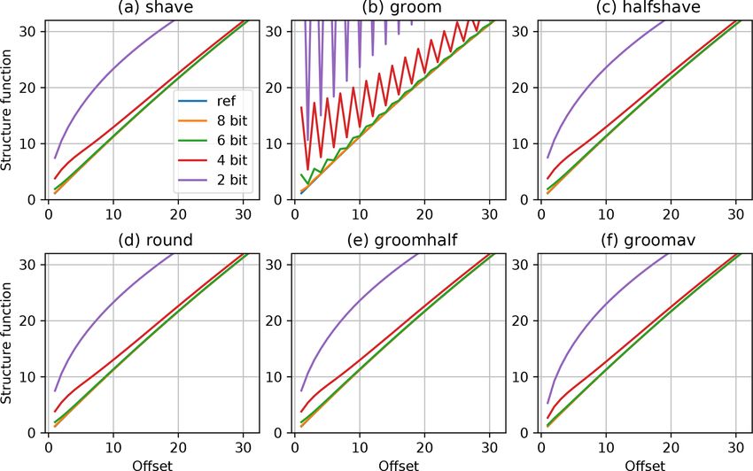
378                                                                      R. Kouznetsov: On precision-preserving compression

tion in the dataset size. Transformations of a data array re-         While comparing spatial structure functions of strato-
ducing its information entropy while introducing acceptable        spheric ozone mixing ratio from satellite retrievals to those
distortions pose the basis for lossy compression algorithms.       obtained from the Silam chemistry-transport model (http:
A transformation can make the array smaller or can facilitate      //silam.fmi.fi, last access: 18 January 2021) and compressed
the performance of subsequent lossless compression. Note           with NCO, we spotted a substantial distortion introduced
that the meaning of “acceptable distortion” depends on the         by Bit Grooming into the structure function of the modeled
data and/or the intended application.                              fields. In the current note we investigate the cause of this dis-
   An often used method of lossy compression is linear pack-       tortion. We consider several precision-trimming algorithms
ing, when the original floating-point data are mapped to a         and the inaccuracies they introduce. We suggest an imple-
shorter-length integer data by a linear transformation. The        mentation of mantissa rounding that provides double the ac-
method, introduced in GRIB (GRidded Binary) format ap-             curacy of the data representation as Bit Grooming with the
proved back in 1985 by the World Meteorological Organi-            same number of data bits and does not introduce major arti-
zation and intended for use for gridded weather data (Stack-       facts in two-point statistics. In addition, we suggest a method
pole, 1994), is still in use in subsequent standards. A simi-      of recovering the bit-groomed data.
lar technique has been applied for NetCDF format accord-              The paper is organized as follows. The next section for-
ing to the CF (Climate and Forecast) conventions (http://          mulates the concept of precision trimming and describes var-
cfconventions.org, last access: 18 January 2021). The linear       ious methods for it and their implementation. Section 3 an-
packing into a shorter data type allows for reduction in the       alyzes the effect of precision-trimming methods on the in-
storage space even without involving subsequent data com-          troduced errors. Section 4 illustrates the effect of precision
pression. The method has been working well for the data of         trimming on the statistics of two synthetic datasets. Besides
a limited dynamic range (within 1–3 orders of magnitude);          relative-precision trimming we consider the properties of
however it causes poor representation for the data that have a     the absolute-precision trimming (Sect. 5) and linear packing
larger dynamic range or too skewed a distribution of values.       (Sect. 6). The effect of trimming and linear packing on the
   Another class of lossy compression methods, so-called           storage size reduction is analyzed in Sect. 7. Parameters of
precision-preserving compression, is designed to guarantee         precision trimming suitable for several variables from atmo-
a certain relative precision of the data. Setting a certain num-   spheric modeling are discussed in Sect. 8. Conclusions are
ber of least significant bits of the floating-point numbers in     summarized at the end of the paper. Appendix A contains
a data array to a prescribed value (trimming the precision)        example implementations of subroutines for precision trim-
substantially reduces the entropy of the data making loss-         ming.
less compression algorithms much more efficient. A combi-
nation of precision trimming and a lossless compression con-
stitutes an efficient method of lossy compression with well-       2     Precision-trimming methods
controlled loss of relative precision. Unlike packing, preci-
                                                                   Hereafter we will consider a single-precision floating-point
sion trimming maps an array of floating-point numbers to an
                                                                   representation, although all the conclusions can be extrap-
array of floating-point numbers that do not need any special
                                                                   olated to arbitrary-precision numbers. A single-precision
treatment before use.
                                                                   number according to ANSI/IEEE (1985) consists of 32 bits:
   Zender (2016) implemented precision trimming in a
                                                                   1 bit for the sign, 8 bits for the exponent, and 23 bits for the
versatile data-processing tool set called NetCDF Opera-
                                                                   mantissa (also called the “fraction”):
tors (NCO; http://nco.sourceforge.net, last access: 7 De-
cember 2020), enabling the internal data compression fea-
tures of the NetCDF4 format (https://www.unidata.ucar.edu/
software/netcdf, last access: 7 December 2020) to work effi-       The implicit most significant bit (MSB) of the mantissa is
ciently. The tool set allows a user to chose the required num-     1; therefore the mantissa has 24-bit resolution. M bits of the
ber of decimals for each variable in a file, so precision trim-    mantissa allow for distinguishing between any two numbers
ming can be applied flexibly depending on the nature of the        a and b if
data. It was quickly noticed that a simple implementation of            |a − b|
precision trimming by setting non-significant bits to 0 (bit       2             > 2−M ;                                          (1)
                                                                       |a| + |b|
shaving) introduces undesirable bias to the data. As a way to
cope with that bias Zender (2016) introduced a Bit Groom-          therefore the representation provides 2−24 ≈ 6 × 10⁻⁸ rela-
ing algorithm that alternately shaves (to 0) and sets (to 1) the   tive precision or about seven decimals.
least significant bits of consecutive values. A detailed review       If the data have smaller precision, the least significant bits
of the compression methods used for scientific data as well        (LSBs) of the mantissa contain seemingly random informa-
as the analysis of the influence of the compression parame-        tion, which makes lossless-compression algorithms ineffi-
ters on compression performance can be found in the paper          cient. If one trims the precision, i.e., replaces those bits with a
by Zender (2016) and references therein.                           pre-defined value, the overall entropy of the dataset reduces

Geosci. Model Dev., 14, 377–389, 2021                                                 https://doi.org/10.5194/gmd-14-377-2021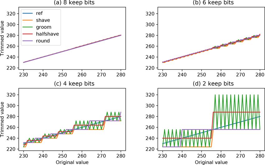
R. Kouznetsov: On precision-preserving compression                                                                               379

and the efficiency of compression improves. Therefore the           one, the result will be equivalent to rounding to infinity; i.e.,
problem of trimming LSBs can be formulated as follows:              it will have an average bias of the value of the most signif-
given an array of floating-point numbers, transform it so that      icant of the tail bits. A rigorous procedure of rounding half
the resulting values have all but N LSBs of their mantissa set      to even (a default rounding mode in IEEE 754) is free from
to a prescribed combination, while the difference from the          biases and should be used.
original array is minimal.                                             The implementations of the abovementioned bit trimming
   Hereafter we will use the term “keep bits” for the N most        and rounding procedures are given in Appendix A.
significant bits of the mantissa, which we use to store the
information from the original values, and “tail bits” for the
remaining bits of a mantissa that we are going to set to a          3   Quantification of errors
prescribed value. The resulting precision is characterized by
the number of bits of the mantissa that we are going to keep.       To characterize the trimming we will use the number of ex-
   The following methods have been considered:                      plicit bits kept in the mantissa of a floating-point number.
                                                                    Therefore “bits = 1” means that the mantissa keeps 1 implicit
  – shave – set all tail bits to 0                                  and 1 explicit bits for the value and the remaining 22 bits
  – set – set all tail bits to 1                                    have been reset to a prescribed combination.
                                                                       When rounding to a fixed quantum (e.g., to integer), the
  – groom – set all tail bits to 1 or to 0 in alternate order for   magnitude of the maximal introduced error is a function of
    every next element of the array                                 the quantum. The error is one quantum for one-sided round-
                                                                    ing (up, down, towards 0, away from 0) and half of the
  – halfshave – set all tail bits to 0 except for the most sig-     quantum for rounding to the nearest value. With precision-
    nificant one of them, which is set to 1                         preserving compression, the quantum depends on the value
  – round – round the mantissa to the nearest value that has        itself. For a value v discretized with M bits of the mantissa
    zero tail bits. Note that this rounding affects keep bits       kept (M − 1 keep bits) the quantum is the value of the least
    and might affect the exponent as well.                          significant bit of keep bits, i.e., at least |21−M v|, and at most
                                                                    |2−M v| depending on how far v is from the maximum power
The first three of these were implemented in NCO some               of 2 that is less than v. Note that the quantization levels for
years ago and are described well by Zender (2016). They             the halfshave method are at midpoints of the intervals be-
can be implemented by applying of bit masks to the origi-           tween the levels for other methods.
nal floating-point numbers. Halfshave and round have been              The shave method implements rounding towards 0. The
recently introduced into NCO. Halfshave is trivial to imple-        set method is almost rounding away from 0. They introduce
ment by applying an integer bit mask to a floating-point num-       an error of at most a full quantum to each value with a mean
ber: the first one applies the shave bit mask and then sets the     absolute error of a half-quantum. The groom method being
MSB of tail bits to 1.                                              alternately shave and set has the same absolute error as those
   Rounding can be implemented with integer operations              but is almost unbiased on average. The round method takes
(Milan Klöwer, personal communication, July 2020). Con-             into account the value of the MSB of tail bits and therefore
sider an unsigned integer that has all bits at 0, except for the    introduces an error of at most a half-quantum with a mean
most significant one of the tail bits. Adding this integer to       absolute error of a quarter of a quantum. The same applies
the original value u, treated as an unsigned integer, would         to the halfshave method, since its levels are midpoints of the
not change the keep bits if u has 0 in the corresponding bit,       range controlled by the tail bits of the original value. Note
and bit shaving of the sum will produce the same result as          that for the mean absolute error estimate we assume that the
bit shaving the original value, i.e., u rounded towards 0. If u     tail bits have an equal chance of being 0 or 1.
has 1 in the corresponding bit, the carry bit will propagate to        The margins of error introduced by the methods for differ-
the fraction or even to the exponent. Bit shaving the result-       ent numbers of mantissa bits are summarized in Table 1. As
ing value is equivalent to rounding u towards infinity. In both     one can see, the round and halfshave methods allow for half
cases the result is half-to-infinity rounding, i.e., rounding to    the error for the same number of keep bits or one less keep
the nearest discretization level, and the value that is exactly     bit to guarantee the same accuracy as shave, set, or groom.
in the middle of a discretization interval would be rounded            The results of applying precision trimming with various
away from 0.                                                        numbers of keep bits are illustrated in Fig. 1, where the 1:1
   Rounding half to infinity introduces a small bias away           line is marked as “ref”. The set method is not shown, to re-
from 0 on average. The magnitude of the bias is half of the         duce the number of lines in the panels. For the shown range
value of the least significant bit of the original number, i.e.,    and keep bits of 8, 4, 6, and 2, the discrete levels are separated
about 10−8 for the single precision. For many applications          by 0.5, 2, 8, and 32, respectively. The levels of halfshave have
such biases can be safely neglected. However, if one applies        a half-discrete offset with respect to the others. For eight keep
such a procedure in a sequence trimming the tail bits one by        bits (Fig. 1a) on the scale of the plots the distortion is almost

https://doi.org/10.5194/gmd-14-377-2021                                                  Geosci. Model Dev., 14, 377–389, 2021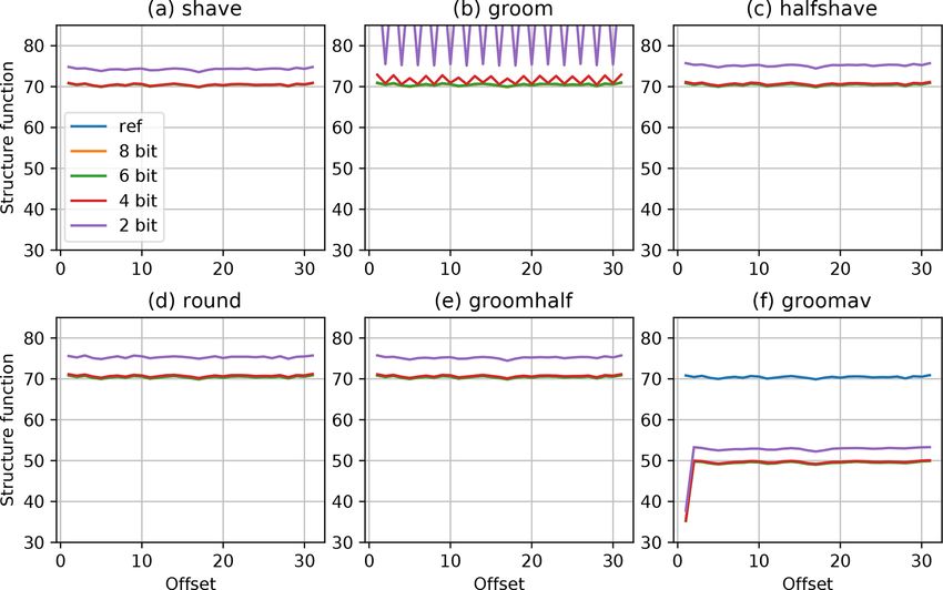
380                                                                         R. Kouznetsov: On precision-preserving compression

Figure 1. Trimmed values as a function of original values when trimmed to different numbers of keep bits. The lines correspond to the
different trimming methods.

Table 1. The discretization level increment for different numbers of the mantissa bits kept and the maximum relative error introduced by
trimming the precision with various methods.

             Mantissa size (bit)   Keep bits   Discretization level increment                 Max relative error
                                               as a fraction of the value
                                                                                     Shave, Set, Groom   Round, Halfshave
                              1           0               0.5   ...              1              100 %                 50 %
                              2           1             0.25    ...            0.5               50 %                 25 %
                              3           2            0.125    ...          0.25                25 %               12.5 %
                              4           3          0.0625     ...         0.125              12.5 %               6.25 %
                              5           4         0.03125     ...        0.0625              6.25 %                3.1 %
                              6           5        0.015625     ...       0.03125                3.1 %               1.6 %
                              7           6      0.0078125      ...     0.015625                 1.6 %               0.8 %
                              8           7     0.00390625      ...    0.0078125                 0.8 %               0.5 %
                              9           8    0.001953125      ...   0.00390625                 0.5 %              0.25 %

invisible, whereas for two keep bits the difference is easily          between two points with both even (or both odd) indices will
seen. Note the increase in the quantum size at 256 due to the          stay unbiased.
increment of the exponent.                                                One can note that the result of applying the halfshave pro-
   It was pointed by Zender (2016) the shave method intro-             cedure with the same number of keep bits to a bit-groomed
duces a bias towards 0, which might be unwanted in some                field is equivalent to applying it to the original field. There-
applications (set introduces the opposite bias). The idea of           fore halfshave can be regarded as a method to halve the error
Bit Grooming (groom) is to combine these two biased trim-              and remove the artifacts of Bit Grooming.
ming procedures to get on average unbiased fields.
   However, it has been overlooked that Bit Grooming intro-
duces an oscillating component that affects multipoint statis-
tics. With Bit Grooming, the quantization of a value in an
array depends not only on the value itself but also on its in-         4   Examples
dex in the array. As a result of this, the absolute difference
between two values with even and odd indices will become               Consider an array of N floating-point numbers ui and its
positively biased on average, while the absolute difference            precision-trimmed version vi . To illustrate the performance
                                                                       of the algorithms we will consider the normalized root-mean-

Geosci. Model Dev., 14, 377–389, 2021                                                     https://doi.org/10.5194/gmd-14-377-2021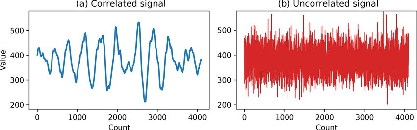
R. Kouznetsov: On precision-preserving compression                                                                                    381

Figure 2. The signals used for illustration (a) correlated and (b) uncorrelated.

Figure 3. The structure functions (Eq. 3) of the correlated signal shown in Fig. 2a, processed with different precision trimmings.

Table 2. NRMSE (normalized root-mean-square error) of the signal          and a distortion to the structure function of the precision-
in Fig. 2a after trimming precision.                                      trimmed fields, which is defined as follows:
                                                                                 v
                 Two keep bits     Four keep bits    Six keep bits               u 1 NX      −r
                                                                                 u
                                                                          X(r) = t              (ui − vi+r )2 ,                    (3)
  Shave                0.09800           0.02479          0.00619                   N − r i=r
  Groom                0.09941           0.02478          0.00620
  Halfshave            0.04968           0.01231          0.00310         where the integer argument r is called offset and can be a
  Round                0.04927           0.01252          0.00311         spatial or temporal coordinate.
  Groomhalf            0.04968           0.01231          0.00310            To illustrate the features of precision trimming, we will use
  Groomav              0.04870           0.01141          0.00280
                                                                          two synthetic arrays: a random process with a “−2”-power
                                                                          spectrum (Fig. 2a) and random Gaussian noise (Fig. 2b). The
                                                                          former is a surrogate of a geophysical signal with high auto-
                                                                          correlation, whereas the latter corresponds to a signal with a
                                                                          large stochastic component. Both signals have identical vari-
square error (NRMSE) introduced by precision trimming,                    ance, which is controlled cut-off at low-frequency compo-
                                                                          nents of the correlated signal and by the variance parameter
                                                                          of the uncorrelated signal. To simplify the analysis we have
                                                                          added a background that is 8 times the signal’s standard devi-
        v
        u    N                                                            ation. Each array is 32 768 values long. The exact code used
        u1 X    (ui − vi )2                                               to generate the signals and all the figures of this paper can be
NRMSE = t                   ,                                    (2)
          N i=1     u2i                                                   found in the Supplement.

https://doi.org/10.5194/gmd-14-377-2021                                                         Geosci. Model Dev., 14, 377–389, 2021
382 R. Kouznetsov: On precision-preserving compression Figure 4. The structure function (Eq. 3) of the signal shown in Fig. 2b, processed with different precision trimmings. The NRMSE of the signal in Fig. 2a after precision trim- July 2020). For a smooth signal, the running average pro- ming with the considered methods is summarized in Ta- duces a structure function that is closer to ref than one for the ble 2. The results fully agree with Table 1: the NRMSE in- mantissa rounding. The steeper structure function for smaller troduced by every method is about half of the maximum er- offsets in Fig 3f is a result of smoothing by the moving aver- ror for a single value. Along with abovementioned methods age. we have added two ways of rectifying bit-groomed values: The situation is different for the uncorrelated random sig- groomhalf, where we apply halfshave to the bit-groomed ar- nal from Fig. 2b, whose structure function is given in Fig. 4. ray, and groomav, where a simple two-point moving average For this signal the reference structure function is flat and the is applied to the data. remaining oscillations are due to the sampling errors. As in As expected, groomhalf results in exactly the same values the previous case, the increase in the number of keep bits as halfshave and therefore has identical NRMSE. The scores makes the structure function closer to the reference one, but for halfshave and round are slightly different due to the lim- the offset also depends strongly on the location of the back- ited sample size and limited number of discrete levels for the ground and the variance with respect to the discretization lev- samples. It is notable that for smooth signals like the one in els. As in the case of the smooth signal, Bit Grooming pro- Fig. 2a, the moving average of bit-groomed values gives a duces oscillating distortions of the structure function, which smaller NRMSE than for all other methods. The reason is in can be removed by applying halfshave. the smoothness of the signal, which has well-correlated ad- The moving average notably reduces the variance of jacent points, while bit-trimming errors are less correlated. the uncorrelated signal, and the structure function becomes For the signal with a “−2”-power spectrum (Fig. 2a) the lower. A dip at the unity offset at Fig 3f is caused by a corre- structure function is linear. The structure functions of the lation between neighboring points introduced by the moving signal processed with trim-precision are given in Fig. 3. All average. Therefore the moving average for poorly correlated panels have the structure function of the original signal (ref signals is more damaging than Bit Grooming. curve) plotted along with curves for the processed signal. Since the structure function is not sensitive to the offsets, the plots for shave, halfshave, and groomhalf (panels a, c, and e) 5 Keeping absolute precision are identical. Panel d differs slightly form them due to statis- tical differences mentioned above. The Bit Grooming algo- Some applications require a given absolute precision, i.e the rithm produces quite large peaks at odd offsets, whereas the acceptable error of data representation is expressed in ab- values at even offsets are equal to the corresponding values solute units rather than as a fraction of a value. For such for shave or halfshave. data, when applying a rounding precision-trimming proce- As a way to compensate for the artifacts of Bit Groom- dure, one can specify the value of the least significant keep ing without introducing additional bias one could apply bit, rather than the fixed number of mantissa bits, and there- moving average (Charles Zender, personal communication fore ensure that the absolute error of the representation will Geosci. Model Dev., 14, 377–389, 2021 https://doi.org/10.5194/gmd-14-377-2021
R. Kouznetsov: On precision-preserving compression                                                                              383

be within a half of that value. The latter method is called the     lected to any value in the range of 0–255 (often only 0–63 are
“decimal significant digit” (DSD) method in NCO (Zender,            implemented). Therefore LP parameters can be optimized for
2016). Since both relative- and absolute-precision-trimming         each field to provide the required absolute precision. Writing
methods reset least significant bits of floating-point values,      of large GRIB datasets can be done field by field in a single
the statistical properties of the distortions introduced by these   pass. The approach has been widely used and works well for
methods are similar.                                                meteorological data. Recent GRIB2 standards enable a loss-
   If the required accuracy of a variable is given in terms         less data compression of packed data with the CCSDS/AEC
of both relative and absolute precision, precision trimming         (Consultative Committee for Space Data Systems/Adaptive
with a limit for both the least significant keep-bit number         Entropy Coding) algorithm, which provides further reduction
and the least significant keep-bit value can be used. This can      in the packed data size for a typical output of a numerical-
be achieved by sequential application of the two trimming           weather-prediction model by about a half (50 %–60 % of re-
procedures.                                                         duction in our experience). This compression alleviates the
                                                                    use of redundant bitsPerValue when the absolute preci-
                                                                    sion is specified (option 2 above), and therefore the GRIB2
6    Precision of linear packing                                    implementation of LP is good for data of a limited dynamic
                                                                    range and a requirement for absolute precision.
Linear packing (LP) is a procedure of applying a linear trans-
                                                                       LP for the classic NetCDF format has additional impli-
formation that maps the range of the original values onto the
                                                                    cations. The format provides a choice of 8, 16, or 32 bits
representable range of an integer data type and rounds and
                                                                    per value for integers, and the integers are signed. According
stores the resulting integers. The parameters of the transfor-
                                                                    to the CF conventions (http://cfconventions.org; last access:
mation – the offset and scale factor – have to be stored for
                                                                    19 January 2021), LP applies the same linear transformation
subsequent recovery of the data. The method itself leads to a
                                                                    parameters for the whole variable in a file which may contain
reduction in the dataset size if the integer size is shorter than
                                                                    many levels and/or time steps. Many implementations (e.g.,
the original floating-point size. Applying a lossless compres-
                                                                    the ncpdq tool from NCO) use option 1 from above, there-
sion to the resulting integer array usually leads to further re-
                                                                    fore requiring two passes through the dataset, which might
duction in size.
                                                                    require a consideration of memory constraints. This way usu-
   When applying LP to a dataset one has to select the pa-
                                                                    ally does not lead to noticeable artifacts for common meteo-
rameters of the transformation and a size of the integer data
                                                                    rological variables. However, if the original field has a large
type (bitsPerValue parameter). This can be done in two
                                                                    dynamic range or has a substantially skewed distribution, the
ways:
                                                                    errors in LP can be huge.
    1. One can specify bitsPerValue and map the range of               Consider a gridded field of in-air concentration of a pol-
       an array onto the representable range. In this case a full   lutant continuously emitted from a point source in the atmo-
       array has to be analyzed prior to the packing, and the ab-   sphere. The maximum value of such a field would depend
       solute precision of the representation will be controlled    on a grid resolution, and the number of bits needed to pack
       by the difference between the maximum and minimum            such a field with a given relative or absolute accuracy has to
       values of the array. This approach is acceptable when        be decided on a case-by-case basis. Moreover, if one needed
       the encoded parameter is known to have a certain range       to integrate such a field to get the total emitted mass of the
       of values; then the resulting errors can be reliably con-    pollutant, the integral of the unpacked field could be very dif-
       strained.                                                    ferent from the integral of the original field. If the zero value
                                                                    of the original field can be exactly represented as a packed
    2. One can explicitly specify the required absolute preci-
                                                                    value, a substantial fraction of mass can be hidden in near-
       sion of the representation by pre-defining the scale fac-
                                                                    zero values. If the zero value of the original field is mapped
       tor. Then a number of bitsPerValue has to be taken
                                                                    to a (“small”) non-zero value, the total mass, obtained from
       with a sufficient margin to ensure that all values can be
                                                                    integration of the unpacked field, would depend on the do-
       mapped onto the representable range.
                                                                    main size.
In both cases LP controls the absolute error of the repre-             Rounding errors in linear packing can lead to unphysical
sentation, which makes LP suboptimal for the data that re-          values. Consider a single-precision field (of, e.g., humidity)
quire a constraint for a relative error. If a dataset has a         that has values between 0 and 0.99999535. If one packs it to
large dynamic range (many orders of magnitude), the num-            an 8-bit signed integer (byte) with the standard procedure of
ber of bitsPerValue might become larger than the bit                NCO (as in version 4.9.4) and unpacks it back with the same
size of the original floating-point values, if they are at all      NCO, one obtains −2.980232 × 10⁻⁸ as the minimum value
representable with a specific output format (e.g., 32 bits for      instead of 0. The negative value results from rounding errors
NetCDF).                                                            and a finite precision of the packing parameters. An unphys-
   GRIB format allows for applying LP to individual gridded         ical value used in a model might lead to arbitrary results.
2D fields, and the bitsPerValue parameter can be se-                If the variable has a specified valid_range attribute, CF

https://doi.org/10.5194/gmd-14-377-2021                                                  Geosci. Model Dev., 14, 377–389, 2021
384 R. Kouznetsov: On precision-preserving compression
conventions prescribe treating the corresponding values as likely to differ between neighboring points. For the example
missing. arrays the monotonicity breaks between 0 and 1 keep bits
Therefore we conclude that LP produces acceptable results since for 0 keep bits, the rounding procedure alters the ex-
when the required margin for absolute errors is within a few ponent, which stays constant otherwise. Some of the curves
orders of the field’s maximum value and if the valid range have a noticeable dip in the compressed size at 7 and 15 keep
of a variable covers the actual range with that margin. In a bits, corresponding to byte boundaries. The dip is mostly pro-
general case, the application of LP might lead to errors of nounced for zlib compression.
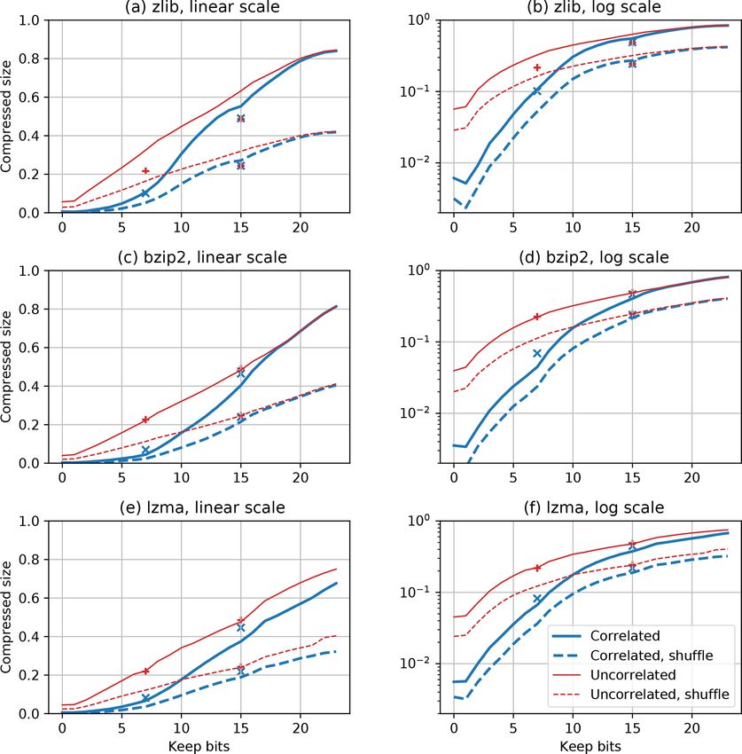
arbitrary magnitude or can make valid data invalid. Shuffling substantially improves the compression effi-
A useful application of the packing parameters is scaling ciency and leads to a twice smaller resulting size for our
or unit conversion for the data that already have trimmed pre- datasets for all compression methods, including linear pack-
cision. If one multiplies precision-trimmed data with a factor ing to 16 bits. The reason is that general-purpose compres-
that differs form a power of 2, the scaling also affects the tail sion algorithms operate on the data as a sequence of bytes,
bits and the compression efficiency reduces. However, if one and grouping corresponding bytes facilitates the recognition
scales the data by altering the scale_factor attribute of a of repeating patterns in the data flow.
NetCDF file, the stored array stays intact and well compress- At high precisions the compression algorithms do not take
ible, and CF-aware readers will apply the scaling on reading. advantage of the correlated signal and both signals have the
same compression ratio, except for lzma, which is the most
expensive of all three. The difference between the signals is
7 Compressing precision-trimmed data also small for 16-bit linear packing. At lower precisions the
correlated array compresses notably better than the uncorre-
To give an example of the storage-space savings due to com- lated one.
pression we compressed the test arrays shown in Fig. 2 pro- Compression of linearly packed data does only marginally
cessed with mantissa rounding and plotted the compressed- better for the correlated array at 16 bits, while it makes a no-
data size as a function of the number of keep bits. The table difference between the arrays at 8-bit resolution. Lin-
size is normalized with the storage size of the original array ear packing of the uncorrelated array at 16 bits leads to some
(32 768×4 bytes). We used three compression methods avail- 15 % better zlib compression than corresponding precision
able from the standard Python library: zlib (the same as used trimming; for the correlated array the difference is much
with NetCDF4 compression) with level 6, bzip2, and lzma. smaller. In all other cases the precision-trimming results in
The latter two are more expensive computationally but pro- the same or better compressions than the corresponding shuf-
vide a higher compression ratio and can be applied to com- fled packed array.
press the raw binary data files or used in future data formats.
To emulate the compression used with NetCDF4 we have
applied shuffling to the bit-trimmed arrays. Shuffling is a pro- 8 Practical examples
cedure of re-arrangement of the data bytes in a floating-point
array, so they get ordered sequentially: all first bytes of each Lossy compression is a compromise between the accuracy
number, then all second bytes, etc. The procedure is known and the compression efficiency. Optimal parameters of com-
to improve the compression ratio in most cases. Shuffling has pression depend on the nature of the data and on the in-
been available in the NetCDF4 library and is applied in NCO tended application. In this section we give examples on suit-
in writing compressed variables. able compression parameters for several practical applica-
Figure 5 shows the compression ratio for the precision- tions. For illustrations we use some atmospheric variables
trimmed test signals with (dashed lines) and without (solid that the author dealt with.
lines) shuffling processed with three compression methods. Consider gridded fields of the 2 m temperature and the
We used mantissa rounding with the number of keep bits surface-air pressure in the Earth atmosphere. The fields have
from 0 to 23, i.e., the full range of possible trimmings for a limited dynamic range: the values of pressure fall within
single-precision floats. To better visualize the full range of 330 hPa (at the Everest summit) and 1065 hPa (at Dead Sea
compression ratios we plot them in both linear and logarith- level), and for the temperature the range is 200 to 360 K.
mic scales. For a reference the compressed-size of the same For such fields the spacing of quantization levels for preci-
arrays packed with linear packing to 8- and 16-bit signed in- sion trimming falls within a factor of 2–4, and to achieve the
tegers is shown. The packed data are attributed to the number same norm of absolute (or relative) precision one would need
of keep bits corresponding to the same maximum absolute approximately the same number of mantissa bits for preci-
error. sion trimming or bits per value for linear packing. The fields
For all algorithms the reduction in keep bits leads to the are usually smooth, so the most significant bits do not differ
reduction in compressed size. The reduction is nearly linear among neighboring cells, and a subsequent lossless compres-
for the uncorrelated signal and faster than linear for the cor- sion yields a substantial gain in size even with a large number
related signal, since more significant bits of the latter are less of bits kept.
Geosci. Model Dev., 14, 377–389, 2021 https://doi.org/10.5194/gmd-14-377-2021R. Kouznetsov: On precision-preserving compression 385
Figure 5. The normalized compressed size (compression ratios) of the arrays shown in Fig. 2, as a function of the number of keep bits
for mantissa rounding with and without shuffling. Compression ratios for same arrays packed with linear packing are shown with points of
respective color. The ratios are shown both in linear and logarithmic scale for three compression methods. Twenty-three keep bits correspond
to the original precision.
Suppose the intended use of the dataset is the calculation or wind energy one would need a precision exceeding the
of the components of a geostrophic wind ug , vg , defined as precision of reference wind measurements. Best atmospheric
(Holton and Hakim, 2013) cup anemometers have about 1 % relative accuracy and about
1 cm s−1 absolute accuracy. If we neglect representativeness
1 ∂p 1 ∂p error, which is usually larger than an instrument error but less
−f vg ' − ; −f ug ' − , (4)
ρ ∂x ρ ∂y trivial to evaluate, one would need six to seven mantissa bits
for the model wind components. If one is going to reconstruct
where f ' 10−4 s is a Coriolis parameter and ρ is the air
the vertical wind component from the horizontal ones using
density. If the target accuracy for the geostrophic wind is
the continuity equation, e.g., for offline dispersion modeling,
0.1 m s−1 or 1 % and the grid spacing is 10 km, one would
the required precision of horizontal components is absolute
need the pressure accurate within 0.01 hPa and temperature
and depends on the grid resolution, similarly to the afore-
within 2 K. Therefore 17 mantissa bits will be needed for the
mentioned case of geostrophic wind.
pressure, while only 6 bits are needed for the temperature.
One could note that relative-precision trimming leaves
However, if both fields are needed to convert between the
excess precision for small absolute values of wind and is
volume mixing ratio and the mass concentration of an atmo-
therefore suboptimal for data compression. The absolute-
spheric trace gas, whose measurements are accurate within,
precision trimming should be more appropriate for wind
e.g., 1 %, six to seven bits per value will be sufficient for both
components. Since the range of wind components in the at-
variables.
mosphere is limited, linear packing has been successfully
Another example is wind components from a meteorolog-
used for wind components without major issues. Archives
ical model. For practical applications, like civil engineering
https://doi.org/10.5194/gmd-14-377-2021 Geosci. Model Dev., 14, 377–389, 2021386 R. Kouznetsov: On precision-preserving compression
of numerical weather prediction (NWP) forecasts typically given relative precision, we considered absolute-precision
use linear packing with 16–18 bits per value for wind com- trimming that specifies a value for the least significant man-
ponents. tissa bit. The latter method is recommended when required
In the aforementioned case of a concentration field origi- absolute precision is specified. Depending on the nature of a
nating from a point source, where LP is inapplicable, preci- variable in the dataset and intended application either or both
sion trimming works well. Precision trimming does not affect of the trimmings can be applied to remove non-significant
the representable dynamic range of the field, and the relative information and achieve the best compression performance.
precision of the integral of the field over some areas is at least Precision trimming and subsequent lossless compression
the same as one of the precision-trimmed data. has substantial advantages over the widely used linear pack-
Often, in problems of atmospheric dispersion, both the ing method: it allows us to explicitly specify the required pre-
emission sources and observations have quite large uncer- cision in terms of both absolute and relative precision, guar-
tainty; therefore there is no reason to keep a large number antees to keep the sign and a valid range of an initial value,
of significant figures in simulation results. If one creates a and allows for the use of the full range of floating-point val-
lookup database for scenarios of an emergency release of ues. Our examples illustrate that linear packing can lead to
hazardous materials at various meteorological conditions, the unconstrained errors and does not provide substantial sav-
database size is one of the major concerns, while the uncer- ings in the storage space over precision trimming; therefore
tainty of the released amount is huge. For such applications linear packing should be considered deprecated. The excep-
even 1–2 keep bits for the concentration fields can be suffi- tion is GRIB2, where linear packing is applied to individual
cient. 2D fields of known dynamic range, uses unsigned integers of
For model–measurement comparisons of such simulations arbitrary length, and involves specialized compression algo-
one might be interested only in concentrations exceeding rithms.
some threshold, e.g., some fraction of the detection limit of The precision-trimming methods described in the paper
the best imaginable observation. Then in addition to trim- were implemented in Python, and corresponding subroutines
ming relative precision, one could trim the absolute preci- are given in the Appendix, where we also put subroutines
sion of the field and therefore zero-out a substantial part of for relative- and absolute-precision trimming with mantissa
the model domain, further reducing the dataset storage size. rounding, implemented with Fortran 95 intrinsics. The sub-
routines should be directly usable in various geoscientific
models.
9 Conclusions
A simple method for trimming precision by rounding a man-
tissa of floating-point numbers has been implemented and
tested. It has been incorporated into the NCO mainstream
and has been used by default since v 4.9.4. The method has
half the quantization error of the Bit Grooming method (Zen-
der, 2016), which was used by default in earlier versions of
NCO. Bit Grooming, besides having suboptimal precision,
leads to substantial distortion of multipoint statistics in sci-
entific datasets. The “halfshave” procedure can be used to
partially recover the precision and remove excess distortions
from two-point statistics of bit-groomed datasets.
Precision trimming should be applied to data arrays before
feeding them to NetCDF or any another data-output library.
The trimming can be applied to any data format, e.g., raw bi-
nary, that stores arrays of floating-point numbers to facilitate
subsequent compression. NCO provides a limited leverage to
control the number of mantissa bits in terms of specifying “a
number of significant digits” (SD) for a variable. These dig-
its can be loosely translated into the number of mantissa bits:
1 SD is 6 bits, 2 SD is 9 bits, 3 SD is 12 bits, etc. The exact
translation varies slightly among the NCO versions; there-
fore low-level data processing should be used if one needs to
control the exact number of mantissa bits to keep.
Along with a relative-precision trimming that keeps a
given number of mantissa bits and therefore guarantees a
Geosci. Model Dev., 14, 377–389, 2021 https://doi.org/10.5194/gmd-14-377-2021R. Kouznetsov: On precision-preserving compression 387 Appendix A: Implementation of precision trimming mask = (0xFFFFFFFF>>maskbits)
388                                               R. Kouznetsov: On precision-preserving compression

subroutine trim_abs_precision(a, max_abs_err)

      real (kind=4), dimension(:), &
                     & intent(inout) :: a
      real, intent(in) :: max_abs_err
      real :: log2maxerr, quantum, a_maxtrimmed

      log2maxerr = log(max_abs_err)/log(2.)
      quantum = 2.**(floor(log2maxerr)+1.)

      !! Avoid integer overflow
      a_maxtrimmed = quantum * 2**24
      where (abs(a) < a_maxtrimmed) &
         & a = quantum * nint(a / quantum)

end subroutine trim_abs_precision

Geosci. Model Dev., 14, 377–389, 2021                        https://doi.org/10.5194/gmd-14-377-2021
R. Kouznetsov: On precision-preserving compression 389
Code availability. The implementation of mantissa rounding in C References
has been introduced into the NCO master branch. The source code
of NCO is available from http://nco.sourceforge.net (last access: ANSI/IEEE: IEEE Standard for Binary Floating-Point
7 December 2020) under BSD license. The Python3 code used to Arithmetic, ANSI/IEEE Std 754-1985, pp. 1–20,
generate the figures and the example statistics is available from the https://doi.org/10.1109/IEEESTD.1985.82928, 1985.
Supplement and can be used under the BSD license. Holton, J. and Hakim, G.: An Introduction to Dynamic Meteo-
rology, Academic Press, Elsevier Science, Amsterdam, Boston,
Heidelberg, London, New York, Oxford, Paris, San Diego, San
Supplement. The supplement related to this article is available on- Francisco, Singapore, Sydney, Tokyo, 2013.
line at: https://doi.org/10.5194/gmd-14-377-2021-supplement. Stackpole, J. D.: GRIB (Edition 1) The WMO Format for the
Storage of Weather Product Information and the Exchange of
Weather Product Messages in Gridded Binary Form, Office note
388, U.S. Department of Commerce, National Oceanic and At-
Competing interests. The author declares that there is no conflict of
mospheric Administration, National Weather Service, National
interest.
Meteorological Center, MD, USA, 1994.
Zender, C. S.: Bit Grooming: statistically accurate precision-
preserving quantization with compression, evaluated in the
Acknowledgements. I would like to thank Mikhail Sofiev netCDF Operators (NCO, v4.4.8+), Geosci. Model Dev., 9,
and Viktoria Sofieva from the Finnish Meteorological Insti- 3199–3211, https://doi.org/10.5194/gmd-9-3199-2016, 2016.
tute and Dmitrii Kouznetsov from the University of Electro-
Communications, Tokyo, for fruitful discussions and Charles Zen-
der from the University of California for the NetCDF Operator
software (NCO) and for being open and swift about verifying and
accepting the patches for it. Also, I am grateful to Milan Klöwer
from Oxford University, Mario Acosta from the Barcelona Su-
percomputer Center, Seth McGinnis from the National Center
for Atmospheric Research, and Ananda Kumar Das from the
Indian Meteorological Department for their careful reading of the
discussion paper and their critical and valuable comments. The
initial implementation of mantissa rounding for the SILAM model
was done within the “Global health risks related to atmospheric
composition and weather, GLORIA” project from the Academy
of Finland (grant 310373). Adaptation of the mantissa rounding
for absolute precision was made for the Russian Foundation for
Basic Research “Experimental studies of internal gravity waves
in the mid-altitude atmospheric boundary layer” (project no. 19-
05-01008). The detailed analysis of the precision trimming was
performed within the service contract CAMS_61 “Development
of regional air quality modelling and data assimilation aspects”
of the Copernicus Atmosphere Monitoring Service (contract
notice 2019/S 118-289635).
Review statement. This paper was edited by Paul Ullrich and re-
viewed by Ananda Kumar Das, Mario Acosta, and Seth McGinnis.
https://doi.org/10.5194/gmd-14-377-2021 Geosci. Model Dev., 14, 377–389, 2021You can also read