Reducing the Sampling Complexity of Topic Models
←
→
Page content transcription
If your browser does not render page correctly, please read the page content below
Reducing the Sampling Complexity of Topic Models

                                                         Aaron Q. Li                                     Amr Ahmed
                                           CMU Language Technologies                            Google Strategic Technologies
                                                 Pittsburgh, PA                                      Mountain View, CA
                                                  aaronli@cmu.edu                                    amra@google.com
                                                     Sujith Ravi                                     Alexander J. Smola
                                          Google Strategic Technologies                           CMU MLD and Google ST
                                               Mountain View, CA                                      Pittsburgh PA
                                                  sravi@google.com                                     alex@smola.org

ABSTRACT                                                                                         with the data. A substantial improvement in this context
Inference in topic models typically involves a sampling step                                     was provided by [22] who exploited sparsity to decompose
to associate latent variables with observations. Unfortu-                                        the collapsed sampler [9] for Latent Dirichlet Allocation. As
nately the generative model loses sparsity as the amount                                         a result the sampling cost can be reduced from O(k), the
of data increases, requiring O(k) operations per word for k                                      total number of topics to O(kd + kw ), i.e. the number kw of
topics. In this paper we propose an algorithm which scales                                       topics occurring for a particular word w and kd for a partic-
linearly with the number of actually instantiated topics kd in                                   ular document d. This insight led to an order of magnitude
the document. For large document collections and in struc-                                       improvement for sampling topic models, thus making their
tured hierarchical models kd  k. This yields an order of                                        implementation feasible at a large scale. In fact, the strat-
magnitude speedup. Our method applies to a wide variety                                          egy is sufficiently robust that it can be extended to settings
of statistical models such as PDP [16, 4] and HDP [19].                                          where the topic smoother depends on the words [15].
   At its core is the idea that dense, slowly changing distri-                                      For small datasets the assumption kd +kw  k is well sat-
butions can be approximated efficiently by the combination                                       isfied. Unfortunately, as the number of documents grows, so
of a Metropolis-Hastings step, use of sparsity, and amortized                                    does the number of topics in which a particular word occurs.
constant time sampling via Walker’s alias method.                                                In particular kw → k, since the probability of observing any
                                                                                                 particular topic for a given word is rarely nonzero: Assume
                                                                                                 that the probability of occurrence for a given topic for a
Keywords                                                                                         word is bounded from below by δ. Then the probability of
Sampling; Scalability; Topic Models; Alias Method                                                the topic occurring at least once in a collection of n docu-
                                                                                                 ments is given by
1.      INTRODUCTION                                                                                       1 − (1 − δ)n ≥ 1 − e−nδ → 1 for n → ∞.
   Topic models are some of the most versatile tools for mod-
eling statistical dependencies. Given a set of observations                                      From this it follows that kw = O(k) for n = O(δ −1 log k).
xi ∈ X , such as documents, logs of user activity, or com-                                       In other words, for large numbers documents the efficiencies
munications patterns, we want to infer the hidden causes                                         discussed in [22] vanish. This is troubling, since in many in-
motivating this behavior. A key property in topic models                                         dustrial settings n can be in the order of billions to trillions.
is that they model p(x) via a discrete hidden factor, z via                                      Consequently, with increasing amounts of data, the time to
p(x|z) and p(z). For instance, z may be the cluster of a docu-                                   process individual documents increases due to loss of spar-
ment. In this case it leads to Gaussian and Dirichlet mixture                                    sity, thus leading to a superlinear increase in runtime.
models [14]. When z is a vector of topics associated with in-                                       On the other hand, the topic-sparsity for a given document
dividual words, this leads to Latent Dirichlet Allocation [3].                                   essentially remains unchanged, regardless of the total num-
Likewise, whenever z indicates a term in a hierarchy, it leads                                   ber of related documents that are available. This is due to
to structured and mixed-content annotations [19, 2, 4, 12].                                      the fact that the number of tokens per document is typically
                                                                                                 less than O(k). For instance, microblogs contain only dozens
1.1       Sparsity in Topic Models                                                               of words, yet admit to thousands of topics.1 This situation
  One of the key obstacles in performing scalable inference is                                   is exacerbated when it comes to hierarchical and structured
to draw p(z|x) from the discrete state distribution associated                                   topic models, since there the number of (sub)topics can grow
Permission to make digital or hard copies of all or part of this work for personal or            considerably more rapidly. Hence the use of sparsity is cru-
classroom use is granted without fee provided that copies are not made or distributed            cial in designing efficient samplers.
for profit or commercial advantage and that copies bear this notice and the full citation
on the first page. Copyrights for components of this work owned by others than the               1.2    Metropolis-Hastings-Walker Sampling
author(s) must be honored. Abstracting with credit is permitted. To copy otherwise, or
republish, to post on servers or to redistribute to lists, requires prior specific permission      The present paper proposes a new decomposition of the
and/or a fee. Request permissions from permissions@acm.org.                                      collapsed conditional probability, in conjunction with a
KDD’14, August 24–27, 2014, New York, NY, USA.                                                   1
Copyright is held by the owner/author(s). Publication rights licensed to ACM.                      Obviously, this approach would not work to infer topics for
ACM 978-1-4503-2956-9/14/08 ...$15.00.                                                           Dostojevski’s War and Peace. That said, a plain topic model
http://dx.doi.org/10.1145/2623330.2623756.                                                       is an unlikely candidate to represent very long documents.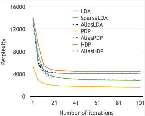
Metropolis-Hastings [7] scheme and the use of the alias             Draw a word from the multinomial ψzdi via
method, introduced by Walker [20, 13], to amortize dense
updates for random variables. This method is highly ver-                                  wdi ∼ Discrete(ψzdi ).                (4)
satile. It defers corrections to the model and avoids renor-
malization. This allows us to apply it to both flat and hier-       The beauty of the Dirichlet-multinomial design is that the
archical models. Experimental evaluation demonstrates the           distributions are conjugate. This means that the multino-
efficacy of our approach, yielding orders of magnitude accel-       mial distributions θd and ψk can be integrated out, thus
eration and a simplified algorithm.                                 allowing one to express p(w, z|α, β, nd ) in closed-form [9].
   While we introduce our algorithm in the context of topic         This yields a Gibbs sampler to draw p(zdi |rest) efficiently.
models, it is entirely general and applies to a much richer         The conditional probability is given by
class of models. At its heart lies the insight that in many
inference problems the model parameters only change rela-                                        (n−di        −di
                                                                                                   td + αt )(ntw + βw )
tively slowly during sampling. For instance, the location of                   p(zdi |rest) ∝                           .       (5)
                                                                                                       n−di
                                                                                                        t    + β̄
cluster centers, the definition of topics, or the shape of au-
toregressive functions, only change relatively slowly. Hence,       Here the count variables ntd , ntw and nt denote the num-
if we could draw from a distribution over k outcomes k times,       ber of occurrences of a particular (topic,document) and
Walker’s alias method would allow us to generate samples in         (topic,word) pair, or of a particular topic respectively. More-
amortized constant time. At the same time, the Metropolis           over, the superscript ·−di denotes said count when ignoring
Hastings algorithm allows us to use approximations of the           the pair (zdi , wdi ). For instance, n−di
                                                                                                          tw is obtained when ignor-
correct probability distribution, provided that we compute          ing the
                                                                         P (topic,word) combination at position (d, i). Finally,
ratios between successive states correctly. Our approach is         β̄ := w βw denotes the joint normalization.
to draw from the stale distribution in constant time and to            At first glance, sampling from (5) appears to cost O(k)
accept the transition based on the ratio between successive         time since we have k nonzero terms in a sum that needs to be
states. This step takes constant time. Moreover, the pro-           normalized. [22] devised an ingenious strategy for exploiting
posal is independent of the current state. Once k samples           sparsity by decomposing terms into
have been drawn, we simply update the alias table. In honor
                                                                                                                           −di
of the constitutent algorithms we refer to our technique as                                αt        −di    βw        −di ntd + αt
                                                                    p(zdi |rest) ∝ βw             + ntd            + ntw
the Metropolis Hastings Walker (MHW) sampler.                                           n−di + β̄        n−di + β̄        n−di + β̄
                                                                                         t                t                 t

                                                                    As can be seen, for small collections of documents     only the
2.    TOPIC MODELS                                                  first term is dense, and Pmore specifically, t αt /(n−di
                                                                                                                  P
                                                                                                                           t   + β̄)
   We begin with a brief introduction to topic models and the       can be computed from t αt /(nt + β̄) in O(1) time. That
associated inference problems. This includes a short motiva-        is, whenever both ntd and ntw are sparse, sampling from
tion of sampling schemes in the context collapsed samplers          p(zdi |rest) can be accomplished efficiently. The use of packed
[9, 18] and of stochastic variational models [21]. It is followed   index variables and a clever reordering of (topic,count) pairs
by a description of extensions to hierarchical models.              further improve efficient sampling to O(kw + kd ).
                                                                       Stochastic variational inference [11] requires an analogous
2.1       Latent Dirichlet Allocation                               sampling step. The main difference being that rather than
   In LDA [3] one assumes that documents are mixture dis-           using ntw   +βw
                                                                             nt +β̄
                                                                                    to capture p(w|t) one uses a natural parameter
tributions of language models associated with individual            ηtw associated with the conjugate variational distribution.
topics. That is, the documents are generated following the          Unfortunately this renders the model dense, unless rather
graphical model below:                                              careful precautions are undertaken [11] to separate residual
                                                                    dense and sparse components.
                                                                       Instead, we devise a sampler to draw from p(zdi |rest) in
                                                                    amortized O(kd ) time. We accomplish this by using
      α       θd      zdi           wdi        ψk        β
                                                                                                 n−di
                                                                                                  tw + βw   αt (n−di
                                                                                                                  tw + βw )
                            for all i        for all k                     p(zdi |rest) ∝ n−di
                                                                                           td      −di
                                                                                                          +                     (6)
                     for all d                                                                   nt + β̄       n−di
                                                                                                                 t   + β̄
For each document d draw a topic distribution θd from a             Here the first term is sparse in kd and we can draw from it
Dirichlet distribution with concentration parameter α               in O(kd ) time. The second term is dense, regardless of the
                                                                    number of documents (this holds true for stochastic varia-
                      θd ∼ Dir(α).                           (1)    tional samplers, too). However, the ’language model’ p(w|t)
                                                                    does not change too drastically whenever we resample a sin-
For each topic t draw a word distribution from a Dirichlet          gle word. The number of words is huge, hence the amount of
distribution with concentration parameter β                         change per word is concomitantly small. This insight forms
                                                                    the basis for applying Metropolis-Hastings-Walker sampling.
                      ψt ∼ Dir(β).                           (2)
                                                                    2.2    Poisson Dirichlet Process
For each word i ∈ {1 . . . nd } in document d draw a topic             To illustrate the fact that the MHW sampler also works
from the multinomial θd via                                         with models containing a dense generative part, we describe
                                                                    its application to the Poisson Dirichlet Process [4, 16]. The
                     zdi ∼ Discrete(θd ).                    (3)    model is given by the following variant of the LDA model:
if no additional ’table’ is opened by word wdi . Otherwise
α θd zdi wdi ψt ψ0 β p(zdi = t, rdi = 1|rest) (8)
m +1
for all i bt + at st stw + 1 γ + stw Sstwtw+1,at
for all k ∝(αt + ndt )
for all d
bt + mt mtw + 1 γ̄ + st Ssmtwtw,at
In a conventional topic model the language model is sim-
N
ply given by a multinomial draw from a Dirichlet distribu- Here SM,a is the generalized Stirling number. It is given by
tion. This fails to exploit distribution information between N +1 N N N
topics, such as the fact that all topics have the same common SM,a = SM −1,a + (N − M a)SM,a and SM,a = 0
underlying language. A means for addressing this problem N
for M > N , and S0,a = δN,0 .P
A detailed analysisPis given in
is to add
Q a level of hierarchy to model the Q distribution over [4]. Moreover we have mt = w mtw , and st = t stw .
ψt via t p(ψt |ψ0 )p(ψ0 |β) rather than t p(ψt |β). Such a
Similar to the conditional probability expression in LDA,
model is depicted above.
these two expressions can be written as a combination of
The ingredients for a refined language model are a Pitman-
a sparse term and a dense term, simply by splitting the
Yor Topic Model (PYTM) [17] that is more appropriate to
factor (αt + ndt ) into its sparse component ndt and its dense
deal with natural languages. This is then combined with
counterpart αt . Hence we can apply the same strategy as
the Poisson Dirichlet Process (PDP) [16, 4] to capture the
before when sampling topics from LDA, albeit now using a
fact that the number of occurences of a word in a natu-
twice as large space of state variables.
ral language corpus follows power-law. Within a corpus, the
frequency of a word is approximately inversely proportional 2.3 Hierarchical Dirichlet Process
to its ranking in number of occurences. Each draw from a
Poisson Dirichlet Process PDP(b, a, ψ0 ) is a probability dis- To illustrate the efficacy and generality of our approach we
tribution. The base distribution ψ0 defines the common un- discuss a third case where the document model itself is more
derlying distribution shared across the generated distribu- sophisticated than a simple collapsed Dirichlet-multinomial.
tions. Under the settings of Pitman-Yor Topic Model, each We demonstrate that there, too, inference can be performed
topic defines a distribution over words, and the base dis- efficiently. Consider the two-level topic model based on the
tribution defines the common underlying common language Hierarchical Dirichlet Process [19] (HDP-LDA). In it, the
model shared by the topics. The concentration parameter topic distribution for each document θd is drawn from a
b controls how likely a word is to occur again while being Dirichlet process DP(b1 , θ0 ). In turn, θ0 is drawn from a
sampled from the generated distribution. The discount pa- Dirichlet process DP(b0 , H(·)) governing the distribution
rameter a prevents a word to be sampled too often by im- over topics. In other words, we add an extra level of hierar-
posing a penalty on its probability based on its frequency. chy on the document side (compared to the extra hierarchy
The combined model described explicityly in [5]: on the language model used in the PDP).
θd ∼ Dir(α) ψ0 ∼ Dir(β)
zdi ∼ Discrete(θd ) ψt ∼ PDP(b, a, ψ0 )
H θ0 θd zdi wdi ψk β
wdi ∼ Discrete (ψzdi )
for all i for all k
As can be seen, the document-specific part is identical to for all d
LDA whereas the language model is rather more sophisti- More formally, the joint distribution is as follows:
cated. Likewise, the collapsed inference scheme is analogous
to a Chinese Restaurant Process [6, 5]. The technical diffi- θ0 ∼ DP(b0 , H(·)) ψt ∼ Dir(β)
culty arises from the fact that we are dealing with distribu- θd ∼ DP(b1 , θ0 )
tions over countable domains. Hence, we need to keep track
zdi ∼ Discrete(θd )
of multiplicities, i.e. whether any given token is drawn from
βi or β0 . This will require the introduction of additional wdi ∼ Discrete (ψzdi )
count variables in the collapsed inference algorithm.
By construction, DP(b0 , H(·)) is a Dirichlet Process, equiva-
Each topic is equivalent to a restaurant. Each token in the
lent to a Poisson Dirichlet Process PDP(b0 , a, H(·)) with the
document is equivalent to a customer. Each type of word
discount parameter a set to 0. The base distribution H(.) is
corresponds each type of dish served by the restaurant. The
often assumed to be a uniform distribution in most cases.
same results in [6] can be used to derive the conditional
At first, a base θ0 is drawn from DP(b0 , H(·)). This gov-
probability by introducing axillary variables:
erns how many topics there are in general, and what their
• stw denotes the number of tables serving dish w in overall prevalence is. The latter is then used in the next level
restaurant t. Here t is the equivalent of a topic. of the hierarchy to draw a document-specific distribution θd
• rdi indicates whether wdi opens a new table in the that serves the same role as in LDA. The main difference is
restaurant or not (to deal with multiplicities). that unlike in LDA, we use θ0 to infer which topics are more
• mtw denotes the number of times dish w has been popular than others.
served in restaurant t (analogously to nwk in LDA). It is also possible to extend the model to more than two
levels of hierarchy, such as the infinite mixture model [19].
The conditional probability is given by: Similar to Poisson Dirichlet Process, an equivalent Chinese
Restaurant Franchise analogy [6, 19] exists for Hierarchi-
αt + ndt mtw + 1 − stw Ssmtwtw,a+1
t cal Dirichlet Process with multiple levels. In this analogy,
p(zdi = t, rdi = 0|rest) ∝ (7)
bt + mt mtw + 1 Ssmtwtw,at each Dirichlet Process is mapped to a single Chinese Restau-rant Process, and the hierarchical structure is constructed This amounts to the following (unnormalized) conditional
to identify the parent and children of each restaurant. probabilities. See [6] for further details.
The general (collapsed) structure is as follows: let Nj be
the total number of customers in restaurant j and njt be p (zdi = t, udi = u|rest) (9)
the number of customers in restaurant j served with dish b0 b1
if st = 0 and udi = 1
b0 +s
t. When a new customer (a token) enters restaurant j with
b1 s 2
the corresponding Dirichlet Process DP (bj , Hj (·)), there are βw + mtw (s +1)(s+b
t
if st 6= 0 and std = 0
two types of seating arrangement for the customer: ∝ t 0)
β̄ + mt n +1
njt
S dt+1,0 s +1
sdt
• With probability bj +N j
the customer is served with
ndt
dt
ndk +1
if st 6= 0 and std 6= 0
Ss
dt ,0
dish (topic) t and sits at an existing table.
bj
• With probability bj +N the customer sits at a new Expressions for the generalized form are analogous. Both
j
table served with a new dish t drawn from Hj (·). forms contain a fraction with its numerator being the sum
of a sparse term mtw and a dense term βw . Therefore, the
In the event that the customer sits at a new table, a phan- conditional probability can be decomposed to a dense term
tom customer is sent upstream the hierarchy to the parent multiplied by βw , and a sparse term multiplied by mtw . Ap-
restaurant of j, denoted by j 0 , with corresponding Dirichlet plying the same methodology, the sampling complexity of a
Process DP (bj 0 , Hj 0 (·)). The parent restaurant then decides multi-level HDP can be reduced to O(kw ).
the seating arrangement of the phantom customer under the
same rules. This process repeats, until there is no more par-
ent restaurant or any of phantom customer decides to sit in 3. METROPOLIS-HASTINGS-WALKER
an existing table in any parent restaurant along the path. We now introduce the key components for the MHW al-
We use the block Gibbs sampler given in [6] as it allows us gorithm and how to use it in sampling topics. They consist
to extend our approach for multi-level Hierarchical Dirichlet of the alias method [20, 13] and a simplified version of the
Process, and performs better than the samplers given in [19] Metropolis-Hastings sampler [7].
and the collapsed Gibbs sampler given in [4], as measured
in convergence speed, running time, and topic quality. 3.1 Walker’s Alias Method
The key difference of [6] relative to [19] is that rather Typically, when drawing from a distribution over l out-
than keeping track of relative assignments of tables to each comes, it is accepted that one would need to perform O(l)
other (and the resulting multiplicities and infrequent block work to generate a sample. In fact, this is a lower bound,
moves) it simply keeps track of the level within the hierarchy since we need to inspect each probability at least once before
of restaurants at which an individual customer opens a new we can construct the sampler. However, what is commonly
table. The advantage is that this allows us to factor out overlooked is that there exist algorithms that allow us to
the relative assignment of customers to specific tables but draw subsequent samples from the same distribution in O(1)
rather only keep track of the dishes that they consume. The time. This means that drawing l samples from a distribution
obvious downside being that a small number of customers over l outcomes can be accomplished in O(1) amortized time
can be blocked from moves if they opened a table at a high per draw. We make extensive use of this fact.
position of the hierarchy that other customers depend upon. Denote by pi with i ∈ {1 . . . l} the probabilities of a distri-
Improving mixing in this context is subject to future work. bution over l outcomes from which we would like to sample.
In the setting studied above we only have a two-level HDP: The algorithm works by decomposing a distribution over l
that of the parent DP tying all documents together and the events into l bins of equal probability by pairing at most two
DP within each document, governing its topic distribution. events per bin. Since it ’robs’ from the probabilities pi > 1/l
We use zdi ∈ N to denote the topic indicator of word i at and adds to those with pi < 1/l it is also referred to as ’Robin
position d and udi ∈ {0, 1} to indicate whether a new table Hood’ method [13]. The algorithm proceeds as follows:
is opened at the root level (i.e. udi = 1). Moreover, define 1: GenerateAlias(p, l)
std to be the table counter for document d, i.e. the number
of times a table serving topic t has been opened, and let st 2: Initialize L = H = ∅ and A = [].
be the associated counter for the base DP, associated 3: for i = 1 to l do
P with 4: if pi ≤ l−1 then
tables opened at the parent level. Finally, let s := t st be
the total number of tables opened at the root level. 5: L ← L ∪ {(i, pi )}
Clearly the situation where st = 0 and udi = 0 is impossi- 6: else
ble since this would imply that we are opening a new table 7: H ← H ∪ {(i, pi )}
at document d while there is no matching table available at 8: end if
the root level. Hence for the collapsed sampler we only need 9: end for
to consider the following cases: 10: while L 6= ∅ do
11: Extract (i, pi ) from L and (h, ph ) from H
• A new root topic is generated. That is, we currently 12: A ← [A, (i, h, pi )]
have st and need to set udi = 1. 13: if ph − pi > l−1 then
• A new table is added at document d. In this case we 14: H ← H ∪ {(h, ph − pi )}
require that st , i.e. that the topic exists at the root 15: else
level. Moreover, obviously it requires that std = 0 since 16: L ← L ∪ {(h, ph − pi )}
we are adding the first table to serve dish t. 17: end if
• No additional topic is introduced but we may be in- 18: end while
troducing an additional table. 19: return AThis yields an array A containing triples (i, h, ph ) with For the purpose of the current method we only need to
ph < l−1 . It runs in O(l) time since at each step one event concern ourselves with stationary distributions p and q, i.e.
is removed from the list. And the probabilities remain un- p(i) = p(i|j) and q(i) = q(i|j), hence we only discuss this
changed, as can be seen by induction. All we need to do now special case below. For a more general discussion see e.g. [8].
is to draw a random element from A and flip a biased coin 1: StationaryMetropolisHastings(p, q, n)
to accept h or i with probability lph and 1−lph respectively.
2: if no initial state exists then i ∼ q(i)
1: SampleAlias(A, l) 3: for l = 1 to n do
2: bin = RandInt(l) 4: Draw j ∼ q(j)
3: (i, h, p) = A[bin] 5: p(j)q(i)
if RandUnif(1) < min 1, p(i)q(j) then
4: if lp > RandUnif(1) then
6: i←j
5: return h
7: end if
6: else
8: end for
7: return i
9: return i
8: end if
As a result, provided that p and q are sufficiently similar, the
Note that the alias method works since we are implicitly
sampler accepts most of the time. This is the case, e.g. when-
exploiting parallelism inherent in CPUs: as long as l does
ever we use a stale variant of p as the proposal q. Obviously,
not exceed 264 are guaranteed that even an information the-
a necessary requirement is that q(i) > 0 whenever p(i) > 0,
oretically inefficient code will not require more than 64 bit,
which holds, e.g. whenever we incorporate a smoother.
which can be generated in constant time.
3.2 Sampling with Proposal Distributions 3.3 MHW Sampling
Whenever we draw l identical samples from p it is clear In combining both methods we arrive at, what we believe
that the above algorithm provides an O(1) sampler. How- is a significant improvement over each component individu-
ever, if p changes, it is difficult to apply the alias sampler ally. It works as follows:
directly. To address this, we use rejection sampling and 1: Initialize A ← GenerateAlias(p, l)
Metropolis-Hastings procedures. Rejection sampling pro- 2: for i = 1 to N n
do
ceeds as follows: 3: Update q as needed
1: Rejection(p, q, c) 4: Sample j ∼ StationaryMetropolisHastings(p, A, n)
5: end for
2: repeat
Provided that the sampler mixes within n rounds of the MH-
3: Draw i ∼ q(i)
procedure, this generates draws from up-to-date versions of
4: until p(i) ≥ cq(i)RandUnif(1)
p. Note that a further improvement is possible whenever we
5: return i
can start with a more up-to-date draw from p, e.g. in the
Here p is the distribution we would like to draw from, q is a case of revisiting a document in a topic model. After burn-in
reference distribution that makes sampling easy, and c ≥ 1 the previous topic assignment for a given word is likely to
is chosen such that cq(i) ≥ p(i) for all i. We then accept with be still pertinent for the current sampling pass.
p(i)
probability cq(i) . It is well known that the expected number
of samples to draw via Rejection(p, q, c) is c, provided that Lemma 2 If the Metropolis Hastings sampler over N out-
a good bound c exists. In this case we have the following: comes using q instead of p mixes well in n steps, the amor-
tized cost of drawing n samples from q is O(n) per sample.
Lemma 1 Given l distributions pi and q over l outcomes
satisfying ci q ≥ pi , the expected amortized runtime complex- This follows directly from the construction of the sampler
ity for drawing using SampleAlias(A, Pl) andrejecting using and the fact that we can amortize generating the alias table.
Rejection(pi , q, ci ) is given by O 1l li=1 ci . Note that by choosing a good starting point and after burn-
in we can effectively set n = 1.
Proof. Preprocessing costs amortized O(1) time. Each
rejection sampler costs O(ci ) work. Averaging over the draws
proves the claim.
4. APPLICATIONS
We now have all components necessary for an accelerated
In many cases, unfortunately, we do not know ci , or comput- sampler. The trick is to recycle old values for p(wdi |zdi ) even
ing ci is essentially as costly as drawing from pi itself. More- when they change slightly and then to correct this via a
over, in some cases ci may be unreasonably large. In this sit- Metropolis-Hastings scheme. Since the values change only
uation we resort to Metropolis Hastings sampling [7] using slightly, we can therefore amortize the values efficiently. We
a stationary proposal distribution. As in rejection sampling, begin by discussing this for the case of ’flat’ topic models
we use a proposal distribution q and correct the effect of sam- and extend it to hierarchical models subsequently.
pling from the ’wrong’ distribution by a subsequent accep-
tance step. The main difference is that Metropolis Hastings 4.1 Sampler for LDA
can be considerably more efficient than Rejection sampling We now design a proposal distribution for (6). It involves
since it only requires that the ratios of probabilities are close computing the document-specific sparse term exactly and
rather than requiring knowledge of a uniform upper bound approximating the remainder with slightly stale data. Fur-
on the ratio. The drawback is that instead of drawing iid thermore, to avoid the need to store a stale alias table A,
samples from p we end up with a chain of dependent sam- we simply draw from the distribution and keep the samples.
ples from p, as governed by q. Once this supply is exhausted we compute a new table.Alias table: Denote by Likewise, the sparse document-specific contribution is
mtw +1
ntw + βw αt ntw + βw 1 mtw −stw +1 Sstw ,at
if r = 1
X
Qw := αt and qw (t) := b +m
t t m tw +1 mtw
Sstw ,at
t
nt + β̄ Qw nt + β̄ pdw (t, r) :=ndt S
mtw +1
bt +at stw stw +1 β+s tw s tw +1,a t
otherwise
mtw
bt +mtw mtw +1 β̄+st Sstw ,at
the alias normalization and the associated probability dis- X
tribution. Then we perform the following steps: Pdw := pdw (t, r)
r,t
1. Generate the alias table A using qw .
As previously, computing pdw (t, r) only costs O(kd ) time,
2. Draw k samples from qw and store them in Sw .
which allows a proposal distribution very similar to the case
3. Discard A and only retain Qw and the array Sw .
in LDA to be constructed:
Generating Sw and computing Qw costs O(k) time. In par- Pdw Qw
q(t, r) := pdw (t, r) + qw (t, r)
ticular, storage of Sw requires at most O(k log2 k) bits, thus Pdw + Qw Pdw + Qw
it is much more compact than A. Note, however, that we As before, we use a Metropolis-Hastings sampler, although
need to store Qw and qw (t). this time for the state pair (s, t) → (s0 , t0 ) and accept as
Metropolis Hastings proposal: Denote by before by using the ratio of current and stale probabilities
(the latter given by q). As before in the context of LDA, the
X n−di
tw + βw n−di −di
td ntw + βw
Pdw := n−di
td and p dw (t) := time complexity of this sampler is amortized O(kd ).
t
n−di
t + β̄ Pdw nt−di + β̄
4.3 Sampler for the HDP
the sparse document-dependent topic contribution. Com- Due to slight differences in the nature of the sparse term
puting it costs O(kd ) time. This allows us to construct a and the dense term, we demonstrate the efficacy of our ap-
proposal distribution proach for sparse language models here. That is, we show
Pdw Qw that whenever the document model is dense but the lan-
q(t) := pdw (t) + qw (t) (10) guage model sparse, our strategy still applies. In other
Pdw + Qw Pdw + Qw
words, this sampler works at O(kw ) cost which is beneficial
To perform an MH-step we then draw from q(t) in O(kd ) for infrequent words.
amortized time. The step from topic s to topic t is accepted For brevity, we only discuss the derivation for the two level
with probability min(1, π) where HDP-LDA, given that the general multi-level HDP can be
easily extended from the derivation. Recall (9). Now the alias
n−di
td + αt n−di + βw n−di + β̄ Pdw pdw (s) + Qw qw (s) table is now given by:
π= −di
· tw
−di
· s ·
nsd + αs nsw + βw n−di + β̄ Pdw pdw (t) + Qw qw (t)
t qw (t, u) :=p (zdi = t, udi = u|rest) β̄ + mt βw
X
Note that the last fraction effectively removes the normal- Qw := qw (t, u)
ization in pdw and qw respectively, that is, we take ratios of t,u
unnormalized probabilities.
and the exact term is given by
Complexity: To draw from q costs O(kd ) time. This is so
since computing Pdw has this time complexity, and so does pdw (t, u) :=γw p(zdi = t, udi = u|rest)(γ̄ + mt )mtw
the sampler for pdw . Moreover, drawing from qw (t) is O(1), X
Pdw := pdw (t, u)
hence it does not change the order of the algorithm. Note
t,u
that repeated draws from q are only O(1) since we can use
the very same alias sampler also for draws from pdw . Finally, As before, we engineer the proposal distribution to be a com-
evaluating π costs only O(1) time. We have the following: bination of stale and fresh counts. It is given by
Pdw Qw
q(t, u) := pdw (t, u) + qw (t, u)
Lemma 3 Drawing up to k steps in a Metropolis-Hastings Pdw + Qw Pdw + Qw
proposal from p(zdi |rest) can be accomplished in O(kd ) amor- Subsequently, the state transition (t, u) → (t0 , u0 ) is accepted
tized time per sample and O(k) space. using straightforward Metropolis-Hastings acceptance ra-
tios. We omitted the subscript wdi = w for brevity. The same
4.2 Sampler for the Poisson Dirichlet Process argument as above shows that the time complexity of our
Following the same steps as above, the basic Poisson sampler for drawing from HDP-LDA is amortized O(kw ).
Dirichlet Process topic model can be decomposed by ex-
ploiting the sparsity of ndt . The main difference to before is 5. EXPERIMENTS
that we need to account for the auxiliary variable r ∈ {0, 1} To demonstrate empirically the performance of the alias
rather than just the topic indicator t. The alias table is: method we implemented the aforementioned samplers in
mtw +1 both their base forms that have O(k) time complexity,
αk mtw −stw +1 Sstw ,at
b +m
t tw mtw +1 mtw
Sstw
if r = 1 as well as our alias variants which have amortized O(kd )
,at
qw (t, r) := S
mtw +1 time complexity. In addition to this, we implemented the
αk bt +at st stw +1 β+stw stw
+1,at
mtw otherwise SparseLDA [22] algorithm with the full set of features includ-
bt +mt mtw +1 β̄+st Sstw ,at
X ing the sorted list containing a compact encoding of ntw and
Qw := qw (t, r) ndt , as well as dynamic O(1) update of bucket values. Be-
r,t yond the standard implementation provided in MalletLDARedState GPOL Enron
(4.5s per LDA iteration) (36s per LDA iteration) (85s per LDA iteration)
Figure 1: Runtime time comparison between LDA, HDP, PDP and their Alias sampled counterparts
AliasLDA, AliasHDP and AliasPDP.
Figure 2: Perplexity as a function of runtime (in sec-
onds) for PDP, AliasPDP, HDP, and AliasHDP on Figure 3: Runtimes of SparseLDA and AliasLDA on
GPOL (left) and Enron (right). PubMedSmall (left) and NyTimes (right).
by [22], we made two major improvements: we accelerated of memory efficiency (we need an inverted list of the indices
the sorting algorithm for the compact list of encoded values and an inverted list of the indices of the inverted lists).
to amortized O(1); and we avoided hash maps which sub- In this section these implementations will be referred as
stantially improved the speed in general with small sacrifice LDA which is O(k), SparseLDA which is O(kw + kd ),AliasLDA which is O(kd ), PDP at O(k) [5], AliasPDP sampling step was reduced to n = 1, and in all our experi-
at O(kd ), HDP at O(k) [6], and AliasHDP at O(kw ). ments the perplexity almost perfectly converges at the same
pace (i.e. along number of iterations) with the same algo-
5.1 Environment and Datasets rithm without applying alias method (albeit with much less
All our implementations are written in C++11 in a way time per iteration).
that maximise runtime speed, compiled with gcc 4.8 with
Dataset V L D T L/V L/D
-O3 compiler optimisation in amd64 architecture. All our ex- RedState 12,272 321,699 2,045 231 26.21 157
periments are conducted on a laptop with 12GB memory GPOL
Enron
73,444
28,099
2,638,750
6,125,138
14,377
36,999
1,596
2,860
35.9
218
183
165
and an Intel i7-740QM processor with 1.73GHz clock rate, PubMedSmall 106,797 35,980,539 546,665 2,002 337 66
NYTimes 101,636 98,607,383 297,253 2,497 970 331
4×256KB L2 Cache and 6MB L3 Cache. Furthermore, we
only use one single sampling thread across all experiments. Table 1: Datasets and their statistics. V: vocabulary
Therefore, only one CPU core is active throughout and only size; L: total number of training tokens, D: number
256KB L2 cache is available. We further disabled Turbo of training documents; T: number of test documents.
Boost to ensure all experiment are run at exactly 1.73GHz L/V is the average number occurrences of a word.
clock rate. Ubuntu 13.10 64bit served as runtime. L/D is the average document length.
We use 5 datasets with a variety in sizes, vocabulary
length, and document lengths for evaluation, as shown in Ta-
ble 1 . RedState dataset contains American political blogs
crawled from redstate.com in year 2011. GPOL contains a 5.3 Performance Summary
subset of political news articles from Reuters RCV1 collec- Figure 6 shows the overall performance of perplexity as
tion.2 We also included the Enron Email Dataset,3 . NY- a function of time elapsed when comparing SparseLDA vs
Times contains articles published by New York Times be- AliasLDA on the four larger datasets. When k is fixed
tween year 1987 and 2007. PubMedSmall is a subset of ap- to 1024, substantial performance in perplexity over run-
proximately 1% of the biomedical literature abstracts from ning time on all problems with the exception of the Enron
PubMed. Stopwords are removed from all datasets. Further- dataset, most likely due to its uniquely small vocabulary
more, words occurring less than 10 times are removed from size. The gap in performance is increased as the datasets
NYTimes, Enron, and PubMedSmall. NYTimes, En- become larger and more realistic in size. The gain in per-
ron, and PUBMED datasets are available at [1]. formance is noted in particular when the average document
length is smaller since our sampler scales with O(kd ) which
5.2 Evaluation Metrics and Parameters is likely to be smaller for short documents.
We evaluate the algorithms based on two metrics: the Figure 2 gives the comparison between PDP, HDP and
amount of time elapsed for one Gibbs sampling iteration their aliased variants on GPOL and Enron. By the time
and perplexity. The perplexity is evaluated after every 5 it- AliasPDP and AliasHDP are converged, the straightforward
erations, beginning with the first evaluation at the ending sampler are still at their first few iterations.
of the first Gibbs sampling iteration. We use the standard
held-out method [10] to evaluate test perplexity, in which a 5.4 Performance as a Function of Iterations
small set of test documents originating from the same collec- In the following we evaluate the performance in two sep-
tion is set to query the model being trained. This produces arate parts: perplexity as a function of iterations and run-
an estimate of the document-topic mixtures θ̃dt for each test time vs. iterations. We first establish that the acceleration
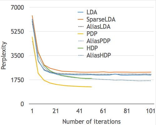
document d. From there the perplexity is then evaluated as: comes at no cost of degraded topic quality, as shown in
"D #−1 D Figure 6. The convergence speed and converged perplex-
X X ity of AliasLDA, AliasPDP, and AliasHDP almost perfectly
π(W|rest) := Nd log p(wd |rest) where match the non-alias counterparts. This further shows that
d=1 d=1
our choice of relatively small number of Metropolis-Hasting
nd k
Y X steps (2 per sample) is adequate.
p(wd |rest) = p(wi = w|zdi = t, rest)p(zdi = t|rest) The improved performance in running time of our alias
i=1 t=1
implementations can be seen in all phases of sampling when
Here we obtain the estimate of p(wi = w|zdi = t, rest) from compared to non-alias standard implementations (LDA,
the model being trained. To avoid effects due to variation in PDP, HDP). When compared to SparseLDA (Figure 3),
the number of topics, we hardcoded k = 1024 for all experi- the performance gain is salient during all phases on larger
ments except one (GPOL) where we vary k and observe the datasets (except for the early stage in Enron dataset), and
effect on speed per iteration. We use fixed values for hyper- the performance is very close on small datasets (0.35s per it-
parameters in all our models, setting α = β = 0.1 for LDA, eration on AliasLDA vs. 0.25s per iteration on SparseLDA).
a = 0.1, b = 10, and γ = 0.1 for the PDP, and b0 = b1 = 10, As the size of the data grows AliasLDA outperforms
γ = 0.1 for the HDP. For alias implementations, we fix the SparseLDA without degrading topic quality, reducing the
number of Metropolis-Hasting sampling steps at 2, as we amount of time for each Gibbs iteration on NYTimes corpus
observed a satisfactory acceptance rate (over 90%) at these by around 12% to 38% overall, on Enron corpus by around
settings. Only a negligible improvement in perplexity was 30% after 30 iterations, and on PubMedSmall corpus by
observed by raising this value. Furthermore, we did not ob- 27%-60% throughout the first 50 iterations. Compared to
serve degraded topic quality even when Metropolis-Hasting SparseLDA, the time required for each Gibbs iteration with
AliasLDA grows at a much slower rate, and the benefits of
2
Reuters Vol. 1, English language, 1996-08-20 to 1997-08-19 reduced sampling complexity is particularly clear when the
3
Source: www.cs.cmu.edu/˜enron average length of each document is small.34%, 37%, 41%, 43% respectively. In other words, it in-
creases with the amount of data, which conforms our in-
tuition that adding new documents increases the density of
ntw , thus slowing down the sparse sampler much more than
the alias sampler, since the latter only depends on kd rather
than kd + kw .
Perplexity vs. Runtime Perplexity vs. Iterations
GPOL
Figure 4: Comparison of SparseLDA and AliasLDA
Enron
on GPOL when varying the number of topics for
k ∈ {256, 1024, 2048, 4096}.
Seconds per iteration
Percentage of full PubMedSmall collection PubMedSmall
Figure 5: Average runtime per iteration when com-
pared on {10%, 20%, 40%, 75%, 100%} of the PubMedS-
mall dataset for SparseLDA and AliasLDA.
The gap in performance is especially large for more so-
phisticated language modelsl such as PDP and HDP. The
running time for each Gibbs iteration is reduced by 60% to
NYTimes
80% for PDP, and 80% to 95% for HDP, an order of magni-
tude on improvement.
5.5 Varying the number of topics
When the number of topics k increases, the running time
for an iteration of AliasLDA increases at a much lower
rate than SparseLDA, as seen from Figure 4 on dataset Figure 6: Perplexity as a function of runtime
GPOL since kd is almost constant. Even though the gap (left) and number of iterations (right) for LDA,
between SparseLDA and AliasLDA may seem insignificant SparseLDA, and LDA, PDP and HDP, both with
at k = 1024, it becomes very pronounced at k = 2048 and without using the Alias method. We see consid-
(45% improvement) and at k = 4096 (over 100%) This con- erable acceleration at unchanged perplexity.
firms the observation above that shorter documents benefits
more from AliasLDA in the sense that the average docu-
ments length L/D relative to the number of topics k be-
comes “shorter” as k increases. This yields a more sparse ndt 6. CONCLUSION
and lower kd for a document d on average. In this paper, we described an approach that effectively
reduces sampling complexity of topic models from O(k) to
5.6 Varying the corpus size O(kd ) in general, and from O(kw +kd ) (SparseLDA) to O(kd )
Figure 5 demonstrates how the gap in running time speed (AliasLDA) for LDA topic model. Empirically, we showed
scales with growing number of documents in the same do- that our approach scales better than existing state-of-the-
main. We measure the average runtime for the first 50 Gibbs art method when the number of topics and the number of
iterations on 10%, 20%, 40%, 75%, and 100% of PubMedS- documents become large. This enables many large scale ap-
mall dataset. The speedup ratio for each subset is at 31%, plications, and many existing applications which require ascalable distributed approach. In many industrial applica- [8] W. R. Gilks, S. Richardson, and D. J. Spiegelhalter.
tions where the number of tokens easily reaches billions, Markov Chain Monte Carlo in Practice. 1995.
these properties are crucial and often desirable in design- [9] T. Griffiths and M. Steyvers. Finding scientific topics.
ing a scalable and responsive service. We also demonstrated PNAS, 101:5228–5235, 2004.
an order of magnitude improvement when our approach is [10] G. Heinrich. Parameter estimation for text analysis.
applied to complex models such as PDP and HDP. With an Technical report, Fraunhofer IGD, 2004.
order of magnitude gain in speed, PDP and HDP may be- [11] M. Hoffman, D. M. Blei, C. Wang, and J. Paisley.
come much more appealing to many applications for their Stochastic variational inference. In ICML, 2012.
superior convergence performance, and more sophisticated [12] W. Li, D. Blei, and A. McCallum. Nonparametric
representation of topic distributions and language models. bayes pachinko allocation. In UAI, 2007.
For k = 1024 topics the number of tokens processed per
[13] G. Marsaglia, W. W. Tsang, and J. Wang. Fast
second in our implementation is beyond 1 million for all
generation of discrete random variables. Journal of
datasets except one (NYTimes), of which contains substan-
Statistical Software, 11(3):1–8, 2004.
tially more lengthy documents. This is substantially faster
than many known implementations when measured in num- [14] R. M. Neal. Markov chain sampling methods for
Dirichlet process mixture models. University of
ber of tokens processed per computing second per core, such
as YahooLDA [18], and GraphLab, given that we only utilise Toronto, Technical Report 9815, 1998.
a single thread on a single laptop CPU core. [15] J. Petterson, A. Smola, T. Caetano, W. Buntine, and
Acknowledgments: This work was supported in part by S. Narayanamurthy. Word features for latent dirichlet
a resource grant from amazon.com, a Faculty Research Grant allocation. In NIPS, pages 1921–1929, 2010.
from Google, and Intel. [16] J. Pitman and M. Yor. The two-parameter
poisson-dirichlet distribution derived from a stable
subordinator. A. of Probability, 25(2):855–900, 1997.
7. REFERENCES [17] I. Sato and H. Nakagawa. Topic models with
[1] K. Bache and M. Lichman. UCI machine learning power-law using Pitman-Yor process. In KDD, pages
repository, 2013. 673–682. ACM, 2010.
[2] D. Blei, T. Griffiths, and M. Jordan. The nested [18] A. J. Smola and S. Narayanamurthy. An architecture
chinese restaurant process and Bayesian for parallel topic models. In PVLDB, 2010.
nonparametric inference of topic hierarchies. Journal [19] Y. Teh, M. Jordan, M. Beal, and D. Blei. Hierarchical
of the ACM, 57(2):1–30, 2010. dirichlet processes. JASA, 101(576):1566–1581, 2006.
[3] D. Blei, A. Ng, and M. Jordan. Latent Dirichlet [20] A. J. Walker. An efficient method for generating
allocation. JMLR, 3:993–1022, Jan. 2003. discrete random variables with general distributions.
[4] W. Buntine and M. Hutter. A bayesian review of the ACM TOMS, 3(3):253–256, 1977.
poisson-dirichlet process, 2010. [21] C. Wang, J. Paisley, and D. M. Blei. Online
[5] C. Chen, W. Buntine, N. Ding, L. Xie, and L. Du. variational inference for the hierarchical Dirichlet
Differential topic models. In IEEE Pattern Analysis process. In Conference on Artificial Intelligence and
and Machine Intelligence, 2014. Statistics, 2011.
[6] C. Chen, L. Du, and W. Buntine. Sampling table [22] L. Yao, D. Mimno, and A. McCallum. Efficient
configurations for the hierarchical poisson-dirichlet methods for topic model inference on streaming
process. In ECML, pages 296–311, 2011. document collections. In KDD’09, 2009.
[7] J. Geweke and H. Tanizaki. Bayesian estimation of
state-space model using the metropolis-hastings
algorithm within gibbs sampling. Computational
Statistics and Data Analysis, 37(2):151–170, 2001.You can also read