Hydraulic transmissivity inferred from ice-sheet relaxation following Greenland supraglacial lake drainages - Nature
←
→
Page content transcription
If your browser does not render page correctly, please read the page content below
ARTICLE
                  https://doi.org/10.1038/s41467-021-24186-6                 OPEN

                  Hydraulic transmissivity inferred from ice-sheet
                  relaxation following Greenland supraglacial lake
                  drainages
                  Ching-Yao Lai 1,2,3 ✉, Laura A. Stevens                      2,4,   Danielle L. Chase5, Timothy T. Creyts2, Mark D. Behn6,
                  Sarah B. Das7 & Howard A. Stone 5
1234567890():,;

                  Surface meltwater reaching the base of the Greenland Ice Sheet transits through drainage
                  networks, modulating the flow of the ice sheet. Dye and gas-tracing studies conducted in the
                  western margin sector of the ice sheet have directly observed drainage efficiency to evolve
                  seasonally along the drainage pathway. However, the local evolution of drainage systems
                  further inland, where ice thicknesses exceed 1000 m, remains largely unknown. Here, we
                  infer drainage system transmissivity based on surface uplift relaxation following rapid lake
                  drainage events. Combining field observations of five lake drainage events with a mathe-
                  matical model and laboratory experiments, we show that the surface uplift decreases
                  exponentially with time, as the water in the blister formed beneath the drained lake
                  permeates through the subglacial drainage system. This deflation obeys a universal relaxation
                  law with a timescale that reveals hydraulic transmissivity and indicates a two-order-of-
                  magnitude increase in subglacial transmissivity (from 0.8 ± 0.3 mm3 to 215 ± 90.2 mm3 ) as
                  the melt season progresses, suggesting significant changes in basal hydrology beneath the
                  lakes driven by seasonal meltwater input.

                  1 Department  of Geosciences, Princeton University, Princeton, NJ, USA. 2 Lamont-Doherty Earth Observatory, Columbia University, Palisades, NY, USA.
                  3 Program in Atmospheric and Oceanic Sciences, Princeton University, Princeton, NJ, USA. 4 Department of Earth Sciences, University of Oxford, Oxford, UK.
                  5 Department of Mechanical and Aerospace Engineering, Princeton University, Princeton, NJ, USA. 6 Department of Earth and Environmental Sciences, Boston

                  College, Chestnut Hill, MA, USA. 7 Department of Geology and Geophysics, Woods Hole Oceanographic Institution, Woods Hole, MA, USA.
                  ✉email: cylai@princeton.edu

                  NATURE COMMUNICATIONS | (2021)12:3955 | https://doi.org/10.1038/s41467-021-24186-6 | www.nature.com/naturecommunications                                1
ARTICLE                                                                  NATURE COMMUNICATIONS | https://doi.org/10.1038/s41467-021-24186-6

T
         housands of supraglacial lakes form annually on the sur-             the time at which uplift begins to relax continuously back to pre-
         face of the Greenland Ice Sheet in response to seasonal              drainage values. Longer relaxation times t rel are generally
         melt that fills topographic depressions. Many of these lakes          observed for drainages that occur earlier in the melt season
drain rapidly ( 1000 m above sea level [a.           August10. Subglacial hydrological models indicate that short,
s.l.])13,14, where evolution of local basal hydrology remains poorly          discontinuous channels form following lake drainage, but the
constrained by observations. Furthermore, observational-based                 discharge from the channel is small compared to the discharge
estimates for hydraulic transmissivity, a key parameter control-              through the distributed sheet13. In reality, either a purely
ling the water discharge in a subglacial sheet for a given hydraulic          distributed system without any channels or a channelized system
potential gradient, are scarce. Here we calculate the local                   dominated by turbulent discharge are unlikely end members of
hydraulic transmissivity9,15 beneath rapidly draining supraglacial            the subglacial drainage system beneath the lakes. Therefore,
lakes (1000–1350 m a.s.l.) at their time of drainage using a                  instead of quantifying the efficiency of a purely distributed sheet
combination of field observations, a mathematical model, and                   or a purely turbulent channel, here we use transmissivity to
laboratory experiments in order to quantify the seasonal changes              characterize the bulk subglacial drainage system (valid within 2–6
of local hydraulic transmissivity driven by seasonal meltwater                km horizontal distance from the lake, as explained below), where
inputs.                                                                       a wide range of drainage features likely co-exist (e.g., distributed
                                                                              flows through porous sediment sheets17, thin films18–20 linked
Results                                                                       cavities21,22, localized flows through channels, and weakly
Relaxation of surface uplift following lake drainage. The rapid               connected systems23). A similar approach was developed by
drainage of lakes injects surface meltwater into the ice–bed                  Sommers et al. 24. Because the horizontal extent of the water flow
interface. The water can be transiently stored in water-filled                 (~kilometers) is much larger than the vertical extent (~meters),
“blisters” (Fig. 1a) that lift and deform the overlying ice                   the bulk subglacial drainage system is treated as a continuum
sheet2,3,6,16. After a lake drainage event, surface uplift decays over        water sheet of effective depth h0 , effective permeability k, and
time1 as water exits the blister and spreads along the ice–bed                porosity ϕ (ratio between water-filled space to total space).
interface (Fig. 1b). Previous studies have documented the                        Uplift relaxation is driven by the elastic deformation of ice
initial stages of lake drainage and blister formation1,2 and mod-             lying above the water-filled blister and resisted by the viscous
eled the effect of lake drainage on the subglacial hydrological               dissipation of the water flow in the distributed drainage system.
system13. Here we focus on the long-term surface relaxation                   Below we use scaling arguments to obtain a characteristic
(1–10 days) of the ice sheet after a lake drains to quantify the              timescale of blister relaxation t c . The full mathematical model
hydraulic transmissivity9,15 of the surrounding subglacial drai-              for blister relaxation dynamics is detailed in Supplementary
nage system.                                                                  Information Section 1.
   Using ice-sheet surface elevation data from on-ice GPS                        For a blister of maximum thickness H and radius R (Fig. 2a)
stations, we characterize the relaxation timescale for five lake               the blister volume scales as V  2παHR2 (equation (S.15)),
drainage events that occurred between 2006 and 2012 at three                  where α is a dimensionless parameter related to the shape of the
separate lakes located up to ~200 km apart along the western                  blister. From mass conservation, the blister volume relaxation
margin of the Greenland Ice Sheet (Fig. 1d–h; Supplementary                   rate ðdV=dt  V=t c Þ equals the water flux entering the subglacial
Table 1). The five rapid lake drainages have drainage dates that               water sheet with flow velocity up (red arrows in Fig. 2a) at radial
span from the early melt season (typically May through June)                  distance r. Thus, a mass balance yields (see equations (S.12)
through the mid-melt season (typically July through August). We               and (S.15))
find a wide range of relaxation timescales of surface uplift (from
12 h to 10 days) depending on when lake drainage occurs within                                         V 2παHR2
                                                                                                                rϕup h0                      ð1Þ
the melt season (Fig. 1d–h). Ice-sheet surface uplift relaxation is                                    tc   tc
fitted by an exponential function (dashed curves in Fig. 1d–h and
Supplementary Fig. 4f–j) to quantify the relaxation time t rel . The            The flow in the bulk subglacial water sheet can be described by
two uplift peaks following the 2011 drainage shown in Fig. 1e                 Darcy’s law for flow in porous materials17–22, where the water
likely result from additional water injection into the blister from           flux ϕup (volume per time per unit area crossing the flow)
nearby surface or basal sources (Methods). We set time zero to be             increases linearly with the gradient of water pressure p. Assuming

2                 NATURE COMMUNICATIONS | (2021)12:3955 | https://doi.org/10.1038/s41467-021-24186-6 | www.nature.com/naturecommunications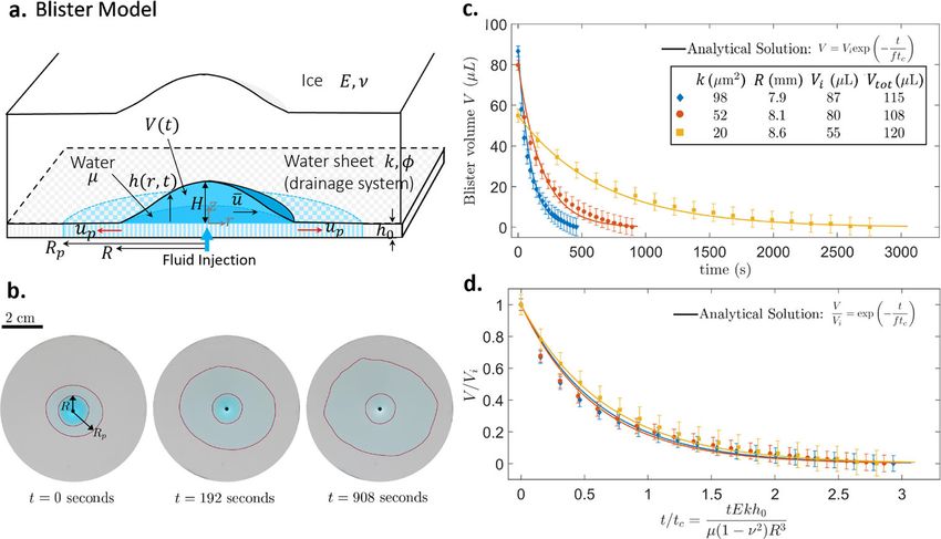
NATURE COMMUNICATIONS | https://doi.org/10.1038/s41467-021-24186-6                                                                               ARTICLE

Fig. 1 Ice-sheet uplift relaxation following rapid supraglacial lake drainage. Schematic drawings of the North Lake GPS array that reports ice-sheet
surface uplift and speed (a) during subglacial blister formation at the time of rapid drainage, and (b) post-drainage relaxation as the blister drains into the
surrounding ice-bed interface. c The locations of North Lake (NL), South Lake (SL), and Lake F (LF) are marked by the blue dots. d–h Ice-sheet surface
elevation during rapid drainage (drainage start time marked by arrows) and post-drainage uplift relaxation from GPS stations for five different drainages,
where post-drainage uplift relaxation begins at time = 0 days. Dashed curves show vertical displacement data fit to the exponential function,
hðtÞ ¼ hi expðt=trel Þ. The fitted trel , the lake drainage year, and the station name for each GPS station are listed in the table. For the 2011 data, we therefore
set time zero to be the time after which uplift only relaxes, and no significant amounts of additional water enter the blister (Mathods).

the discharge in channels are negligibly small compared with that                  sheet over r > R and considering mass conservation, we obtain a
of the bulk subglacial system13, Darcy’s law holds to the first                     horizontal pressure drop (equation (S.18)) of magnitude.
order. Thus, the bulk subglacial flow obeys Darcy’s law
                                                                                                                         μ V Rp
ϕup ¼  μk ∇p, where μ is water viscosity. Note that in both field                                               Δpv             lnð Þ                          ð2Þ
                                                                                                                        h0 k t c    R
data and our laboratory experiments the blister radius R remains
unchanged during blister relaxation (Fig. 2b) and is assumed                       where Rp is the radius of the invading water front in the
constant in our model. We estimate that the horizontal viscous                     water sheet.
pressure drops in the water sheet and the blister for r < R are                       Deformation of the ice overlying the blister generates elastic
negligibly small (Supplementary Information Section 1.5) com-                      stresses in the ice sheet. For a penny-shaped blister3,25–27, the
pared with the viscous pressure drop Δpv in the water sheet at                     magnitude of the elastic stresses in ice can be estimated by
r > R. Integrating the pressure gradient radially along the water                  Hooke’s law corresponding to an approximate strain H=R

NATURE COMMUNICATIONS | (2021)12:3955 | https://doi.org/10.1038/s41467-021-24186-6 | www.nature.com/naturecommunications                                          3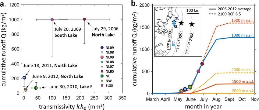
ARTICLE NATURE COMMUNICATIONS | https://doi.org/10.1038/s41467-021-24186-6
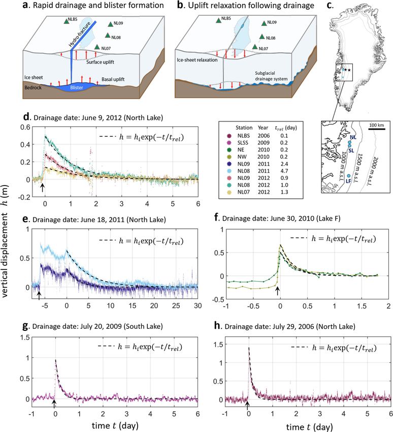
Fig. 2 Experimental validation of the mathematical model. a Schematic of the blister model. An elastic layer (ice) with Young’s modulus E and thickness d
over a porous substrate (drainage system) of thickness h0 , porosity ϕ, and permeability k: Injection of a liquid with volume V tot and viscosity into the
interface between the elastic layer and the substrate forms a blister. The experimental parameters are listed in Table 1 and the uncertainties are listed in
Supplementary Table 3. b The top view of the experimental relaxation dynamics, during which liquid in the blister (dark blue) enters the pore space (light
blue), increasing fluid area in the porous substrate. The blister and the fluid front in the porous substrate are outlined. During relaxation the blister radius R
remains approximately constant. c Measured blister volumes VðtÞ for three different substrate permeabilities decrease exponentially with time. The
analytical solution is given by Eq. (6). d The dimensionless experimental data fall onto a common curve, agreeing well with the exponential solution (Eq. (6)
with f ¼ 0:6 0:7 (Table 1); solid curves).
(see equation (S.16)): ordinary differential equation for the blister volume VðtÞ:
EH E V μ V tot V dV
Δpe ð3Þ þ ln ¼0 ð5Þ
2ð1 ν 2 ÞR 1ð1 ν 2 Þ 2απR3 4πh0 k ϕπh0 R2 dt
For a typical blister radius R 2 km and maximum thickness where V tot is the total volume of water in the system. Eq. (5) can
H 1 m, and ice with Young’s modulus E 10 GPa and be approximated by a linear ordinary differential equation
Poisson’s ratio ν 0.3, the elastic stress is Δpe 2 MPa. The (Supplementary Information Section 1.4; equation (S.25)),
elastic stresses caused by the blister are balanced by an increase in yielding exponential solutions for the blister volume VðtÞ and
water pressure in addition to the hydraulic potential. Thus, the thickness hðr; tÞ as a function of time t and radial distance r:
water pressure in the blister at the base of a uniform ice sheet of
thickness d 1 km is p ¼ ρi gd þ ρw gh þ Δpe (equation (S.38)), t
VðtÞ ¼ V i exp ð6Þ
where hðr; tÞ is the water thickness in the blister, ρw and ρi are the ft c
water and ice density, respectively, and g is the gravitational
acceleration. Subglacial flow is driven by the water pressure
gradient ∇p, where the gradient of ice and water overburden t
hðr; tÞ ¼ hi ðrÞexp ð7Þ
pressure are negligible compared with that of the elastic stress ft c
(Supplementary Information Section 2). Thus, during ice-sheet
relaxation the elastic stresses, rather than the ice and water where V i ¼ Vðt ¼ 0Þ, hi ðrÞ ¼ hðr; t ¼ 0Þ, and f is a numerical
overburden pressure, dominantly drive subglacial flow and blister pre-factor (equation (S26)). Comparing Eq. (7) with hðtÞ ¼
relaxation. hi expðt=t rel Þ gives f ¼ t rel =t c : The analytic approximation is in
The relaxation dynamics are governed by a balance close agreement to the numerical solution (Supplementary Fig. 1).
between the elastic stresses Δpe driving the relaxation and the The relaxation dynamics are negligibly impacted by the bed slope
pressure drop Δpv resisting the subglacial flow, i.e., Δpe Δpv . (Supplementary Information Section 2) and the melting and
Thus, Eqs. (1–3) give the characteristic relaxation time viscous motion of ice (Supplementary Information Section 3).
t c ¼ 4παlnðRp =RÞμR3 ð1 ν 2 Þ=ðEkh0 Þ. Neglecting the constants Based on field observations and lab experiments, we assume R
is constant so that the only way for blister volume to decrease is
of magnitude
R order one (e.g., π) and the numerical pre-factor
by pushing water through the porous water sheet, yielding an
αln R f ¼ Oð1Þ (equation (S.26)) that do not affect the
p
exponential decay of blister height. In contrast, Hewitt et al.16
scaling, we obtain the characteristic relaxation time: considered a blister propagating on a water-filled porous sheet
with an increasing R and decreasing h. In their model, water
t c ¼ μR3 ð1 ν 2 Þ=ðEkh0 Þ ð4Þ volume in the blister V is constant and does not leak into the
porous water sheet, resulting in a power-law decrease of blister
This timescale will be used to rescale the experimental and height as a function of time16. A comparison of the GPS uplift
field data. data with the power-law decay16 and our exponential decay (Eq.
Considering mass conservation and a force balance analysis (7)) is shown in Supplementary Fig. 7. The GPS uplift data
(Supplementary Information Section 1), we obtain a nonlinear exhibits better agreements with our exponential solutions.
4 NATURE COMMUNICATIONS | (2021)12:3955 | https://doi.org/10.1038/s41467-021-24186-6 | www.nature.com/naturecommunicationsNATURE COMMUNICATIONS | https://doi.org/10.1038/s41467-021-24186-6 ARTICLE
Laboratory experiments. Next, we tested the analytic model (Eqs.
that the dimensionless parameters (B; C) of the experiments match that of the field data, meaning experiments fall into the same physical regimes as the field observations. Derivations of the governing equation and the non-dimensionalization are detailed in Supporting
Although the dimensional governing equation (equation (S.21)) depends on nine dimensional parameters (ϕ; h0 ; k; E; ν; μ; V tot ; V i ; R), its dimensionless form (equation (S.23)) only depends on two dimensionless parameters (B; C). We designed the experimental parameters so
Numerical factors
(4) and (6)) against our laboratory experiments, which allow
0.70
0.70
0.48
0.48
0.48
0.79
0.58
0.67
0.75
0.61
0.61
0.61
precise control and direct measurement of sheet permeability.
f
Experiments on fluid peeling between an elastic sheet and a non-
permeable rigid substrate have previously been investigated28. In
0.32
0.32
contrast, here we consider a porous substrate that mimics the
drainage system. In our experiment, a fluid-filled blister (dark
α
blue in Fig. 2b) is generated via liquid injection into the interface
between a transparent elastic layer and a porous substrate. This
0.04
0.06
0.06
0.08
0.08
0.05
0.10
0.19
0.12
0.11
0.11
0.11
setup mimics ice lying above the drainage system (Fig. 2a). After
C
injection of liquid, the fluid permeates from the blister through
Dimensionless parameters
the porous substrate (light blue in Fig. 2b), the blister thickness
decreases and the blister radius remains unchanged (Supple-
2.18
1.32
1.35
1.14
Information. Numerical factor α 0:32 was found empirically by fitting all experimental data to Eq. (6). When calculating C for the field data, we assumed the thickness of the water sheet h0 is on the order of 0.1 m13.
B
mentary Movie 1), which differs from the increasing R in Hewitt
et al. (2018)16. Our lab experiments show that varying the per-
meability of the porous substrate k significantly impacts the
8.4 × 10⁻⁷
4.7 × 10⁻⁸
9.3 × 10⁻⁸
2.2 × 10⁻⁶
2.2 × 10⁻³
1.5 × 10⁻⁶
1.2 × 10⁻⁶
1.6 × 10⁻³
1.3 × 10⁻³
1.1 × 10⁻⁶
1.1 × 10⁻⁶
1.1 × 10⁻⁶
relaxation timescale in the experiments (Fig. 2c). The blister
volume VðtÞ relaxes exponentially with time, validating our
A
analytical solution (Eq.(6), curves in Fig. 2c). All parameters in
the analytical solution can be calculated based on the experi-
mental variables except for the pre-factor f (Table 1). Since t c /
8.6 mm
7.9 mm
8.1 mm
2.4 km
2.4 km
2.9 km
2.2 km
2.2 km
2.2 km
3.2 km
1.8 km
1.8 km
R3 via Eq.(4), the relaxation time (~103 seconds) of a laboratory-
scale blister (R~10 mm) is expected to be much shorter than that
R
observed in the field. After rescaling the blister volume V with V i
and time t with t c (Eq.(4)), the experimental data for different
0.007 km3
0.040 km3
0.007 km3
0.007 km3
0.007 km3
0.007 km3
0.027 km3
0.016 km3
permeabilities collapse onto a universal curve (Fig. 2d), demon-
0.016 km3
strating the model’s success in predicting the impact of perme-
Blister
80 μL
87 μL
55 μL
ability on the relaxation timescale. Here the thickness d of the
overlying elastic layer is roughly the same as the blister radius R, Vi
similar to field observations. When d R the relaxation time-
scale obeys a different scaling29.
0.008 km3
0.008 km3
0.008 km3
0.008 km3
0.008 km3
0.044 km3
0.030 km3
0.018 km3
0.018 km3
108 μL
120 μL
115 μL
Inferring hydraulic transmissivity from surface GPS data. We
V tot
then applied the validated model to estimate hydraulic trans-
missivity kh0 15 of the subglacial water sheet from surface uplift
data following the five lake drainage events (Supplementary
1 mPas (water)
Table 1). The relaxation time t rel of each set of GPS data was
obtained by fitting hðtÞ ¼ hi expðt=t rel Þ (dashed curves in Fig. 1)
0.8 Pa·s
to the GPS data. According to Eq.(4) and f ¼ t rel =t c , the
Liquid
hydraulic transmissivity can be expressed as kh0 ¼ μR ð1ν Þ
3 2
¼
μ
Et c
f μR Etð1ν Þ (lines in Fig. 3a) and calculated using the relaxation
3 2
rel
time t rel , the Young’s modulus of ice E, water viscosity μ, Pois-
0.5
0.3
Table 1 Parameters and their definitions used in this study.
son’s ratio ν, blister radius R estimated from the lake volume V tot
ν
(Methods), and the pre-factor f ¼ Oð1Þ (equation (S.26);
Porous sheet properties: ϕ :porosity, h0 : thickness, k: permeability, kh0 : transmissivity
C Þ; where γ e 0:63
Table 1). This transmissivity estimate is valid within a 2–6 km
1 km
1 cm
horizontal distance (the extent of water in the sheet displaced by
e1
d
Elastic layer properties: E: Young’s modulus, d: thickness, ν: Poisson’s ratio
the lake volume) from the lake-drainage location. The transmis-
Elastic layer
sivity estimated for each lake drainage event based on the GPS
217 kPa
10 GPa
uplift data is shown in Fig. 3a and Table 1. Note that the varia-
bility of the transmissivity estimated from different stations for
Dimensionless parameters: A 16π VR3 kh0 ;B VVtot ;C ϕπhV0 R ;fαlnð Bγ
E
the same drainage event is less than that between different drai-
Liquid: μ: viscosity, V tot : volume of total injected liquid
nage events. The uncertainties propagated in the transmissivity
2
i
estimate are reported in Supplementary Table 2 (Methods). The
20 × 90 μm3
98 × 90 μm3
52 × 90 μm3
100.0 mm3
215.0 mm3
44.0 mm3
43.0 mm3
changes in transmissivity kh0 could be caused by the evolution of
0.8 mm3
4.5 mm3
6.2 mm3
5.7 mm3
1.7 mm3
i
kρ g
not only the effective permeability k (or conductivity K μw 30)
kh0
Porous sheet
3 6
but also effective thickness h0 of the bulk subglacial drainage
i
Blister: R: radius, V i : initial volume
system.
Definitions of parameters:
0.5
0.5
ϕ
Universal uplift relaxation dynamics. To demonstrate the uni-
versality of the time-dependent uplift relaxation data, we rescaled
the surface uplift data (Fig. 3b) by the characteristic relaxation
Field data
Lab exp.
time t c , as calculated from Eq. (4) using the parameters listed in
Fig. 3a, and the initial vertical displacement hi . The rescaled data
collapse (Fig. 3c) onto the analytical solution, Eq. (7) Thus,
NATURE COMMUNICATIONS | (2021)12:3955 | https://doi.org/10.1038/s41467-021-24186-6 | www.nature.com/naturecommunications 5ARTICLE NATURE COMMUNICATIONS | https://doi.org/10.1038/s41467-021-24186-6
Fig. 3 Hydraulic transmissivity and the universal dynamics of uplift relaxation. a The relaxation time trel obtained from surface uplift data from different
stations and the predicted hydraulic transmissivity kh0 . Detailed information for each data set is shown in the table. Here the supraglacial lake volume is
assumed to be the total volume V tot injected into the blister and the water sheet. The black lines (trel ¼ f μR ð1ν Þ
3 2
E ðkh0 Þ1 ) are the model predictions for
different blister radii R. The lake volume V tot of Lake F and North Lake listed in the table are taken from references 6 and the lake volume of South Lake is
1, 2,
estimated in the Methods. Surface uplift data from five drainages of three different lakes as recorded by seven different GPS stations are plotted in (b)
dimensional and (c) dimensionless forms. Despite a wide range of relaxation times, when rescaled by the characteristic relaxation time tc (Eq. (4)) and
initial vertical displacement hi , all field uplift data collapse onto the exponential analytical solution (Eq. (7), red dashed line (c) with f ¼ 0:6 averaged over
all datasets (Methods)). Upper and lower dashed lines represent the solutions with the highest and lowest f (Table 1), respectively, among all the data sets.
despite variability in local lake basin and ice-sheet bed geometry, 29 (2006 drainage) as the cumulative surface melt volume differs
surface uplift magnitude, and timescale of uplift relaxation, the by a factor of 25 (Fig. 4a). The seasonal change of hydraulic
collapse of the data onto a universal curve indicates that the conductivity is important for reconciling mismatch between
relaxation dynamics depends to first order on two dimensionless modeled and observed subglacial water pressure32. Downs et al
parameters, h=hi and t=t c . Notably, both the dimensionless field (2018)32 included a simple linear relationship between melt input
data (Fig. 3c) and dimensionless experimental data (Fig. 2d) fall and hydraulic conductivity in a subglacial hydrological model and
onto the exponential solution (Eqs. (6–7)), demonstrating the found an improved match between the modeled subglacial water
universality of the uplift relaxation dynamics. pressure with borehole observations in the late melt season. Our
work provides observational evidence of the seasonal changes of
hydraulic transmissivity. Note that our result does not imply that
Seasonal changes of transmissivity under supraglacial lakes. transmissivity solely depends on cumulative surface runoff. The
Finally, we compare the transmissivities for lakes draining during processes controlling the shift in transmissivity are left for future
the early- and mid-melt season. Our results suggest the local studies. Comparing the range of transmissivity values we obtained
transmissivity of the basal drainage system beneath North Lake from the field data (kh0 ¼ Oð1 102 Þ mm3) with the hydraulic
can change by up to two orders of magnitude between early June conductivity used in large-scale hydrological models13
and late July. Early-season events relax more slowly as char- (K μw 0:05 0:5 m s−1), we calculate that the sheet depth
kρ g
acterized by a low-transmissivity drainage system (kh0 ¼ Oð1Þ
mm3). By contrast, the mid-season events relax faster and are best is of order h0 ¼ O 102 101 m. All parameters used in the
explained by high transmissivity (kh0 ¼ Oð102 Þ mm3). When transmissivity calculation are listed in Table 1.
comparing our estimates of hydraulic transmissivity to modeled
cumulative surface runoff31 at the time of lake drainage, we Discussion
observe that transmissivity generally increases with increased We infer that local hydraulic transmissivity under North Lake
cumulative runoff (Fig. 4a). Our results suggest that local trans- (~1000 m a.s.l.) likely changes seasonally. Our method can be
missivity beneath North Lake at ~1000 m a.s.l. differs by up to applied to estimate local transmissivity beneath other draining
two orders of magnitude between June 9 (2012 drainage) and July supraglacial lakes simply based on surface observation of uplift
6 NATURE COMMUNICATIONS | (2021)12:3955 | https://doi.org/10.1038/s41467-021-24186-6 | www.nature.com/naturecommunicationsNATURE COMMUNICATIONS | https://doi.org/10.1038/s41467-021-24186-6 ARTICLE
Fig. 4 Seasonal variation of hydraulic transmissivity. a Transmissivity inferred from five drainage events across three lakes and the corresponding
cumulative runoff at the lake drainage time. Cumulative runoff is the sum of daily, 11-km resolution RACMO runoff estimates31 from the first day of the year
up to the drainage date at the nearest RACMO grid cell to the drainage location (Methods). Vertical error bars (Methods) show the difference in
cumulative runoff estimates between RACMO31 and MAR34 runoff estimates. b Time evolution of cumulative runoff (monthly output) obtained from the
regional climate model MAR averaged from 2006 to 2012 (solid curves) and its 2100-projections under the RCP 8.5 scenario34 (dashed curves), evaluated
at the three locations (elevations) marked as stars on the inset map (same map as the inset in Fig. 1c). The star at 1000 m a.s.l. is the North Lake location.
The labels mark the day of year (DOY) of the drainage events and the corresponding 2006-2012 averaged cumulative runoff.
and lake volume. Dye and gas tracer experiments10 have the all sectors of the ice sheet to constrain processes governing the
advantage of tracking subglacial water speed at different times of present and future evolution of sliding in the ice-sheet interior.
the year, which well characterize the evolution of subglacial effi-
ciency near the marginal areas. To extend these experiments to Methods
higher-elevation regions (>1000 m a.s.l.; far away from the ice- GPS data. For the 2006, 2011, and 2012 North Lake and 2009 South Lake drainage
sheet margin), however, the measured water velocity must be events, continuous 30-s resolution GPS data collected by dual-frequency Trimble
averaged along the entire tracer pathway (e.g., the tracing NetR9 receivers were processed with Track software38, following the methodology
experiment performed at moulin L41 by Chandler et al. (2013)10 previously presented for the same GPS data in Stevens et al. 2 and Stevens et al. 39.
GPS data for each station were processed individually relative to the 30-s resolution
gives a water velocity averaged along a 41-km-long water path- Greenland GPS Network (GNET) KAGA base station located on bedrock, 55 km
way). Thus, it is unclear to what extent the drainage system from North Lake40. 1-σ error output from Track software for these data are the
evolves locally in higher elevation regions from dye and gas tracer order of ± 2 cm in the horizontal and ± 5 cm in the vertical across all stations and
experiments. Our results imply that the drainage system likely years2. GPS data are archived at UNAVCO (see Data and materials availability).
evolves locally at the lake elevations (~1000 m a.s.l.). In addition,
tracer experiments are limited to sampling moulins in land- Uplift data processing. The vertical displacement of each GPS station shows
terminating glaciers located mainly in south-west Greenland. By trends related to background ice sheet advection through the lake basins. For
example, in Supplementary Fig. 4a–e the background vertical displacement yðtÞ
contrast, supraglacial lakes are widespread over the ice sheet and slowly varies with time t before and after the uplift peak caused by the 5 lake
are forming in progressively higher elevation regions as the cli- drainage events. These background trends are fitted to a linear model (y ¼ at þ b,
mate warms33. where a; b are constants) and subtracted to yield the detrended vertical displace-
Quantifying hydraulic transmissivity of high-elevation areas ment hðtÞ (Supplementary Fig. 4f–j, also plotted in Fig. 1d–h). When fitting the
relative vertical displacement to the linear model, we avoid the peak caused by lake
(>1000 m a.s.l.) is crucial for understanding ice-sheet behavior in drainage. For consistency, we fit the linear model to the relative vertical dis-
a warming climate. Our method provides an approach to deter- placement data, terminating at time t end (the right end of each plot in Supple-
mine the magnitude of transmissivity of high-elevation regions mentary Fig. 4), after the peak during t end =2ARTICLE NATURE COMMUNICATIONS | https://doi.org/10.1038/s41467-021-24186-6
displacements and lake drainage volumes have not been previously detailed for (estimated blister radii are listed in the table in Fig. 3) and the uncertainty asso-
South Lake (68.57˚ N, 49.37˚ W) (Supplementary Fig. 5a). South Lake is located at ciated with blister radius estimates is related to the uncertainties in estimating V tot
1050 m a.s.l. on the western margin of the Greenland Ice Sheet, roughly 22 km and hmax (5th column in Supplementary Table 2).
south of North Lake41,42.
In 2009, South Lake rapidly drained on July 20, 2009, as indicated by uplift of Hydraulic transmissivity. Finally, the errors associated with estimating the trans-
GPS station SLSS (Supplementary Fig. 6b). No additional GPS were deployed in the missivity kh0 (last column in Supplementary Table 2) is propagated from errors in
vicinity of South Lake with a temporal sampling resolution adequate to observe the V tot ; hmax , and R. The error bar in kh0 varies from 20% for the 2011 and 2012
rapid drainage event in 2009. Ice-sheet vertical and horizontal displacements drainage events to 40-50% for the 2006 and 2009 drainage events, due to larger
following the 2009 drainage of South Lake are most similar to the 2006 rapid uncertainties in both measuring lake volume and estimating maximum blister
drainage of North Lake (Supplementary Fig. 6a). SLSS station attains an uplift of height.
0.93 m over the initial 1.2 h of the drainage event, before relaxing to its pre-
drainage elevation over the following 14 h (Supplementary Fig. 6b). SLSS depicts
Numerical pre-factor f . One benefit of dimensionless solutions is that the shape of
a pre-drainage along-flow velocity of 141.7 m yr−1, and a duration of 2.05 days is
uplift data hðtÞ for a range of V tot and kh0 can be compared with the theory on a
observed between the time of lake drainage and the time of along-flow
dimensionless h=hi t=t c plot (Fig. 3c). Theoretically we expect a slight spread of
displacement attaining the displacement predicted by pre-drainage along-flow
dimensionless data on Fig. 3c because the analytical solution of blister height (red
velocities (Supplementary Fig. 6b).
curve in Fig. 3c; Eq. (7)) depends not only on h=hi and t=t c but also f ¼
The 30-m resolution MEaSUREs Greenland Ice Mapping Project (GIMP)
αln½ðB γÞ=C (equation (S.26)). We estimate that f varies between individual
Digital Elevation Model (DEM) from GeoEye and WorldView Imagery, Version
43,44 drainage events in the range f ¼ 0:5 0:8, as shown in the last column in Table 1.
1 and Landsat 7 imagery were used to estimate the pre-drainage volume of
In Fig. 3c we plot the solution using the value f ¼ 0:6 averaged over all datasets
South Lake. The last available image of South Lake in 2009 was taken on July 15,
(red dashed curve). The upper and lower bounds of the solutions calculated using
2009, five days prior to South Lake’s rapid drainage (Supplementary Fig. 5a). The
f ¼ 0:5 and f ¼ 0:8, respectively, are illustrated by the black dashed lines in Fig. 3c.
lake margin on July 15, 2009 was mapped (Supplementary Fig. 5a) and used to
compare to elevation contours of South Lake from the GIMP DEM
(Supplementary Fig. 5b). The region of the GIMP DEM covering South Lake was Systematic errors. There are two constants that can cause systematic uncertainties:
created with a WorldView image taken on July 17, 201243, at which time South the Young’s modulus of ice (E 1010 Pa) and the volume ratio between the lake
Lake basin did not host a lake, as South Lake drained on or before June 12, 2012 volume and the initial blister volume (B V tot =V i 1:14), estimated from the
based on the Landsat image archive. Therefore, while there could be elevation 2012 North Lake volume and the NIF-calculated initial blister volume. Since they
changes between 2009 and 2012, the GIMP DEM over South Lake depicts a dry cause systematic errors, variations in these parameters will not affect the collapse of
lake basin. the data in Fig. 3c, but will systematically shift the transmissivity value. If we
Based on a comparison between the mapped South Lake margin and GIMP consider an extreme parameter range, E ¼ Oð109 1010 Þ Pa and B ¼ 1 5, the
DEM elevation contours, the South Lake margin elevation was estimated to be transmissivity kh0 / R3 =E / B3=2 E1 will be systematically multiplied by a factor
1050.5 m a.s.l. (Supplementary Fig. 5b), yielding a lower bound on the lake volume in the range of 0.1 ~ 12.
estimate for South Lake of 0.029 km3, with maximum lake depths on the order of
10–15 m (Supplementary Fig. 5c). The GIMP DEM reports a 1σ error of ±1.27 m
Transmissivity versus surface cumulative runoff. The change of basal trans-
for every elevation estimate in the South Lake area (Supplementary Fig. 5b). A ± 1σ
missivity between the early and mid-melt season is demonstrated in Fig. 4a. The x-
error on the estimated lake margin elevation of 1050.5 m a.s.l. (Supplementary
axis is the transmissivity inferred from the five drainage events in 2006, 2009, 2010,
Fig. 5b) yields a lake volume error of 0.006 km3. This error estimate should
2011, and 2012 for the three lakes. The y-axis is the cumulative runoff from the first
presumably be a bit larger (0.01 km3), given the GIMP DEM time stamp is in
day of the year in which runoff occurs through the drainage date. The cumulative
2012, and the last pre-drainage image of South Lake was taken 4 days before the
runoff shown by the y-position of the symbols in Fig. 4a is calculated from daily 11-
2009 drainage. Following this methodology, we estimate the 2009 South Lake
km resolution RACMO runoff estimates31 over the 11-km grid cell at locations of
drainage volume to be 0.03 ± 0.01 km3.
the GPS stations. The Lake F location is 67.01˚ N 48.74˚ W6.
The difference in cumulative runoff estimates between RACMO31 and MAR34
Uncertainties in Estimating Model Parameters. The error bars of transmissivity in late July is large and reflected in the vertical error bars. The error bars of the
kh0 in Fig. 3a result from uncertainties in estimating (1) lake volume V tot , (2) cumulative runoff in Fig. 4a cover the range of values extrapolated from the
maximum blister height at the beginning of lake drainage hmax , and (3) blister regional climate MAR34 (v3.5.2) model’s monthly output averaged from 2006 to
radius R. The uncertainties associated with the three parameters are listed in 2012 (y-positions of the symbols on the solid blue curve in Fig. 4b).
Supplementary Table 2 and detailed below.
Additional surface water injection near North Lake. The minor uplift peaks
Lake volume. The lake volume V tot and its measurement errors for 2009 North observed at NL08 and NL09 ~6 days after the 2011 North Lake drainage could be
Lake, 2010 Lake F, 2011 and 2012 North Lake are reported in Das et al.1, Doyle related to additional water injected to the bed from basal or surface sources. The
et al.6, Stevens et al.2, respectively. The estimated uncertainty for 2006 South Lake second uplift peak occurred on 2011/175 (day of year (DOY) 175 in 2011), roughly
volume is detailed in Methods. The lake volume values are listed in the table in 6 days after the initial uplift peak on 2011/169. There are three LandSat-7 images
Fig. 3 with error bars listed in Supplementary Table 2. available over this time window (Supplementary Fig. 8). From 2011/168 to 2011/
170 (Supplementary Fig. 8a, b), North Lake is the only supraglacial feature to drain
Maximum blister height. The maximum blister height hmax for all drainage events from view. Next, there is a 7-day gap in images with the next available LandSat-7
are listed in the table in Fig. 3 with uncertainties listed in Supplementary Table 2. image on 2011/177 (Supplementary Fig. 8c). This image shows the drainage of two
For 2011 and 2012 drainage events, hmax are available from the Network Inversion lakes immediately to the northwest of the northern extent of the GPS array. It is
Filter (NIF)45 algorithm in Stevens et al. (2015)2, which solves for the blister height difficult to diagnose the drainage date and drainage style based on the images, but
based on surface displacement data from a network of 15 GPS stations around the the regional bed topography (Supplementary Fig. 2b) suggests that water drained to
blister at North Lake. We would expect the uncertainties in hmax from NIF output the bed from these lakes could then flow beneath North Lake to avoid the basal
to be on the order of magnitude of the uncertainties in the GPS elevation data ridge to the northwest. Based on this temporally sparse LandSat-7 imagery, two
(±0.05 m). The NIF calculation is not performed for 2006, 2009, and 2010 drainage supraglacial lakes located 1–2 km from the northern extent of the GPS array are
events because there are not enough nearby GPS stations available to build an observed to drain within 1–8 days following the 2011 North Lake drainage (2011/
adequate network for the inversion, so hmax is estimated by assuming that both (1) 169).
the initial blister shape [i.e., height to radius ratio (Ar hmax =R ¼ Oð103 Þ) and
(2) the ratio of total water volume injected into the ice-bed interface (assumed to be
the lake volume) to initial blister volume (B V tot =V i ¼ Oð1Þ) are the same for all
Experimental methods
blisters. Thus V tot =B ¼ V i ¼ 2παhmax R2 ¼ 2παhmax 3 =Ar2 / hmax 3 , where α is a Experimental setup. We adhered a transparent elastic layer of
constant (equation (S.15)). We then estimate hmax using the known lake volume polydimethylsiloxane (PDMS; Dow Corning Sylgard 184 Silicone
V tot and the NIF-calculated blister height and lake volume from the 2011 drainage Elastomer), which mimics ice, to a porous substrate (PDMS
1=3
event, hmax 2011 and V tot 2011 , using hmax =hmax 2011 ¼ ðV tot =V tot 2011 Þ . The error bar micropillar array), which serves as a simple model for the porous
of this hmax estimate is propagated from errors in lake volume measurements, as drainage system (Fig. 2a), using a double-sided adhesive tape
listed in the 4th column of Supplementary Table 2. Note that, even if we consider (Drytac). When the fluid (glycerol dyed blue) was injected at the
large variations of constants B and Ar between blisters (i.e., B ¼ Oð0:1 10Þ and
Ar ¼ Oð104 102 Þ), the estimated hmax will only vary within one order of interface of the porous substrate and the adhered elastic layer29, it
magnitude. first flowed within the porous substrate, then peeled apart the
interface between the two layers, forming a blister. After injecting
Blister radius. Since blister volume is V i ¼ 2παR2 hmax (see equation (S.15)), the
pffiffiffiffiffiffiffiffiffiffiffiffiffiffiffiffiffiffiffiffiffiffiffiffiffiffiffi pffiffiffiffiffiffiffiffiffiffiffiffiffiffiffiffiffiffiffiffiffiffiffiffiffiffiffiffiffiffiffiffiffi
a total volume V tot of fluid (density ρ), we observed the time
blister radius is estimated via R ¼ V i =ð2παhmax Þ ¼ V tot =ð2παhmax BÞ evolution of the fluid in the porous substrate and the blister
8 NATURE COMMUNICATIONS | (2021)12:3955 | https://doi.org/10.1038/s41467-021-24186-6 | www.nature.com/naturecommunicationsNATURE COMMUNICATIONS | https://doi.org/10.1038/s41467-021-24186-6 ARTICLE
(Fig. 2b). Darker area indicates a larger blister thickness H, which 3. Tsai, V. C. & Rice, J. R. A model for turbulent hydraulic fracture and
relaxes with time, forcing a radial fluid flow into the porous sub- application to crack propagation at glacier beds. J. Geophys. Res.: Earth Surf.
strate. The experimental parameters are listed in Table 1. In the 115, F03007 (2010).
4. Zwally, H. J. et al. Surface melt-induced acceleration of Greenland ice-sheet
experiments the elastic stresses (Δpe EH=ðð1 ν 2 ÞRÞ 104 Pa) flow. Science. 297, 218–222 (2002).
are the driving force for relaxation dynamics since they are 5. Bartholomew, I. et al. Seasonal evolution of subglacial drainage and
much larger than the hydrostatic stresses of the blister fluid acceleration in a Greenland outlet glacier. Nat. Geosci. 3, 408–411 (2010).
(ρgH 1 Pa), similar to the situation of a blister under the 6. Doyle, S. H. et al. Ice tectonic deformation during the rapid in situ drainage of
a supraglacial lake on the Greenland Ice Sheet. The Cryosphere. 7, 129–140
ice sheets. (2013).
The uncertainties associated with experimental parameters are 7. Tedstone, A. J. et al. Decadal slowdown of a land-terminating sector of the
listed in Supplementary Table 3. Greenland Ice Sheet despite warming. Nature. 526, 692–695 (2015).
8. Schoof, C. Ice-sheet acceleration driven by melt supply variability. Nature.
468, 803–806 (2010).
Fabrication of micropillar arrays. A porous substrate made of 9. Hewitt, I. J. Seasonal changes in ice sheet motion due to melt water
micropillar arrays is used to model the porous drainage system. lubrication. Earth Planet. Sci. Lett. 371-372, 16–25 (2013).
We designed and fabricated silicon molds for the micropillar 10. Chandler, D. M. et al. Evolution of the subglacial drainage system beneath the
arrays using standard photolithography methods. Each mold for Greenland Ice Sheet revealed by tracers. Nat. Geosci. 6, 195 (2013).
the micropillar arrays is 7 cm in diameter and consists of circular 11. Cowton, T. et al. Evolution of drainage system morphology at a land-
terminating Greenlandic outlet glacier. J. Geophys. Res.: Earth Surf. 118, 29–41
wells on a hexagonal array with a porosity of 50%. Three varia- (2013).
tions of the micropillar array molds were designed with well 12. Dow, C. F., Kulessa, B., Rutt, I. C., Doyle, S. H. & Hubbard, A. Upper bounds
diameters of 500 μm, 250 μm, and 125 μm and a well depth of on subglacial channel development for interior regions of the Greenland ice
90 μm for each. Polydimethylsiloxane (PDMS) was cast onto the sheet. J. Glaciol. 60, 1044–1052 (2014).
silicon molds using a crosslinker to elastomer ratio of 1 to 5 and 13. Dow, C. F. et al. Modeling of subglacial hydrological development following
rapid supraglacial lake drainage. J Geophys Res Earth Surf. 120, 1127–1147
cured to create PDMS micropillar arrays. (2015).
14. Bartholomew, I. et al. Supraglacial forcing of subglacial drainage in the ablation
Permeability measurement. The permeability of each of the zone of the Greenland ice sheet. Geophys. Res. Lett. 38, L08502 (2011).
three micropillar arrays of depth h0 = 90 μm was measured in a 15. Hewitt, I. J. Modelling distributed and channelized subglacial drainage: the
spacing of channels. J. Glaciol. 57, 302–314 (2011).
w = 1 cm wide by L = 5 cm long section of the micropillar array
16. Hewitt, D. R., Chini, G. P. & Neufeld, J. A. The influence of a poroelastic till
bonded to a glass slide. Water was injected into the device using a on rapid subglacial flooding and cavity formation. J. Fluid Mech. 855,
pressure control pump at a gauge pressure, Δp, and the flowrate, 1170–1207 (2018).
Q, was measured using a digital scale. From Darcy’s law, 17. Clarke, G. K. C. Lumped-element analysis of subglacial hydraulic circuits. J.
k ¼ QμL=ðwh0 ΔpÞ, we determine the permeability, k, and its Geophys. Res. [Solid Earth]. 101, 17547–17559 (1996).
18. Walder, J. S. Stability of sheet flow of water beneath temperate glaciers and
uncertainties of each micropillar array (listed in Table 1).
implications for glacier surging. J. Glaciol. 28, 273–293 (1982).
19. Creyts, T. T. & Schoof, C. G. Drainage through subglacial water sheets. J.
Blister volume measurement. A specified volume of glycerol was Geophys. Res. 114, 255 (2009).
injected between the micropillar array and the overlying elastic 20. Weertman, J. Effect of a basal water layer on the dimensions of ice sheets. J.
Glaciol. 6, 191–207 (1966).
sheet using a syringe pump. MATLAB was used for image pro-
21. Walder, J. S. Hydraulics of subglacial cavities. J. Glaciol. 32, 439–445 (1986).
cessing to measure the area of the blister and the area of the fluid 22. Kamb, B. Glacier surge mechanism based on linked cavity configuration of the
in the pores29. Time t ¼ 0 is chosen to be the first image when the basal water conduit system. J. Geophys. Res. Solid Earth. 92, 9083–9100 (1987).
area of the blister has stopped increasing. By measuring the area 23. Hoffman, M. J. et al. Greenland subglacial drainage evolution regulated by
of the fluid in the pores, the volume of fluid in the blister is weakly connected regions of the bed. Nat. Commun. 7, 13903 (2016).
24. Sommers,, A., Rajaram,, H. & Morlighem,, M. SHAKTI: Subglacial Hydrology
calculated by subtracting the volume of the fluid in the pores
and Kinetic, Transient Interactions v1.0. Geosci. Model Dev. 11, 2955–2974
from the total injected volume. The uncertainties in volume (2018).
shown in Fig. 2c, d are from the error of the location of the 25. Lai, C.-Y. et al. Elastic relaxation of fluid-driven cracks and the resulting
boundaries of the blister and of the fluid in the pores and of the backflow. Phys. Rev. Lett. 117, 268001 (2016).
pore volume fraction ϕ. 26. Lai, C.-Y., Zheng, Z., Dressaire, E. & Stone, H. A. Fluid-driven cracks in an
elastic matrix in the toughness-dominated limit. Philos. Trans. R. Soc. Lond. A.
The uncertainty in the time scale (which includes elastic
374, 20150425 (2016).
modulus, permeability, blister radius, and viscosity) is not large 27. Lai, C.-Y. et al. Foam-driven fracture. Proc. Natl Acad. Sci. USA 115,
enough to be seen in Fig. 2d. 8082–8086 (2018).
28. Ball, T. V. & Neufeld, J. A. Static and dynamic fluid-driven fracturing of
Data availability adhered elastica. Phys. Rev. Fluids. 3, 074101 (2018).
GPS Data for North Lake and South Lake are available at the UNAVCO repository 29. Chase, D. L., Lai, C.-Y. & Stone, H. A. Relaxation of a fluid-filled blister on a
(https://doi.org/10.7283/T55T3J80, https://doi.org/10.7283/T58K77VX, https://doi.org/
porous substrate, in revision.
10.7283/T54T6H4M, https://doi.org/10.7283/T5125RFN, https://doi.org/10.7283/
30. Flowers, G. E. & Clarke, G. K. C. A multicomponent coupled model of glacier
T59K4915). All experimental data reported in this study are available at https://doi.org/ hydrology 1. Theory and synthetic examples. J. Geophys. Res. Solid Earth. 107
10.34770/mx55-jz51. (B11), 2287 (2002).
31. Noël, B. et al. Evaluation of the updated regional climate model RACMO2.3:
summer snowfall impact on the Greenland Ice Sheet. The Cryosphere. 9,
Received: 6 November 2020; Accepted: 1 June 2021; 1831–1844 (2015).
32. Downs, J. Z., Johnson, J. V., Harper, J. T., Meierbachtol, T. & Werder, M. A.
Dynamic hydraulic conductivity reconciles mismatch between modeled and
observed winter subglacial water pressure. J. Geophys. Res. 123, 818–836
(2018).
33. Howat, I. M., De la Pena, S., Van Angelen, J. H., Lenaerts, J. T. M. & Van den
References Broeke, M. R. Brief Communication “Expansion of meltwater lakes on the
1. Das, S. B. et al. Fracture propagation to the base of the Greenland Ice sheet Greenland ice sheet.”. The Cryosphere. 7, 201–204 (2013).
during Supraglacial Lake Drainage. Science. 320, 778–781 (2008). 34. Fettweis, X. et al. Reconstructions of the 1900–2015 Greenland ice sheet
2. Stevens, L. A. et al. Greenland supraglacial lake drainages triggered by surface mass balance using the regional climate MAR model. Cryosphere 11,
hydrologically induced basal slip. Nature. 525, 144 (2015). 1015–1033 (2017).
NATURE COMMUNICATIONS | (2021)12:3955 | https://doi.org/10.1038/s41467-021-24186-6 | www.nature.com/naturecommunications 9ARTICLE NATURE COMMUNICATIONS | https://doi.org/10.1038/s41467-021-24186-6
35. MacFerrin, M. et al. Rapid expansion of Greenland’s low-permeability ice Author contributions
slabs. Nature. 573, 403–407 (2019). All authors contributed to manuscript preparation. C.-Y.L. led the project and the pre-
36. Poinar, K. et al. Limits to future expansion of surface-melt-enhanced ice flow paration of the manuscript. L.A.S, S.B.D., and M.D.B. supplied GPS uplift data, and with
into the interior of western Greenland. Geophys. Res. Lett. 42, 1800–1807 (2015). T.T.C. interpreted the transmissivity result. D.L.C. designed and conducted the
37. Christoffersen, P. et al. Cascading lake drainage on the Greenland Ice Sheet experiments, and along with H.A.S. assisted with the model development.
triggered by tensile shock and fracture. Nat. Commun. 9, (2018).
38. Chen, G. GPS Kinematics Positioning for the Airborne Laser Altimetry at Long
Valley, California. PhD thesis, Massachusetts Institute of Technology (1998).
Competing interests
The authors declare no competing interests.
39. Stevens, L. A. et al. Greenland Ice Sheet flow response to runoff variability.
Geophys. Res. Lett. 43, 11–295 (2016).
40. Bevis, M. et al. Bedrock displacements in Greenland manifest ice mass Additional information
variations, climate cycles and climate change. Proc. Natl Acad. Sci. USA 109, Supplementary information The online version contains supplementary material
11944–11948 (2012). available at https://doi.org/10.1038/s41467-021-24186-6.
41. Joughin, I. et al. Seasonal speedup along the western flank of the Greenland Ice
Sheet. Science. 320, 781–783 (2008). Correspondence and requests for materials should be addressed to C.-Y.L.
42. Joughin, I. et al. Influence of ice-sheet geometry and supraglacial lakes on
seasonal ice-flow variability. Copernicus Publications on behalf of the European Peer review information Nature Communications thanks Kristin Poinar and other,
Geosciences Union (2013). anonymous, reviewers for their contributions to the peer review of this work. Peer review
43. Howat, I. M., Negrete, A. & Smith, B. E. MEaSUREs Greenland Ice Mapping reports are available.
Project (GIMP) digital elevation model from GeoEye and WorldView
imagery, version 1. Boulder, CO: NASA National Snow and Ice Data Center Reprints and permission information is available at http://www.nature.com/reprints
Distributed Active Archive Center (2017).
44. Howat, I. M., Negrete, A. & Smith, B. E. The Greenland Ice Mapping Project Publisher’s note Springer Nature remains neutral with regard to jurisdictional claims in
(GIMP) land classification and surface elevation data sets. Cryosphere. 8, published maps and institutional affiliations.
1509–1518 (2014).
45. Segall, P. & Matthews, M. Time dependent inversion of geodetic data. J.
Geophys. Res. 102, 22391–22409 (1997).
Open Access This article is licensed under a Creative Commons
Attribution 4.0 International License, which permits use, sharing,
adaptation, distribution and reproduction in any medium or format, as long as you give
Acknowledgements
We thank J. Neufeld and D. Chandler for helpful discussions. C.-Y.L. and L.A.S thank appropriate credit to the original author(s) and the source, provide a link to the Creative
Lamont-Doherty Earth Observatory for funding through the Lamont Postdoctoral Fel- Commons license, and indicate if changes were made. The images or other third party
lowships. D.L.C acknowledges support from the National Science Foundation (NSF) material in this article are included in the article’s Creative Commons license, unless
Graduate Research Fellowship. T.T.C. was supported by NSF’s Office of Polar Programs indicated otherwise in a credit line to the material. If material is not included in the
(NSF-OPP) through OPP-1643970, the National Aeronautics and Space Administration article’s Creative Commons license and your intended use is not permitted by statutory
(NASA) through NNX16AJ95G, and a grant from the Vetlesen Foundation. S.B.D. and regulation or exceeds the permitted use, you will need to obtain permission directly from
M.D.B. acknowledge funding from NSF-OPP and NASA’s Cryospheric Sciences Program the copyright holder. To view a copy of this license, visit http://creativecommons.org/
through OPP-1838410, ARC-1023364, ARC-0520077, and NNX10AI30G. H.A.S. thanks licenses/by/4.0/.
the High Meadows Environmental Institute and the Carbon Mitigation Initiative at
Princeton University. This publication was supported by the Princeton University
© The Author(s) 2021
Library Open Access Fund.
10 NATURE COMMUNICATIONS | (2021)12:3955 | https://doi.org/10.1038/s41467-021-24186-6 | www.nature.com/naturecommunicationsYou can also read