Regional Groundwater Modeling of the Guarani Aquifer System - MDPI
←
→
Page content transcription
If your browser does not render page correctly, please read the page content below
water
Article
Regional Groundwater Modeling of the Guarani
Aquifer System
Roger D. Gonçalves 1 , Elias H. Teramoto 1 and Hung K. Chang 2, *
1 Center for Environmental Studies and Basin Studies Laboratory, São Paulo State University, UNESP,
Rio Claro, SP 13506-900, Brazil; roger.dias@unesp.br (R.D.G.); elias.hideo-teramoto@unesp.br (E.H.T.)
2 Department of Applied Geology and Basin Studies Laboratory, São Paulo State University, UNESP,
Rio Claro, SP 13506-900, Brazil
* Correspondence: chang.hung-kiang@unesp.br
Received: 9 July 2020; Accepted: 17 August 2020; Published: 19 August 2020
Abstract: The Guarani Aquifer System (GAS) is a strategic transboundary aquifer system shared
by Brazil, Argentina, Paraguay and Uruguay. This article presents a groundwater flow model
to assess the GAS system in terms of regional flow patterns, water balance and overall recharge.
Despite the continental dimension of GAS, groundwater recharge is restricted to narrow outcrop
zones. An important part is discharged into local watersheds, whereas a minor amount reaches the
confined part. A three-dimensional finite element groundwater-flow model of the entire GAS system
was constructed to obtain a better understanding of the prevailing flow dynamics and more reliable
estimates of groundwater recharge. Our results show that recharge rates effectively contributing to the
regional GAS water balance are only approximately 0.6 km3 /year (about 4.9 mm/year). These rates are
much smaller than previous estimates, including of deep recharge approximations commonly used
for water resources management. Higher recharge rates were also not compatible with known 81 Kr
groundwater age estimates, as well as with calculated residence times using a particle tracking algorithm.
Keywords: Guarani Aquifer System (GAS); groundwater modeling; groundwater recharge; water
resources management; groundwater age; numerical modeling; finite element method (FEM)
1. Introduction
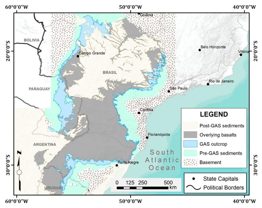
The Guarani Aquifer System (GAS) is one of the largest groundwater reservoirs in the world,
representing a transboundary system that encompasses four countries in Latin America: Argentina,
Brazil, Uruguay and Paraguay (Figure 1). Covering an area of about 1.2 million km2 , the GAS system
is regulated by an important international treaty, the Guarani Aquifer Agreement. While the average
thickness of GAS is nearly 250 m, its maximum thickness exceeds 800 m [1]. The GAS comprises a
sequence of sandy layers of Triassic-Jurassic age, deposited in continental, aeolian, fluvial and lagoon
environments, above a regional erosional surface (dated to 250/Ma) and below an extensive layer of
Cretaceous basalts (dated to 145–30/Ma) in the basins of Paraná (Brazil and Paraguay), Chaco-Paraná
(Argentina) and North (Uruguay) [2]. The Guarani Aquifer System is confined by underlying pre-GAS
deposits and overlying post-GAS deposits (Figure 1), except in outcropping areas where the aquifer
ranges mostly from confined to semi-confined.
Despite the continental scale of GAS, groundwater recharge is restricted to narrow outcrop zones,
mainly along its western and eastern borders (Figure 2). Estimates of groundwater recharge in the
outcrop zones were calculated by several authors (e.g., [3–6]). However, most groundwater recharge in
the outcrop zones is discharged into local watersheds, with only minor amounts reaching the confined
part of GAS to form deep recharge. Other studies [7,8] showed that deep recharge comprises only 10
to 15 mm/year, which represents a scant 1 to 2% of annual rainfall.
Water 2020, 12, 2323; doi:10.3390/w12092323 www.mdpi.com/journal/water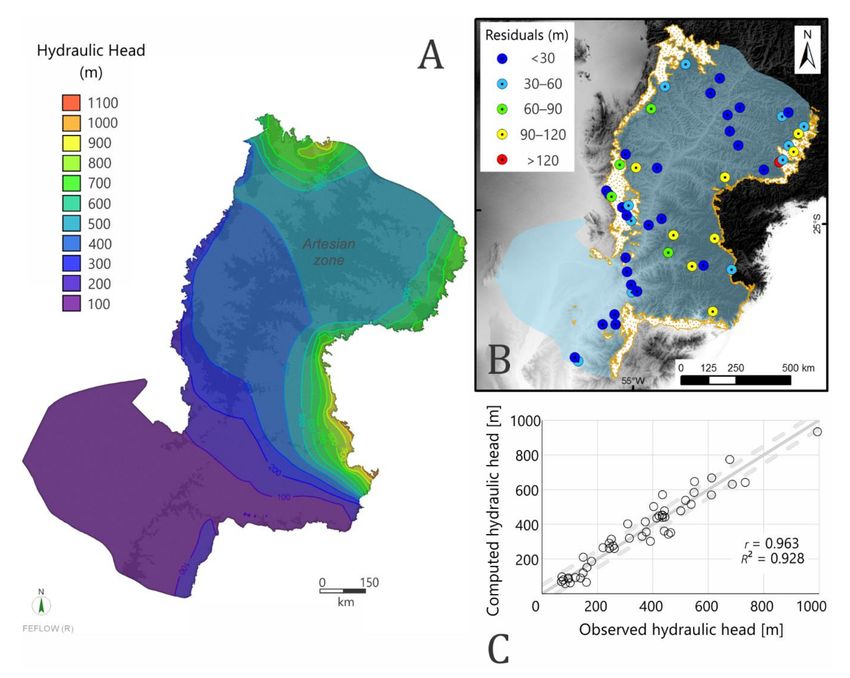
Water 2020, 12, 2323                                                                                2 of 12

      Figure 1. Simplified geologic map showing pre-GAS and post-GAS sediments, GAS outcropping areas
      and overlying basalts (modified from [9]).

     Because of its strategic importance, several studies have focused on possible actions to improve
GAS water management, sustainable use and groundwater protection [1,2,10–13]. The extensive area
underlain by GAS has a population of about 15 million, whereas 90 million inhabitants are indirectly
benefitting from GAS exploitation [10]. Thus, the need for reliable potable water and industrial
supplies (of low-cost treatment) is likely to grow significantly, especially when considering also climate
change [10]. According to [10], GAS exploitation exceeds 1.0/km3 /year, being 93.6% in Brazil (of which
about 80% occurs in São Paulo State), 2.8% in Uruguay, 2.3% in Paraguay and 1.3% in Argentina.
Approximately 80% of total water extraction is used for public water supply, 15% for industrial
processes and 5% for geothermal spas [10].
     Geological models and structural implications in terms of groundwater flow and hydrochemistry
of GAS were studied by [14–17], among others. Numerical models are crucial tools for water resources
management of continental scale aquifers. Despite the importance of GAS as a freshwater resource
and the capability of numerical models, only a few studies were previously carried out of the aquifer
system, ranging from local scale [3,4,18] to regional scale [7,17] investigations. The modeling studies
commonly calibrated the recharge fluxes by considering direct recharge in outcropping areas [3,19].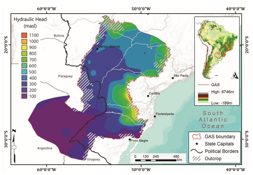
Water 2020, 12, 2323                                                                                   3 of 12

      Figure 2. Location of the study area and observed potentiometric levels (modified from [9]) of the
      Guarani Aquifer System.

      To enhance our understanding of the precise flow dynamics of the Guarani aquifer system and
obtain more reliable estimates of prevailing groundwater recharge rates, we created a three-dimensional
numerical flow model of the aquifer. The model used for this purpose was obtained using the
finite-element based FEFLOW groundwater flow simulator of [20]. In the following we first describe
our conceptual model of the GAS system, the adopted numerical model, and results of the calculations
in terms of piezometric levels, recharge estimates, and comparisons with travel time estimates within
the aquifer system using the particle tracking option of FEFLOW.

2. Conceptual Model
     Our conceptual model assumes that the GAS comprises layered sandy units and recovering
Permian aquitards (the Pre-GAS units), while being confined by basalts of varying thickness, except in
outcropping areas. While several studies suggested some hydraulic connection between GAS and
confining or underlying layers, this issue remains poorly defined. Since precise data quantifying water
exchange by inter-layer vertical flow are lacking, we assume for now that this exchange is negligible.
Henceforth, our conceptual model assumes neither recharge from nor discharge to confining basalts.
     Despite the large number of studies hypothesizing the structure and compartmentalization of GAS
in segmented blocks [15,17,21], we regarded GAS as an entirely connected block based on observed
groundwater flow continuity at the regional scale. The depositional context of GAS encompasses
aeolian, fluvial and lagoon environments. Despite local differences, the geological history of GAS
deposition points to an essentially sandy makeup, while being relatively homogeneous from a regional
point of view. We conceptualized that the diagenetic history, mainly the pore filling cement, is the
main feature controlling aquifer permeability. Figure 3 shows a schematic of our conceptual model.
Water 2020, 12, 2323                                                                                4 of 12

      Figure 3. Schematic hydrogeological cross-section showing the adopted conceptual model of the
      Guarani Aquifer System. The blue arrows show the main groundwater flow direction.

     The hydraulic conductivity (K) is a parameter known to vary with the scale of measurements [22,23],
which implies that available local-scale literature values of K may well be inappropriate due to the
large scale of the GAS. Based on an evaluation of hundreds of K measurements at different scales and
geological contexts, [22] found that as the scale increases, the mean K tends to increase until reaching
some plateau, while the variability tends to decrease with scale as the scale increases, more or less
following a potency-model. The increase in K occurs until some specific volume (the upper bound of
the relationship) is reached, after which K remains constant. An analysis of data presented by [22]
showed that K values provided by pumping tests are close to the upper bound. Consequently, we
assumed that the pumping tests served as a reliable proxy to upscaled values of K for applications at
regional scales.
     Tens of pumping tests conducted in several areas of GAS [3,24–27] showed a relatively narrow
range in K values, varying between 6.4 × 10⁻⁶ m/s and 8.1 × 10⁻⁵ m/s, with the vast majority falling
between 1.0 × 10⁻⁵ m/s and 5.0 × 10⁻⁵ m/s. Accordingly, we used these K values as constraints during
the model optimization. Furthermore, based on the assumption that GAS potentiometry is controlled
by the structural contour of the GAS basement, rather than high variability in the hydraulic conductivity,
we conceptualized that K values are relatively homogeneous, with little variation of this parameter at
the regional scale.

3. Numerical Model
      To verify the conceptual model assumptions and to calculate GAS regional flow behavior, a
three-dimensional steady-state model was constructed using the FEFLOW finite element software [20].
Two-dimensional transient models using hydraulic head fluctuations, such as done by [7], helped
to better understand the local impacts of different exchange rates, but this approach did not lead to
realistic estimates of long-term regional flow velocities. Our 3D GAS model, on the other hand, focused
on recharge rates that are consistent with estimated groundwater ages. Since our timescale is hence
millennial (up to 1 Ma), head fluctuations during the last several decades will not control our model.
Therefore, a steady-state approach is consistent and suitable for this purpose.
      The model boundary extended to the entire aquifer system, encompassing an area of 1,087,560 km2 .
The domain was divided into two layers to reflect the existence of GAS and Post-GAS units
(the latter being the younger geological units present in the basin, predominantly confining basalts).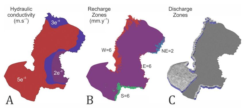
Water 2020, 12, 2323                                                                                5 of 12

The three-dimensional domain was discretized into 337,392 triangular elements and 273,864 nodes,
with irregular spacings in both the horizontal and vertical directions. The element size averaged 6 km2 ,
but with mesh refinements along the borders and larger elements in the central region.
     The domain bottom was assumed to be a no-flow boundary. In addition, seepage face boundary
conditions were introduced along the western and southeastern borders to account for the discharge
areas, thus allowing free outflow from the aquifer. Recharge rates were represented using a fluid-flux
boundary condition along the top elements over the outcropping areas. The model was calibrated
using trial-and-error methods by adjusting hydraulic conductivity values such that simulated levels
during steady-state flow agreed with the monitored hydraulic heads from 49 wells [9].
     We emphasize that underneath the major rivers (e.g., Paraná River, Figure 3) there are
approximately 1000 m of confining basalts with no reliable subsurface information to support the use
of the rivers in any calibration. The pumping from wells represents very low rates compared to overall
aquifer flow rates, albeit highly concentrated. For this reason, they are expected to locally impact the
heads, especially in the unconfined portions, but are negligible for the extremely large confined portion
of the aquifer system. In terms of ages (several hundreds of thousands of years), the impact is also
negligible. To reduce uncertainties related to non-uniqueness of the model solution, we constrained
the model parameterization using available data about groundwater age [28].

4. Results and Discussion

4.1. Piezometric Levels
     The adjusted steady-state flow model was evaluated by comparing observed and simulated
piezometric levels (Figure 4A,C). The final model simulation produced a correlation (r) of 0.9632 and a
normalized root mean square error (NRMS) of 6.04% (55.79 m) (Figure 4B,C). Model results accordingly
replicated groundwater flow patterns in terms of the hydraulic gradients and the main flow directions.
Smooth gradients were apparent near the center of the simulated aquifer, consistent with observed
potentiometry data, with the potentiometric surface being essentially flat there [29]. Higher hydraulic
gradients occurred close to the recharge areas. Regional groundwater flow was directed mainly from
the north and northeast radially towards the center and then southwards. Regional flow near the
western border was found to be somewhat fragmented by local recharge/discharge systems.

4.2. Hydraulic Conductivity
      Not enough GAS hydraulic conductivity (K) data were available to construct a regionalized
distribution map using interpolation methods such as kriging. Hence, the K zones were distributed
according to the described lithology compartments and correlated porosities [29,30]. Hydraulic
conductivities varied from about 2.5 × 10⁻⁶ m/s near the outcrops, to 5 × 10⁻⁵ m/s in the central and
southern portions (Figure 5A). Although the K zones were distributed in a relatively simplistic manner
(e.g., by using only three zones), they were geologically consistent and sufficient to reproduce the
observed regional flow patterns. The vertical K values were one order of magnitude less than the
horizontal conductivities. The fillable porosity of GAS was set uniformly at 0.2 and that of the post-GAS
at 0.0001.
      The estimated hydraulic conductivities were close to reported literature values, which showed little
variability between a minimum of 1.2 × 10⁻⁶ m/s and a maximum of 5.3 × 10⁻⁵ m/s [7]. Recent pumping
tests in São Paulo State yielded K values of about 2 to 3 × 10⁻⁵ m/s [27], similar to values reported
earlier [31]. Calibration of local scale models (100 km2 to 5000 km2 ) produced mean K values of 2.8 ×
10−5 m/s (as compiled by [7]). Our calibrated hydraulic conductivity values hence compared well with
both pumping tests and local-scale groundwater flow models. This shows that there was no need to
implement a much denser discretized K distribution as is often done for larger-scale flow models [32].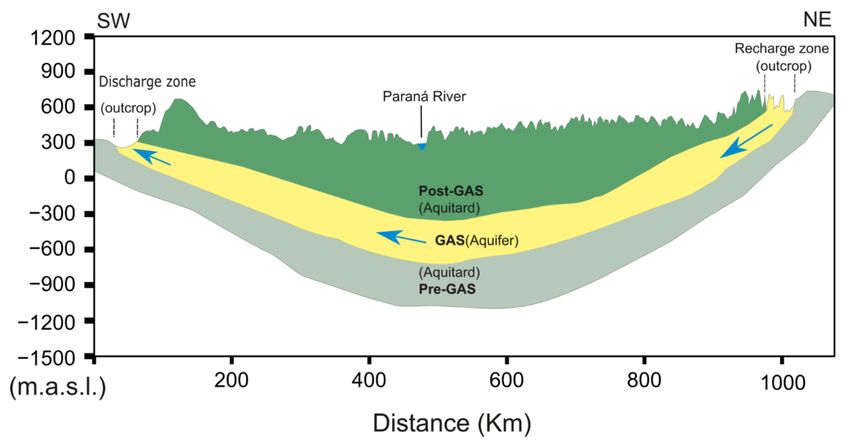
Water 2020, 12, 2323                                                                                         6 of 12

      Figure 4. (A) Calculated hydraulic head distribution, (B) map of residuals, and (C) scatter plot showing
      simulated and observed piezometric levels (in meters above mean sea level).

      Figure 5. Distributions of (A) the hydraulic conductivity, (B) recharge zones, and (C) discharge zones.

4.3. Water Budget and Recharge Estimates
     The recharge zones in the numerical model were distributed along the GAS outcrop areas
(Figure 5B), whereas the discharge zones were mostly located along the western and southeastern
borders (Figure 5C). The model was calibrated by using four recharge zones: a western zone (W)
with 6 mm/year, a northeastern zone (NE) with 2 mm/year, an eastern zone (E) with 6 mm/year, and
a southern zone (S) with a recharge of 3 mm/year. Calculated recharge for the entire domain was
approximately 0.6 km3 /year, which represents a mean average recharge rate of 4.9 mm/year.
Water 2020, 12, 2323 7 of 12
Several studies reported much higher recharge rates, generally close to 2–4% of the mean
annual precipitation rate of about 1500 mm/year [7]. For example, [33] estimated a recharge rate of
41 mm/year, whereas [7] obtained 35.2 mm/year using a more complex transient flow model (TRANSIN).
Our calculated recharge is similar to that of deep recharge into GAS (i.e., water that effectively reaches
the confined portion of the aquifer system). In a discussion of the limitations of estimating this deep
recharge, the GAS Project [9] hypothesized a volume close to 0.8 to 1.4 km3 /year, which translates to
about 6.5 to 11.5 mm/year. [34] considered deep recharge to represent less than 1% of annual rainfall
(about 1 km3 /year), but this rate could become as high as 5 km3 /year or more with increasing pumping.
Considering that some GAS portions in our model are actually discharging locally, the deep recharge
volume may be even smaller.
Much higher local recharge rates have been reported for the outcrop areas, such as by [8] who
also showed large discharge volumes into local drainage systems. Direct recharge at various GAS
sites has been estimated mostly using water balance models [3]. Hydrographs separation/analysis
techniques have been used frequently to differentiate among water sources (such as by [5] who
focused on baseflow), but also the water table fluctuation (WTF) method [35] to estimate recharge
from groundwater level fluctuations [36]. However, the WTF relies on having good estimates of the
specific yield, which is often problematic, while the recharge rates may be overestimated significantly
because of the effects of entrapped air in shallow unconfined aquifers overlaying the areas being
investigated [37]. For these reasons it is important to consider only recharge rates that effectively
contribute to the aquifer system in terms of the overall groundwater balance. Proper management
requires hence a focus on the relatively small water volumes that effectively recharge an aquifer, which
may not include water that rapidly discharges again and only influences shallow groundwater level
fluctuations and/or river outflows.
4.4. Groundwater Age Analysis
We further compared our simulations with results from groundwater dating using 81 Kr as
described by [28]. For this we performed forward streamline and travel time calculations using the
particle tracking option of the FEFLOW software. Particle seeds were positioned on the recharge
areas as shown in Figure 6A. The results revealed ages ranging mostly from 100 ky to 500 ky, with the
oldest waters reaching 1 Ma. These estimates are consistent with most of the 81 Kr dating results [28].
Some discrepancies occurred when calculating backward streamlines from the age estimates (Figure 6B),
which may reflect mixing with Pre-GAS units, as suggested by [38], or Post-GAS units (e.g., from flood
basalts), as previously discussed by [39].
The particle tracking schemes produced estimates of the advective age (also known as the true
groundwater age), which is the time needed for a water particle to move between two points purely via
advection. Particle tracking is useful since it reflects the movement of groundwater due to hydraulic
forcing as a result of hydraulic gradients, the hydraulic conductivity and porosity, and the recharge
and/or discharge rates [40]. The advective age can be used to estimate groundwater flow rates [41],
and to more directly infer recharge rates [42,43].
Our analysis of 14 wells showed three krypton ages much older than expected, two in the northern
part (728 and 834 ky) and one to the south (777 ky). These results may reflect mixing with Pre-GAS
units that contain much older water, and located relatively close to the outcropping zones. The mixing
processes in the northern portion is discussed by [38], who also included two other samples (showing
ages of 566 and 531 ky) which may have been affected by some mixing. In summary, our regional
age pattern agrees very well with most of the krypton ages. It is important to note here that we
are comparing general flow patterns within a regional context, and not trying to calibrate precisely
the ages. Thus, since krypton dating itself has considerable error margins, while only a few poorly
distributed GAS samples where available. For comparison purposes, we found that if we increased the
recharge rates ten times (to become similar to previous direct recharge estimates), values of K needed
to be increased one order of magnitude to properly calibrate the hydraulic heads. This scenario thenWater 2020, 12, 2323 8 of 12
resulted in GAS groundwater ages of only about 50 years, which is unrealistic, even when considering
mixing and preferential flow.
Figure 6. (A) Forward streamline distribution (particle tracking with travel time) by positioning
seeds on the recharge areas, and (B) backward streamlines by positioning seeds around the dated
groundwater sample locations [28].
We emphasize again that our model is regional and thus not intended for evaluating local-scale
issues in specific areas. Local problems are best addressed using local models that could provide
better support for decision-making processes. Inter-formation mixing and groundwater flow through
geological structures are certainly present and may play an important role locally [16,38,39]. However,
our results show that these exchanges are not requisite to explain overall regional flow patterns of the
GAS. Therefore, we assume that the mixing waters do not represent an important fraction of the GAS
recharge/discharge volumes.
Based on mixing simulations, [38] demonstrated very complex interactions of the Guarani Aquifer
System with both underlying and overlying units in terms of GAS receiving and delivering water.
The exact level of GAS interactions with overlying and underlying units remain largely unsolved.
Because of the complexity of this issue, we focused in our study on a relatively simplistic scenario
by assuming limited interactions of the Guarani aquifer system with other units. The capability of
our model to reproduce the hydraulic head distribution and most of the groundwater age estimates
provides confidence that the assumed scenario is feasible. Despite the disagreement about the level of
mixing with other aquifers, our simulations and those by [38] were surprising similar.
4.5. Model Discussion
Because direct measurements of discharge to the Paraná River were lacking, the potential
contribution of GAS discharge to the river is difficult to confirm directly. Contrary to the numerical
model of [7], our model assumes that the main rivers crossing the basin (e.g., the Paraná, Paraguay and
Uruguay rivers) do not represent discharge zones due to the thickness of basalts (>1000 m) beneath
them. As described by several authors [44–46], the basalt floods consist as persistent alternating thick
intervals with extremely low permeabilities (interior flows) and thin permeable intervals (top flows).
Given this situation, the significant thick basalt layers serve as very effective barriers preventing
seepage flow from GAS to the rivers.
In a practical sense, including the main rivers crossing the basin as boundary conditions may help
model calibration by modulating the simulated potentiometry. Our model, however, reveals that theWater 2020, 12, 2323 9 of 12
rivers are unnecessary to condition flow in the GAS, and that the model can be calibrated effectively
without these features, thereby reinforcing the likely absence of connectivity of GAS with the rivers.
The regional hydraulic head and distribution of groundwater reflects the natural flow conditions
stablished by long-term water flow during the last hundred millennia. Our model assumes a steady
state flow regime, thereby aiming to reproduce these conditions. Some wells in São Paulo State
experienced a noticeable, but localized, drawdown in the last four decades. We did not used this
exploitation because the effect of pumping is very restricted, without any evidence that this affected
the entire GAS (specially the confined portion). The hydraulic heads calculated with our model,
without groundwater extraction, hence will probably not adjust to heads at locations with noticeable
drawdown, thus producing a certain error. The potential error (, in %) of assuming a lack of
groundwater abstraction in our model may be estimated using the following expression:
(hcalc − hobs )
= × 100 (1)
(hmax − hmin )
where hcalc is the calculated hydraulic head [L], hobs is the observed hydraulic head [L], hmax is the
maximum hydraulic head observed in the studied aquifer [L], and hmin is the minimum hydraulic head
observed in the aquifer [L]. Assuming an extreme case, with a 50 m-drawdown induced by excessive
exploitation, the estimated error will be less than 7% as estimated using Equation (1). This indicates that
ignoring groundwater exploitation in our model will not produce a significant error when considering
the regional GAS scale.
Because the generally non-uniqueness nature of a groundwater flow model, distinct sets of
hydraulic conductivities and groundwater recharge rates often produce similar model calibrations,
leading to dissimilar water balances and high uncertainties. Our strategy to reduce uncertainties
related to the hydraulic conductivity was to carefully compile available K values of the GAS and to
force their values in the model to remain close to median of the compiled K values. Since GAS is
composed of thick sandy units deposited under aeolian to fluvial environments, the K is expected
to be relatively homogeneous at the regional scale. The ability of our model to produce reliable
potentiometry using little variability in the hydraulic conductivity field confirmed our assumption
that the hydraulic gradient and transmissivity are controlled mostly only by the structural contour of
the basement.
The use of groundwater age data as an additional calibration criterion served as an important
strategy to reduce the uncertainties related to model parameterization. Because of the direct dependence
of advective age on groundwater recharge, the degrees of freedom for producing the calibrated model
were strongly restricted. Thus, our model possessed a lower uncertainty as compared with models
calibrated exclusively with hydraulic head data.
Several studies of watersheds located in GAS outcrop zones have demonstrated that most of the
groundwater recharge discharged along the local rivers, with an exceptionally low fraction contributing
to the confined portion as deep recharge [3–5,18]. These findings closely match our results that
groundwater recharge comprises only about 1% of total precipitation. Consequently, the confirmation
of the local outcrop estimates using our 3D model covering the entire GAS has important implications
in terms of water management planning. Water extraction by well supplies in a single year comprised
17% of annual groundwater recharge, considering the recharge rates that discharge locally in the
watersheds. However, 80% (0.8 km3 ) of the extracted volume was concentrated in the populous region
of São Paulo State, in Brazil. Given this scenario, and despite our model being regional with extraction
not affecting the entire GAS, we reinforced local studies that the GAS in the São Paulo area is critically
overexploited, leading to untenable drawdown in this particular (and socially important) region.
Long-term predictions of the effects of intense groundwater exploitation in this region need to be
carried out to stablish the limit of groundwater volumes that can be extracted in a sustainable manner.Water 2020, 12, 2323 10 of 12
5. Conclusions
Because of the strategic importance of the Guarani Aquifer System and the increased demand for
water, more precise operational criteria should be defined for the sustainable use of GAS groundwater
within the context of water management. The strategies of management should be supported by
a correct diagnose of the flow dynamics and, especially, prevailing recharge rates. Our results
demonstrate that the recharge rates that effectively contribute to the regional water balance of GAS
(about 0.6 km3 /year) is much smaller than previous estimates. This is true also when comparing our
results with deep recharge approximations commonly used for water resources management. Local
discharge rates occurring in the drainage systems along outcrop zones are shown to be very high by
looking at the baseflow contribution in river hydrographs, thus only a small portion of the infiltrating
water moves deep and reaches the confined GAS.
Comparing Kr-measured groundwater ages with particle tracking and travel times showed that
higher recharge rates lead to unreasonable residence times. Moreover, when one considers smaller
specific yield (Sy ) values, which is realistic and possible, the resulted recharge rates would be even less.
This because with less fillable pore volume, less water can be stored, leading to reduced recharge rates.
Having krypton ages older as expected is evidence of some inter-formation mixing, especially with
older units. Still, this water exchange, as well as aquifer structures influencing preferential flow, were
not necessary to reproduce the GAS regional groundwater flow patterns.
For this study we used a hydrogeological model to focus on regional aspects of GAS, with a
broad view regarding aquifer homogeneity and continuity associated with age estimates. Our concern
was especially to obtain better estimates of recharge from a regional water balance perspective.
Local analyses may be needed in critical areas to test some key issues, such as inter-formation mixing,
structural controls and pumping impacts. Such studies are needed to confirm our overall findings,
as well as to beneficially use our outcomes for local scale modeling and management approaches.
Author Contributions: Conceptualization, R.D.G. and H.K.C.; methodology, R.D.G, H.K.C. and E.H.T.; validation,
R.D.G.; formal analysis, R.D.G., H.K.C. and E.H.T.; resources, H.K.C.; writing—original draft preparation,
R.D.G. and H.K.C.; writing—review and editing, R.D.G., E.H.T and H.K.C.; visualization, R.D.G.; supervision,
H.K.C.; project administration, H.K.C and R.D.G. All authors have read and agreed to the published version of
the manuscript.
Funding: This research received no external funding.
Acknowledgments: We acknowledge support for this study from the Basin Studies Laboratory (LEBAC) of the
Department of Applied Geology, associated with the Center for Environmental Studies (CEA) of UNESP and the
Foundation for Development of UNESP (FUNDUNESP), the National Counsel for Technological and Scientific
Development (CNPq), and CAPES-Brazil. We also acknowledge the scientific support and editorial review by
Rien van Genuchten.
Conflicts of Interest: The authors declare no conflict of interest. The funders had no role in the design of the
study; in the collection, analyses, or interpretation of data; in the writing of the manuscript, or in the decision to
publish the results.
References
1. Kemper, K.E.; Mestre, E.; Amore, L. Management of the Guarani Aquifer System. Water Int. 2003, 28, 185–200.
[CrossRef]
2. Sindico, F.; Hirata, R.; Manganelli, A. The Guarani Aquifer System: From a Beacon of hope to a question
mark in the governance of transboundary aquifers. J. Hydrol. Reg. Stud. 2018, 20, 49–59. [CrossRef]
3. Gómez, A.A.; Rodríguez, L.B.; Vives, L.S. The Guarani Aquifer System: Estimation of recharge along the
Uruguay–Brazil border. Hydrogeol. J. 2010, 18, 1667–1684. [CrossRef]
4. Machado, A.R.; Wendland, E.; Krause, P. Hydrologic Simulation for Water Balance Improvement in an
Outcrop Area of the Guarani Aquifer System. Environ. Process. 2016, 3, 19–38. [CrossRef]
5. Rabelo, J.L.; Wendland, E. Assessment of groundwater recharge and water fluxes of the Guarani Aquifer
System, Brazil. Hydrogeol. J. 2009, 17, 1733–1748. [CrossRef]Water 2020, 12, 2323 11 of 12
6. Rebouças, A.C. Recursos Hídricos Subterrâneos da Bacia do Paraná—Análise de Pré-Viabilidade; Universidade de
São Paulo: São Paulo, Brazil, 1976.
7. Rodríguez, L.; Vives, L.; Gomez, A. Conceptual and numerical modeling approach of the Guarani Aquifer
System. Hydrol. Earth Syst. Sci. 2013, 17, 295–314. [CrossRef]
8. Wendland, E.; Gomes, L.H.; Troeger, U. Recharge contribution to the Guarani Aquifer System estimated from
the water balance method in a representative watershed. An. Acad. Bras. Cienc. 2015, 87, 595–609. [CrossRef]
9. Organização dos Estados Americanos (OEA). Aquífero Guarani: Programa Estratégico de Ação = Acuífero Guaraní:
Programa Estatégico de Acción—Edição Bilíngüe; Organização dos Estados Americanos (OEA): Washington,
DC, USA, 2009; ISBN 978-85-98276-07-6.
10. Foster, S.; Hirata, R.; Vidla, A.; Schmidt, G.; Garduño, H. Sustainable Groundwater Groundwater Management:
Management Concepts Lessons and Tools from Practice The Guarani Aquifer Initiative—Towards Realistic
Groundwater Management in a Transboundary Context. GW Mate World Bank 2009, 1–28.
11. Villar, P.C.; Ribeiro, W.C. The Agreement on the Guarani Aquifer: A new paradigm for transboundary
groundwater management? Water Int. 2011, 36, 646–660. [CrossRef]
12. Amore, L. The Guarani Aquifer: From Knowledge to Water Management. Int. J. Water Resour. Dev. 2011, 27,
463–476. [CrossRef]
13. Rayale, K.; Little, K.; Crawford, M.; Swatuk, L. Transboundary groundwater governance and management:
The case of the Guarani Aquifer–Brazil, Argentina, Paraguay, Uruguay. In Water, Climate Change and the
Boomerang Effect; Swatuk, L.A., Wirkus, L., Eds.; Routledge: London, UK, 2018; pp. 36–49, ISBN 9781315149806.
14. Machado, J.L.F. Compartimentação Espacial e Arcabouço Hidroestratigráfico do SISTEMA Aqüífero Guarani no Rio
Grande do Sul; UNISINOS: São Leopoldo, Brazil, 2005.
15. Soares, A.P.; Soares, P.C.; Bettú, D.F.; Holz, M. Compartimentação estrutural da Bacia do Paraná: A questão
dos lineamentos e sua influência na distribuição do Sistema Aquífero Guarani. Geociências UNESP São Paulo
2007, 26, 297–311.
16. Gastmans, D.; Mira, A.; Kirchheim, R.; Vives, L.; Rodríguez, L.; Veroslavsky, G. Hypothesis of Groundwater
Flow through Geological Structures in Guarani Aquifer System (GAS) using Chemical and Isotopic Data.
Procedia Earth Planet. Sci. 2017, 17, 136–139. [CrossRef]
17. Mira, A.; Vives, L.; Rodríguez, L.; Veroslavsky, G. Modelo hidrogeológico conceptual y numérico del Sistema
Acuífero Guaraní (Argentina, Brasil, Paraguay y Uruguay). Geogaceta 2018, 64, 67–70.
18. Sapriza, G.; Gastmans, D.; De los Santos, J.; Flaquer, A.; Chang, H.K.; Guimaraens, M.; De Paula e Silva, F.
Modelo Numérico De Fluxo Do Sistema Aquífero Guarani (Sag) Em Área De Afloramentos—Artigas
(Uy)/Quarai (BR). Águas Subterrâneas 2011, 25, 29–42. [CrossRef]
19. Vives, L.; Campos, H.; Candela, L.; Guarracino, L. Modelación del acuífero Guaraní. Bol. Geol. Min. 2001,
112, 51–64.
20. Diersch, H.-J.G. FEFLOW: Finite ElementModeling of Flow, Mass and Heat Transport in Porous and Fractured
Media; Springer: Berlin/Heidelberg, Germany, 2014; ISBN 978-3-642-38738-8.
21. Gastmans, D.; Veroslavsky, G.; Kiang Chang, H.; Caetano-Chang, M.R.; Nogueira Pressinotti, M.M.
Hydrogeological conceptual model for Guarani Aquifer System: A tool for management. Boletín Geológico Min.
2012, 123, 249–265.
22. Schulze-Makuch, D.; Carlson, D.A.; Cherkauer, D.S.; Malik, P. Scale Dependency of Hydraulic Conductivity
in Heterogeneous Media. Ground Water 1999, 37, 904–919. [CrossRef]
23. Clauser, C. Permeability of crystalline rocks. Eos Trans. Am. Geophys. Union 1992, 73, 233. [CrossRef]
24. Araújo, L.M.; França, A.B.; Potter, P.E. Hydrogeology of the Mercosul aquifer system in the Paraná and
Chaco-Paraná Basins, South America, and comparison with the Navajo-Nugget aquifer system, USA.
Hydrogeol. J. 1999, 7, 317–336. [CrossRef]
25. Wahnfried, I.; Fernandes, A.; Hirata, R.; Maldaner, C.; Varnier, C.; Ferreira, L.; Iritani, M.; Pressinotti, M.
Anisotropia e confinamento hidráulico do Sistema Aquífero Guarani em Ribeirão Preto (SP, Brasil).
Geol. USP Série Científica 2018, 18, 75–88. [CrossRef]
26. Wendland, E.; Gomes, L.E.; Porto, R.M. Use of convolution and geotechnical rock properties to analyze free
flowing discharge test. An. Acad. Bras. Cienc. 2014, 86, 117–126. [CrossRef]
27. Engelbrecht, B.Z.; Teramoto, E.H.; Gonçalves, R.D.; Chang, H.K. Estimativas de condutividade hidráulica a
partir de perfilagens geofísicas no Sistema Aquífero Guarani. Holos Environ. 2020, 20, 117. [CrossRef]Water 2020, 12, 2323 12 of 12
28. Aggarwal, P.K.; Matsumoto, T.; Sturchio, N.C.; Chang, H.K.; Gastmans, D.; Araguas-Araguas, L.J.; Jiang, W.;
Lu, Z.-T.; Mueller, P.; Yokochi, R.; et al. Continental degassing of 4He by surficial discharge of deep
groundwater. Nat. Geosci. 2014, 8, 35–39. [CrossRef]
29. Gastmans, D.; Chang, H.K.; Hutcheon, I. Groundwater geochemical evolution in the northern portion of the
Guarani Aquifer System (Brazil) and its relationship to diagenetic features. Appl. Geochem. 2010, 25, 16–33.
[CrossRef]
30. França, A.B.; Araújo, L.M.; Maynard, J.B.; Potter, P.E. Secondary porosity formed by deep meteoric leaching:
Botucatu eolianite, southern South America. Am. Assoc. Pet. Geol. Bull. 2003, 87, 1073–1082. [CrossRef]
31. Sracek, O.; Hirata, R. Geochemical and stable isotopic evolution of the Guarani Aquifer System in the state
of São Paulo, Brazil. Hydrogeol. J. 2002, 10, 643–655. [CrossRef]
32. Gonçalves, R.D.; Chang, H.K. Modelo Hidrogeológico do Sistema Aquífero Urucuia na Bacia do Rio Grande
(BA). Geociências 2017, 36, 205–220. [CrossRef]
33. Chang, H.K. Proteção Ambiental e Gerenciamento Sustentável Integrado do Aquífero Guarani—Tema
3. UNESP/IGCE: São Paulo, Brazil, 2001. Available online: http://www.ana.gov.br/guarani/gestao/gest_
%20cbasico.htm (accessed on 1 August 2020).
34. Gilboa, Y.; Mero, F.; Mariano, I.B. The Botucatu aquifer of South America, model of an untapped continental
aquifer. J. Hydrol. 1976, 29, 165–179. [CrossRef]
35. Healy, R.W.; Cook, P.G. Using groundwater levels to estimate recharge. Hydrogeol. J. 2002, 10, 91–109.
[CrossRef]
36. Wendland, E.; Barreto, C.; Gomes, L.H. Water balance in the Guarani Aquifer outcrop zone based on
hydrogeologic monitoring. J. Hydrol. 2007, 342, 261–269. [CrossRef]
37. Gonçalves, R.D.; Teramoto, E.H.; Engelbrecht, B.Z.; Soto, M.A.A.; Chang, H.K.; Genuchten, M.T.
Quasi-Saturated Layer: Implications for Estimating Recharge and Groundwater Modeling. Groundwater
2019, 58, 235–247. [CrossRef] [PubMed]
38. Teramoto, E.H.; Gonçalves, R.D.; Chang, H.K. Hydrochemistry of the Guarani Aquifer modulated by mixing
with underlying and overlying units. J. Hydrol. Reg. Stud. 2020, Submitted.
39. Elliot, T.; Bonotto, D.M. Hydrogeochemical and isotopic indicators of vulnerability and sustainability in the
GAS aquifer, São Paulo State, Brazil. J. Hydrol. Reg. Stud. 2017, 14, 130–149. [CrossRef]
40. McCallum, J.L.; Cook, P.G.; Simmons, C.T. Limitations of the Use of Environmental Tracers to Infer
Groundwater Age. Groundwater 2015, 53, 56–70. [CrossRef] [PubMed]
41. Larocque, M.; Cook, P.G.; Haaken, K.; Simmons, C.T. Estimating Flow Using Tracers and Hydraulics in
Synthetic Heterogeneous Aquifers. Ground Water 2009, 47, 786–796. [CrossRef]
42. McMahon, P.B.; Plummer, L.N.; Bhlke, J.K.; Shapiro, S.D.; Hinkle, S.R. A comparison of recharge rates in
aquifers of the United States based on groundwater-age data. Hydrogeol. J. 2011, 19, 779–800. [CrossRef]
43. Solomon, D.K.; Sudicky, E.A. Tritium and Helium 3 Isotope Ratios for Direct Estimation of Spatial Variations
in Groundwater Recharge. Water Resour. Res. 1991, 27, 2309–2319. [CrossRef]
44. Navarro, J.; Teramoto, E.H.; Engelbrecht, B.Z.; Chang, H.K. Assessing hydrofacies and hydraulic properties
of basaltic aquifers derived from geophysical logging. Braz. J. Geology 2020, 50, 234–245. [CrossRef]
45. Zakharova, N.V.; Goldberg, D.S.; Sullivan, E.C.; Herron, M.M.; Grau, J.A. Petrophysical and geochemical
properties of Columbia River flood basalt: Implications for carbon sequestration. Geochem. Geophys. Geosyst.
2012, 13, 1–22. [CrossRef]
46. Rossetti, L.M.; Healy, D.; Hole, M.J.; Millett, J.M.; de Lima, E.F.; Jerram, D.A.; Rossetti, M.M.M. Evaluating
petrophysical properties of volcano-sedimentary sequences: A case study in the Paraná-Etendeka Large
Igneous Province. Mar. Pet. Geol. 2019, 102, 638–656. [CrossRef]
© 2020 by the authors. Licensee MDPI, Basel, Switzerland. This article is an open access
article distributed under the terms and conditions of the Creative Commons Attribution
(CC BY) license (http://creativecommons.org/licenses/by/4.0/).You can also read