Enhancement of Solar Energy Representation in the GCAM Model - PNNL-18829
←
→
Page content transcription
If your browser does not render page correctly, please read the page content below
PNNL-18829

Prepared for the U.S. Department of Energy
under Contract DE-AC05-76RL01830

Enhancement of Solar Energy
Representation in the GCAM Model

SJ Smith                   SD Arias
A Volke

February 2010
DISCLAIMER

This report was prepared as an account of work sponsored by an agency of the
United States Government. Neither the United States Government nor any agency
thereof, nor Battelle Memorial Institute, nor any of their employees, makes any
warranty, express or implied, or assumes any legal liability or responsibility
for the accuracy, completeness, or usefulness of any information, apparatus,
product, or process disclosed, or represents that its use would not infringe
privately owned rights. Reference herein to any specific commercial product,
process, or service by trade name, trademark, manufacturer, or otherwise does not
necessarily constitute or imply its endorsement, recommendation, or favoring by
the United States Government or any agency thereof, or Battelle Memorial
Institute. The views and opinions of authors expressed herein do not necessarily
state or reflect those of the United States Government or any agency thereof.

            PACIFIC NORTHWEST NATIONAL LABORATORY
                               operated by
                               BATTELLE
                                  for the
              UNITED STATES DEPARTMENT OF ENERGY
                   under Contract DE-AC05-76RL01830

                        Printed in the United States of America

                    Available to DOE and DOE contractors from the
                     Office of Scientific and Technical Information,
                        P.O. Box 62, Oak Ridge, TN 37831-0062;
                                     ph: (865) 576-8401
                                    fax: (865) 576-5728
                              email: reports@adonis.osti.gov

        Available to the public from the National Technical Information Service,
       U.S. Department of Commerce, 5285 Port Royal Rd., Springfield, VA 22161
                                    ph: (800) 553-6847
                                    fax: (703) 605-6900
                             email: orders@ntis.fedworld.gov
                    online ordering: http://www.ntis.gov/ordering.htm

                        This document was printed on recycled paper.
                                          (9/2003)
PNNL-18829 Enhancement of Solar Energy Representation in the GCAM Model SJ Smith SD Arias A Volke February 2010 Prepared for the U.S. Department of Energy under Contract DE-AC05-76RL01830 Joint Global Change Research Institute College Park, MD
Abstract

The representation of solar technologies in a research version of the GCAM (formerly
MiniCAM) integrated assessment model (GCAM-RE) have been enhanced to add
technologies, improve the underlying data, and improve the interaction with the rest of
the model. We find the largest potential impact is from the inclusion of thermal
Concentrating Solar Power plants, which supply a substantial portion of electric
generation in sunny regions of the world. Drawing on NREL research, domestic Solar
Hot Water technologies have also been added in the United States region where this
technology competes with conventional electric and gas technologies. PV technologies
are implemented in the CCTP scenarios, drawing on NREL cost curves for the United
States, extrapolated to other world regions using a spatial analysis of population and solar
resources.
Table of Contents
1 Introduction ................................................................................................................. 1
1.1 Research Outline................................................................................................................ 1
1.2 ObjECTS GCAM Model ................................................................................................... 1
2 CSP Electricity Generation ........................................................................................ 2
3 Domestic Solar Hot Water ......................................................................................... 5
3.1 Overview ........................................................................................................................... 5
3.2 SHW Parameters................................................................................................................ 5
3.3 Cost of SHW Service ......................................................................................................... 8
3.4 Preliminary Results............................................................................................................ 8
3.5 Fraction of Regional Demand Potentially Met by SHW ................................................... 9
3.6 Calibration/Comparison with top-down calculation ........................................................ 11
4 Rooftop Photovoltaic ................................................................................................ 11
4.1 Extension to other world regions ..................................................................................... 11
Acknowledgements ................................................................................................................... 13
5 Appendix — Mains Temperature............................................................................ 14
References ........................................................................................................................ 16
List Of Figures
Figure 1 – Auxiliary generation as a function of penetration for intermediate and peak generation
with thermal storage. .............................................................................................................. 3
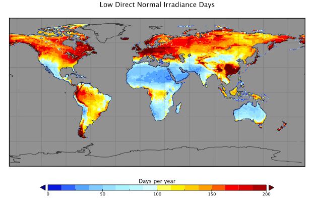
Figure 2 – Estimate of low DNI days ( < 3,000 W/m2 per day) where thermal CSP plants were
assumed to not be operational................................................................................................. 4
Figure 3 – Fraction of total U.S. electric load supplied by thermal CSP technologies under a
reference case scenario. .......................................................................................................... 4
Figure 4 – Residential hot water technology share in a reference case scenario. ............................ 9
List of Tables
Table 1 – Total distributed (rooftop) PV resource assumed for 14 GCAM model regions in EJ of
electricity generation. ........................................................................................................... 13
ii1 Introduction
1.1 Research Outline
This work is part of ongoing research to enhance the representation of renewable and
end-use energy technologies in the long-term integrated assessment model GCAM
(formerly MiniCAM). In previous work building and industrial end-use technologies
were enhanced to explicitly represent specific services such as heating, cooling, and hot
water along with specific technology options for supplying these services (Rong et al.
2007; Kyle et al. 2009, Wise et al. 2007). Previously an explicit representation of wind
technologies and resources was also implemented (Kyle et al. 2007) as well as an
enhanced representation of geothermal energy (Hannam et al. 2010).
This report describes work to date to improve the representation of solar energy
generation in the model. We have focused on three technologies: thermal Concentrating
Solar Power (CSP), domestic Solar Hot Water (SHW), and both rooftop and central
station photovoltaic technologies (PV). These are described in the following sections.
The interaction of these technologies with other renewable technologies, the rest of the
energy system, and with climate policies will be explored in the next phase of this
research. The renewable technology representations described here will be combined
with a new representation of the US electricity system that explicitly models different
load segments (Wise and Smith 2007). Using this enhanced model, focusing on the
United States, the potential role of renewable energy technologies in providing domestic
energy supply and lowering greenhouse emissions will be examined.
1.2 ObjECTS GCAM Model
The Object-oriented Energy, Climate, and Technology Systems (ObjECTS) framework
uses a flexible, object-oriented modeling structure to implement an enhanced version of
the partial-equilibrium GCAM (formerly MiniCAM) model (Kim et al. 2006). The
ObjECTS GCAM is an integrated model of the economy, energy supply and demand
technologies, agriculture, land-use, carbon-cycle, and climate. This framework is
intended to bridge the gap between “bottom-up” technology models and “top-down”
macro-economic models. By allowing a greater level of detail where needed, while still
enabling interaction between all model components, the ObjECTS framework allows a
high degree of technological detail while retaining system-level feedbacks and
interactions. By using object-oriented programming techniques (Kim et al. 2006), the
model is structured to be data-driven, which means that new model configurations can be
created by changing only input data without changing the underlying model code.
The GCAM is a partial-equilibrium model structure that is designed to examine long-
term, large-scale changes in global and regional energy systems. The GCAM has a strong
1focus on energy supply technologies and has been recently expanded to include a
comprehensive suite of end-use technologies. The GCAM (then called MiniCAM) was
one of the models used to generate the IPCC SRES scenarios (Nakicenovic and Swart
2000). This model has been used in a number of national and international assessment
and modeling activities such as the Energy Modeling Forum (EMF; Edmonds, et al. 2004,
Smith and Wigley 2006), the U.S. Climate Change Technology Program (CCTP; Clarke
et al. 2006), and the U.S. Climate Change Science Program (CCSP; Clarke et al. 2007)
and IPCC assessment reports.
The GCAM model is calibrated to 1990 and 2005 and operates in 15-year time steps to
the year 2095. It takes inputs such as labor productivity growth, population, fossil and
non-fossil fuel resources, energy technology characteristics, and productivity growth
rates and generates outputs of energy supplies and demands by fuel (such as oil and gas)
and energy carriers (such as electricity), agricultural supplies and demands, emissions of
greenhouse gases (carbon dioxide, CO2; methane, CH4; nitrous oxide,N2O), and
emissions of other radiatively important compounds (sulfur dioxide, SO2; nitrogen oxides,
NOX; carbon monoxide, CO; volatile organic compounds, VOC; organic carbon aerosols,
OC; black carbon arosols, BC). The model has its roots in Edmonds and Reilly (1985),
and has been continuously updated (Edmonds et al. 1996; Kim et al. 2006). GCAM also
incorporates MAGICC, a model of the carbon cycle, atmospheric processes, and global
climate change (Raper et al. 1996; Wigley and Raper 1992).
The detailed representations described here have been implemented and tested in a
version of the GCAM that will be identified in this report as GCAM-RE (GCAM-
Renewables).
2 CSP Electricity Generation
Thermal Concentrating Solar Power (CSP) plants concentrate direct solar radiation to
produce heat and generate electricity using a turbine or thermal engine. One advantage of
CSP technologies is that generation at times when solar radiation is not available can be
provided by use of an auxiliary heating system, which is a low capital cost addition to the
plant. All current plants are built as hybrid plants enabling them to provide firm power.
CSP technology used in this way, therefore, sidesteps the intermittency issue.
CSP technology in the GCAM-RE model is implemented as described in the PNNL
report by Zhang and Smith (2008) and in a submitted journal paper (Zhang et al 2009).
Details of the implementation can be found in these documents. Separate technologies are
implemented for intermediate and peak generation without thermal storage, intermediate
and peak generation with several hours of thermal storage, and baseload generation with
large amounts of thermal storage.
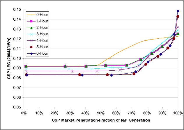
As described in the above references, a parameterization was developed (Figure 1) that
determines the use of auxiliary generation as a function of penetration. Similarly, the
2amount of solar energy lost due to exceeding demand as a function of penetration is also
parameterized.
Figure 1 – Auxiliary generation as a function of penetration for intermediate and peak
generation with thermal storage.
We find that a critical parameter characterizing the performance of CSP technologies is
the number of days of low direct normal irradiance when this technology cannot operate.
This data is not generally available, although it can be approximated using the National
Solar Radiation Data Base (NSRDB). We developed a correlation between the NSRDB
and globally gridded parameters from NASA to estimate the number of low direct normal
irradiance (DNI) days globally (Figure 2). Average irradiance on sunny days is much
more similar in different world regions than total direct normal irradiance, which
averages over low DNI days, making the estimate of low DNI days an important priority
for future research.
In prime areas with relatively few low DNI days, CSP technologies need to consume
little backup fuel (assumed to be either natural gas or biomass). In areas with a larger
number of lowDNI days, CSP technologies can still have a role, acting in essence as fuel
extenders by combining solar energy with either natural gas or biomass.
A key feature of the solar resource is that high quality solar resource is generally spatially
concentrated within most regions. Therefore, assumptions are necessary for the extent to
which electricity generated in sunny regions can be transmitted to other regions. In a
reference case set of assumptions CSP power can provide the largest share of
intermediate and peak generation and a significant fraction of baseload generation in
those regions with good quality CSP resources. A more substantial expansion of CSP will
require large-scale transmission capacity to transmit power to regions more distant from
the highest quality solar resources.
32
Figure 2 – Estimate of low DNI days ( < 3,000 W/m per day) where thermal CSP plants
were assumed to not be operational.
Figure 3 shows the fraction of US electric load under a reference case scenario (Zhang et
al. 2009). We find that CSP is highly competitive as technology serving intermediate and
peak loads. Systems without thermal storage are competitive but systems with thermal
storage are more competitive if these are developed and deployed as assumed here. In the
US south-west and west where the highest quality solar resources are located we find
CSP technologies are capable of providing a large fraction of intermediate and peak load.
Fraction of US Electric Load
4%
Interm&Peak_no Storage
Interm&Peak_Therm Storage
3% Baseload
2%
1%
0%
2000 2020 2040 2060 2080 2100
Year
Figure 3 – Fraction of total U.S. electric load supplied by thermal
CSP technologies under a reference case scenario.
4Baseload CSP plants with around 12 hours of thermal storage become more competitive
later in the century and supply an increasing share of US electricity as costs are assumed
to decline over time.
3 Domestic Solar Hot Water
3.1 Overview
Solar domestic hot water (SDHW) systems in the United States region are implemented
in GCAM-RE as additional technologies that can supply hot water service. These
technologies are implemented in a similar manner to the other building end-use
technologies, that is, with an efficiency and an amortized capital and maintenance cost.
Solar hot water technologies will also be subject to a capacity limit which represents
buildings that cannot be serviced by this technology due to shading or building type, such
as high-rise buildings. For consistency with other solar work for GCAM these
calculations are conducted globally using GIS tools and global data sets so that these
results can potentially be applied to all regions in the model and to US sub-regions if
desired.
3.2 SHW Parameters
To implement SHW in the GCAM-RE model we will take advantage of the finding of
Christensen and Barker (1999) that solar system efficiency, defined as energy savings
divided by incident solar energy, is roughly constant across a wide range of climatic
zones. As a formula, this becomes:
sav
E conv E SHW
aux _ sav
1) CSHW , where
E solar
sav
E conv = Amount of energy consumed by a conventional hot water system not
including losses. (see below)
aux _ sav
E SHW = Amount of auxiliary energy consumed by the solar hot water system not
including tank losses. (see below)
E solar = Amount of solar energy incident on the solar hot water collector
CSHW = A constant that characterizes a particular solar hot water system (referred to
by Christensen and Barker (1999) as the system efficiency)
The formulation in Equation (1) is, formally, slightly different than the definition used by
Christensen and Barker (1999) in that our formulation would formally include other
changes in the overall system efficiency due to the operation of a solar hot water system
as compared to a conventional hot water system. For properly sized systems, these
5differences should generally be negligible.1 Given the aggregate nature of our application,
this simplification does not introduce significant error compared to other uncertainties.
The constant CSHW has a small dependence on ambient temperature; however for
purposes of this project these will be neglected. There is a significant dependence on
water draw amount, whereby CSHW decreases significantly as the draw amount decreases
(from 0.43 to 0.33 as the draw was halved from 300 liters/day to 150 liters/day). Given
the national level of this implementation it is difficult to determine the appropriate
average value for water draw. However, given that our top-down calibration (see below)
indicates an average daily water draw on the low end of the consumption range, we use
the intermediate assumption of 225 liters/day draw and a base value for CSHW = 0.39. A
newer algorithm for mains temperature and adjustment for pipe losses reduces this value
to CSHW = 0.36. (J. Burch, pers com), which is the value used in this work.
Two of the terms in Equation (1) can be estimated for any given point on the globe given
sav
data developed as part of this project: E conv and E solar . The incident solar energy is
simply the average annual solar irradiance times the solar collector area. Solar irradiance
is taken from the NASA SEE estimate, where we used annual average values for the
radiation on equator-pointed 48 Degree tilted surfaces.
sav
The energy needed for conventional water heating ( E conv ), not including losses, is
approximately equal to:
2) sav
E conv c p V Thw Tmains /recov , or
the annual hot water draw (V) times the specific heat of water and the annual average
temperature difference between mains and the hot water set point over the conventional
water heater energy recovery efficiency. A set point of 55°C (Christensen and Barker
1999) is assumed. The estimate of mains temperature used here is described in the
appendix. The energy recovery efficiency is the instantaneous efficiency of the auxiliary
heating system not including conductive and diffusive losses, and is approximately 1 for
electric systems and 0.82 for gas-fired systems. The energy recovery efficiency is used in
the calculation of energy savings (Equation 1) instead of the net system efficiency (also
called the energy factor) because other system losses are, to first order, common to both
solar and conventional systems.1
Solving for auxiliary energy demand,
3) aux _ sav
E SHW E conv
sav
CSHW E solar .
A population-weighted average estimate for the amount auxiliary heat demand can be
calculated for each region given the two quantities estimated above. For consistency with
the source calculation for the system efficiency constant we assume a collector area of
1
Thanks to Jay Burch (pers communication) for pointing out this distinction.
63.72 m2 (Christensen and Barker 1999) for this calculation. Following Christensen and
aux _ sav
Barker (1999) we place a limit of E SHW 0.2E conv
sav
for each grid cell
In its simplest form, GCAM operates with two inputs for each technology, an amortized
capital plus non-fuel O&M cost and an I-O coefficient that represents the amount of
energy input needed for a unit of service output (this is an inverse efficiency). Because
the “efficiency” for SHW can be > 1 for sunny regions, for clarity, we will work with I-O
coefficients. Because energy demand is inversely proportional to efficiency, the I-O
coefficient for the SHW technology will be related to the efficiency of a conventional
technology as:
aux _ sav
E SHW
4) C SHW
I O sav
conv ,
E conv
or in terms of efficiency,
sav
E conv
5) SHW
conv aux _ sav
,
E SHW
where the energy quantities are regional average values as calculated above and conv is
the system efficiency (energy factor) for the conventional system. As above, we have
assumed that losses from the storage tank are similar for both systems.2 SHW heaters
could potentially use either electric or gas backup systems, and both are included as
options.
The total cost of both conventional and SHW technologies will have a central value and a
distribution that depends largely on geographic location, but also on fuel cost variations.
This is the situation described by Clark and Edmonds (1993) where the logit choice
formulation used in the GCAM model is applicable. While the logit choice mechanism is
strictly applicable if the shapes of the distributions are identical, given the many
uncertainties, any error introduced by this inconsistency is acceptable. In this case, the
cost distribution for SHW systems is best fit by a logit exponent of -3, which is a much
wider cost distribution than that for conventional systems.
For the USA, where we can embed the SHW technology into the detailed buildings
model, the fraction of regional demand that can be supplied by SHW (see below) can be
implemented into the model as a capacity limit.
2
Equation 4 formally would use the actual conventional and auxiliary energy consumption, however,
both of these are proportional to the _sav quantities with a conversion factor of recov /conv , which
cancels.
7For other regions (and the aggregate USA buildings implementation) the solar hot water
supply sector would have to compete as another technology option in the aggregate
buildings representation. This could be done similarly to the USA detailed version except
the capacity limit would also need to incorporate the fraction of the total building demand
for hot water services. This may be investigated in the future. An additional issue is the
amount of hot water demand per person in other world regions. In many world regions
per-capita hot water demand is much lower than in the United States. Values for Japan
and/or Europe could be used for other world regions.
3.3 Cost of SHW Service
The cost of SHW service can be broken into two parts: the capital and (non-fuel) O&M
costs of the SHW system, and the cost of purchasing backup energy. The total cost of
conventional and solar hot water heating, respectively, would therefore be:
6) cost of SHW: c SHW c SHW
fuel , and
cost of Conv HW: c conv c conv
fuel ,
where cconv and cshw are the amortized capital and maintenance costs for conventional and
solar hot water systems respectively, and the second terms are annual fuel costs.
The amortized capital and O&M costs for the SHW systems will be determined using the
same financing assumptions as used for conventional hot water systems. One significant
difference, however, is lifetime. Many conventional hot water systems have relatively
short lifetimes, and low capital cost. SHW systems generally have longer lifetimes of
around 20 years.
3.4 Preliminary Results
Figure 4 shows a preliminary calculation of the penetration of SHW systems in the
United States under a reference case with no climate policy. Capital costs for SHW were
assumed to be $6,000 in 2005 as found in a recent review of costs in California (KEMA
2009), declining by 2% per year. The cost used here is similar to the average active
system cost of $4,960, found in a market review conducted by the authors, assuming
installation costs are 23% of total cost (KEMA, Inc.). A review conducted in New York
state, however, found much higher costs of $9,000-$11,000 for flat panel systems
(Perlman & McNamara 2008), in part due to much larger installation costs averaging
50% of total cost. While these costs are from different studies that may not have similar
methodologies, it appears that costs for a colder climate such as New York may be
substantially higher than costs in sunnier regions. In the implementation proposed here,
the installed cost should be an average cost in areas where solar systems could be used. If
this cost differential proves to be accurate, then further consideration of the appropriate
value for the assumed average installed cost would be warranted.
8In this preliminary implementation (Figure 4), SHW systems begin to provide a
significant fraction of hot water service by mid-century once system costs were assumed
to have decrease. The capital cost of SHW systems was assumed to decrease by 2% pear
year between 2005 and 2035 and 1% per year thereafter, resulting in capital costs
approximately twice that of conventional systems by the end of the century.
Electric heat pump technologies increase market share at the expense of conventional
technologies due to their higher efficiencies and increases in the cost of natural gas. Solar
technologies can be even more efficient than heat pumps in terms of energy savings, but
are more expensive so are competitive only in particularly sunny areas where auxiliary
fuel use is low. We also find that the manner in which the technology competition within
the model is structured makes a significant difference in model results. These details will
be examined further in the next phases of this research.
Figure 4 – Residential hot water technology share in a reference case scenario.
3.5 Fraction of Regional Demand Potentially Met by SHW
The final necessary data element needed is an estimate of the fraction of the total hot
water demand that can potentially be met by SHW. This sets an upper limit on the
amount of SHW penetration. All domestic hot water demand in a region that is not
considered excluded by the above considerations can potentially be supplied by SHW
systems. No detailed studies on rooftop availability for SHW systems have been
conducted, and what analysis has been done is focused on PV systems. Further, the little
information that does exist is on the basis of fraction of roof area available for PV, as
opposed to fraction of households that have sufficient suitable roof area available for a
SHW system, which occupy much less space than most rooftop PV systems and have
9looser constraints in regard to shading. We consider the assumptions made here
reasonable, but quite uncertain.
The ability to install a SHW system will depend on housing type, shading, and roof
orientation. For housing type, we use population density as a surrogate variable as this is
globally available at relatively high resolution. In order to map from housing type to
population density we drew on the compilation of Campoli and MacLean (2007) to
determine how housing density relates to rooftop availability for SHW systems. From
this compilation we estimate that limits on rooftop availability begin at about 3 housing
units per acre and that, by 50 housing units per acre, few opportunities exist for rooftop
installations. At these higher densities multi-story units become more common and the
amount of available rooftop space is relatively small compared to the number of units in a
building. To convert from housing density to population density we assume the number
of persons per household to decline from 2.8 to 2.0 as the housing unit density goes from
3 to 50 units per acre (Bennefield and Bonnette 2003). To convert from a neighborhood
scale to landscape scale we assume 20% of the land is not occupied by residential
buildings.
Rounding the result, we, therefore, assume that no residential rooftop area is available for
2
SHW systems when population density is higher than 13,500 persons per km , that 100%
of the residential rooftops are potentially available for population densities below 1,500
2
persons per km , with a linear interpolation in between these limits. The fraction of US
population excluded due to high densities is 7%. The only regions with a substantial
fraction of their population excluded are Japan and Korea, with 23% and 40% excluded,
respectively.
The shading factor is calculated from global gridded data of potential forest cover
(Ramankutty and Foley 1998) and roof shading assumptions. Drawing from Chaudhari et
al. (2004), we assume that 65% of the residential buildings in areas that have natural
forest cover have sufficient un-shaded rooftop space for SHW systems while we assume
the shading by trees in other areas (with no native tree cover) is not extensive enough to
prevent SHW system installation. Shading by other causes or other issues (roof shape,
nearby buildings, etc.) is assumed to reduce potential installations by 10%.
Residential roof orientation is assumed accessible to solar water heating in 83% of homes
(Chaudhari et. al, 2004). Pitched roofs make up 92% of residential roofs while flat roofs
make up 8%. Flat roofs are oriented in the correct direction 100% of the time. Pitched
roofs are 75% gable ended with two pitched sides, and 25% hip roofs with four sides. Of
the gable roofs, 75% are assumed to have one half of the roof facing the correct solar
orientation, while hip roofs have four sides with one facing the optimum solar orientation.
The combined roof type, population density, and shading factors result in an assumption
that SHW systems can potentially be used by 40-70% of the US population, depending
on region. The average value for the US is 60%. This is slightly higher than the
assumptions in Denholm (2007), who derived a United States average value of 50%.
103.6 Calibration/Comparison with top-down calculation
For consistency, and to ensure an accurate comparison within the model framework, the
results of the bottom-up calculations should be compared with the top-down calculations
used to calibrate the model. Residential hot water consumption in the GCAM USA
buildings model was calibrated using energy consumption data from RECS and stock
average water heater efficiency (system efficiency, a.k.a. energy factor) derived from
stock data used in the NEMS modeling system. The average installed stock system
efficiency used for calibration was 54% for gas and 86% for electric hot water heaters.
The top-down calculation resulted in a value for hot water service 40% smaller than the
value calculated using an average household water draw of 243 L/day (SRCC/GAMA =
64 gallons/day), a hot water set temperature of 57.1 °C, a US population-weighted mains
temperature of 13.4 °C, and 103,246,000 households.
Any number of biases and data uncertainties can contribute to this difference. It is
possible that the RECS data underestimates hot water consumption. For calibration
purposes, we propose to split the difference and assume that the actual hot water draw is
lower than the SRCC value, but larger than that implied by the RECS data. This is
consistent with some recent studies that indicate hot water usage in the 50 gal/day range
(J. Burch pers com), comparable to the adjusted value we assume here.
If the stock average efficiency is underestimated this would contribute to this difference.
However, 30% or more of US households report water heaters at least 10 years old
(RECS 2005), so there is a limit to how high the average stock efficiency might be.
4 Rooftop Photovoltaic
Photovoltaic technologies are implemented in GCAM as described in Clarke et al. (2008).
PV supply curves developed by NREL (Denholm and Margolis 2008) used data on solar
irradiance and the distribution of buildings, and assumed a mix of orientations to produce
a supply curve for distributed PV generation. This curve is used to represent rooftop PV
in the United States and is assumed to shift over time as PV technology costs decline.
Effectively, a net metering assumption was assumed. Distributed PV was assumed to
compete with grid-produced electricity at the meter, so that the price of distributed PV is
compared to the delivered cost from the electric grid.
4.1 Extension to other world regions
For CCTP and other global analysis, a representation of distributed PV technologies is
needed for other world regions. To produce a global estimate for distributed PV supply
we used a simple procedure whereby the US supply curve was scaled to account for
population distribution, solar resource, and family size. Ideally, regional estimates for
rooftop area should be used, but these are not available.
11To account for regional differences in solar irradiance, the population-weighted solar
irradiance for each model region was estimated using NASA Surface meteorology and
Solar Energy data. The entire US resource curve was scaled by the estimated value of
total irradiance relative for each region relative to the US value calculated in the same
manner. This takes into account regional differences in solar radiation levels.
The total solar resource was then adjusted to account for the total population in each
region. We assume that the total distributed solar “resource” to be proportional to the
population in each region with corrections for population density and household size. The
solar resource curve calculated by Denholm and Margolis (2008) assumed 1) no PV
installations in multi-story buildings due to a combination of limited rooftop area and
other uses for rooftop space and 2) a smaller solar installation on attached homes (e.g.
townhomes, etc.). In our extrapolation to other regions we used population density as a
surrogate for explicit information on building types, assuming lower overall PV
installations as population density increases. To correct for population density we
determined the “effective population” of each region for purposes of scaling by summing
2
population within each region with a population density cap of 1000 persons/km , and
2
excluding areas with population densities greater than 2000 persons/km . Thus, we
assume that PV installations will be proportional to population density until a population
2
density of 1000 persons/km , at which point no further increase is assumed to occur.
2
Areas with population densities greater than 2000 persons/km are assumed to be
primarily high-rise buildings with limited rooftop area available for PV installations. The
calculation was conducted at a 5 minute resolution using the Gridded Population of the
World version 3 (CIESIN 2005).
The final adjustment was for household size. Regional with a higher number of persons
per household were assumed to have more persons per dwelling and, therefore, would
have a lower per-capita availability of rooftop space for PV installations. The PV
resource curve was, therefore, multiplied by the ratio of household size relative to the US
for each region. Formally, there is nothing in this analysis that limits distributed PV
installations to rooftops. It is conceivable that much of the distributed PV installed could
be located nearby, but not on top, of dwellings or other structures. In residential areas,
however, there may be significant limits to the amount of space that residents may wish
to devote to PV installations. Average regional household sizes were determined
The resulting maximum distributed solar PV resource for each region is given below.
The adjustments shown are cumulative from left to right, with the right-hand column
being the final, adjusted total resource. Adjusting for average irradiance increases the
available resource in sunny regions (e.g., Australia/NZ, Middle East, Africa) and
decreases the resource in cloudy regions (FSU, Eastern Europe). Adjusting for the
combination of population and population density dramatically changes the resource.
Very large resources result in sunny regions with large populations such as China, Africa,
and India. Scaling by household size reduces the total distributed PV resource for these
regions.
12To roughly account for increases in housing area over time, the PV resource is assumed
to grow slightly as a function of GDP. While there is projected to be significant
population growth in many of these regions, much of this growth, particularly in
developing countries, will likely occur in dense urban areas, which would not necessarily
result in large increases in distributed PV relative to the current estimated potential. A
more rigorous accounting of rooftop PV availability would require a more detailed
description of population changes over time, including rural, suburban, and urban
population levels along with changes in household size and, ideally, floor space and
building characteristics (multi-story, attached, high-rise, etc.).
Total Distributed PV resource
Scaled by average Scaled using Scaled by household
irradiance population density size
USA 2.7 2.7 2.7
Canada 2.2 0.2 0.2
Western Europe 2.3 3.6 3.0
Japan 2.5 0.7 0.6
Australia_NZ 3.2 0.3 0.2
Former Soviet Union 2.2 2.1 1.7
China 2.7 14.3 9.2
Middle East 3.6 2.5 1.1
Africa 3.6 11.2 5.2
Latin America 3.3 5.8 3.4
Southeast Asia 3.3 9.1 4.6
Eastern Europe 2.2 1.1 0.9
Korea 2.7 0.5 0.3
India 3.3 12.8 6.0
Table 1 – Total distributed (rooftop) PV resource assumed for 14 GCAM model regions
in EJ of electricity generation.
Acknowledgements
The authors would like to thank Jay Burch for many useful discussions and insights on
solar hot water systems. This work was funded by the U.S. Department of Energy’s
Office of Energy Efficiency and Renewable Energy with additional support from the
Global Energy Technology Strategy Program (GTSP) and the US Climate Change
Technology Program (CCTP).
135 Appendix — Mains Temperature
In order to estimate the energy needed for hot water heating, an estimate of the average
temperature of water mains, or more precisely – the difference between ambient and
mains temperature, is needed. In regions with abundant data, algorithms can be used to fit
data to appropriate functional forms for detailed analysis of specific locations (Burch and
Christensen 2007). Here we use a global assimilation data set to estimate mains
temperature in all world regions as broad averages over one degree grid cells.
Ground temperature 2 meters deep is used as water mains temperature ( Tm ) (RETScreen,
2009). In this approximation the mains temperature depends on surface temperature with
a sinusoidal lag term that depends on depth and soil thermal diffusivity. A minimum
mains temperature of is 1º C is assumed.
Mains temperature at every grid point is estimated drawing from Hillel (1982) as:
2 (t t0 ) z
T m Ts A0e z / d sin
s d 2
Where,
Tm = mains temperature
t = day of year
d = dampening depth
t 0 15; time lag from arbitrary starting date of January 1 to day of
minimum temperature
z = depth (m);
A0 = annual temperature amplitude
t s = average annual earth skin temperature.
Ts is the average annual earth skin temperature from NASA Surface meteorology and
Solar Energy Global Data, t is the day of year, t0 is the time lag from an arbitrary start
date which is January first until the day with the minimum temperature of the year. The
annual temperature amplitude is also from NASA Surface meteorology and Solar Energy
Global Data.
We evaluate the above function for the median day of each season using the following
assumptions:
( t0 = 15) January 15 is used as the coldest day of the year (Burch, 2007).
t is calculated using the median day of each season.
o Spring= day 90 (April 15)
o Summer= day 181 (July 15)
o Fall= day 273 (October 15)
14o Winter= day 350 (January 15)
The damping depth d (m) is calculated as (Hillel, 1982)
1/ 2
2D
d h
,
2
where , and Dh is the thermal diffusivity taken as the average of four soil types
365
listed below. Permafrost and rock soils are not included. The average soil thermal
diffusivity found is 0.04235.
Soil Thermal Diffusivity ( Dh ) in m 2 / s (RetScreen, 2009)
Heavy soil- damp
(clay, compacted
sand, loam) 6.45x 10⁷
Heavy soil- dry
(clay, compacted
sand, loam) 5.16x 10⁷
Light soil- damp
(loose sand, silt) 5.16x 10⁷
Light soil- dry
(loose sand, silt) 2.84x 10⁷
15References
Bennefield R., Bonnette R. (2003) “Structural and Occupancy Characteristics of Housing: 2000.” US
Census Bureau. Washington, DC.
Burch, J., Christensen, C. (2007) “Towards Development of an Algorithm for Mains Water Temperature.”
Proceedings of the 2007 ASES Annual Conference, Cleveland, OH.
Campoli J., MacLean A.S. (2007) “Visualizing Density”. Lincoln Institute of Land Policy.
Center for International Earth Science Information Network (CIESIN), Columbia University; and Centro
Internacional de Agricultura Tropical (CIAT) (2005) Gridded Population of the World Version 3
(GPWv3): Population Density Grids. Palisades, NY: Socioeconomic Data and Applications Center
(SEDAC), Columbia University.
Chaudhari M., Frantzis L., Hoff T.E. (2004) “PV Grid Connected Market Potential in 2010 under a Cost
Breakthrough Scenario.” prepared by Navigant Consulting for The Energy Foundation.
Christensen C. and Barker G. (2003) “Annual Efficiencies for Solar Water Heating”. Proc. ASES 1999,
ASES, Boulder, CO.
Clarke J.F. and Edmonds J.A. (1993) “Modeling Energy Technologies in a Competitive Market”. Energy
Economics, 123-129.
Clarke, L., M. Wise, J. Edmonds, M. Placet, P. Kyle, K. Calvin, S. Kim, and S. Smith (2008). CO2
Emissions Mitigation and Technological Advance: An Updated Analysis of Advanced Technology
Scenarios. Pacific Northwest National Laboratory, PNNL-18075.
Clarke L. E., Wise M. A., Lurz J. P., Placet M., Smith S. J., Izaurralde R. C., Thomson A. M., Kim S. H.
(2006) “Technology and Climate Change Mitigation: A Scenario Analysis.” PNNL-16078.
Clarke L., Edmonds J., Jacoby J., Pitcher H., Reilly J., Richels R. (2007) “Scenarios of Greenhouse Gas
Emissions and Atmospheric Concentrations”. Report by the U.S. Climate Change Science Program and
approved by the Climate Change Science Program Product Development Advisory Committee (United
States Global Change Research Program, Washington, D.C.).
Denholm P. (2007) “The Technical Potential of Solar Water Heating to Reduce Fossil Fuel Use and
Greenhouse Gas Emissions in the United States”. (NREL/TP-640-41157).
Denholm P. and Margolis R. (2004) “Very Large-Scale Deployment of Grid-Connected Solar
Photovoltaics in the United States: Challenges and Opportunities” Conference Paper, NREL/CP-620-
39683
Edmonds J. A., Clarke J. F., Dooley J. J., Kim S. H., Smith S. J. (2004) “Modeling Greenhouse Gas
Energy Technology Responses to Climate Change.” Energy 29(9-10): 1529–1536.
Edmonds J. and Reilly J. (1985) “Global Energy: Assessing the Future”. Oxford, United Kingdom: Oxford
University Press.
Edmonds J. A., Wise M., Pitcher H., Richels R., Wigley T., MacCracken C. (1996) “An integrated
assessment of climate change and the accelerated introduction of advanced energy technologies: An
application of MiniCAM 1.0.” Mitigation and Adaptation Strategies for Global Change 1(4): 311–339.
GAMA. (1994) “April 1994 GAMA Consumers’ Directory of Certified Efficiency Ratings for Residential
Heating and Water Heating Equipment.”
Hannam, P., G.P. Kyle, S. Smith (2010) Impacts of Advanced Geothermal Technology on Global Energy
Production: Using a New Characterization in MiniCAM (PNNL-19231).
Hillel, D. (1982) “Introduction to Soil Physics.” Academic Press. San Diego, CA.
KEMA Inc. (2009) “California Energy Commission Staff Workshop Building and Community Scale
Renewable Technology Costs”. California Energy Commission.
Kim S., Edmonds J., Lurz J., Smith S.J., Wise M. (2006) “Hybrid Modeling of Energy-Environment
Policies: Reconciling Bottom-up and Top-down.” The Energy Journal, special issue #2.
16P. Kyle, Clarke, L., F. Rong, and S. J. Smith (2009) Climate Change and the Long-Term Evolution of the
U.S. Buildings Sector, The Energy Journal 31(3), 131-158.
Kyle P, Smith S.J., Wise M.A., Lurz JP, Barrie D. (2007) “Long-Term Modeling of Wind Energy in the
United States” PNNL-16316.
McNamara A., Perlman J. (2009) "Solar Domestic Hot Water Technologies Assessment." NYSERDA
Report 08-09.
Nakicenovic, N., and R. Swart, eds. (2000) “Special Report on Emissions Scenarios”. Cambridge, U.K.:
Cambridge University Press.
NASA. (2009) “Surface meteorology and Solar Energy A renewable energy resource web site (release
6.0).” < http://earth-www.larc.nasa.gov/cgi-bin/cgiwrap/solar/sse.cgi?+s01+s07#s07>.
National Solar Radiation Data Base. ()“Data Sets”. < http://rredc.nrel.gov/solar/old_data/nsrdb/>
Raper, S. C. B., Wigley T. M. L., Warrick R. A. (1996) “Global sea level rise: Past and future.” In Sea-
Level Rise and Coastal Subsidence: Causes, Consequences and Strategies. Milliman, J. D., and B. U.
Haq, eds. Kluwer Academic Publishers. 11–45.
Ramankutty N. and Foley J.A. (1999) “Estimating Estimating Historical Changes in Global Land Cover:
Croplands from 1700 to 1992.” Global Biogeochem. Cycles, 13(4), 997–1027.
Residential Energy Consumption Survey (RECS). (2005) “2005 Status Report”. Energy Information
Administration
RETScreen Version 4.0. 25 May, 2009.
Rong, F., L. Clarke, and S. J. Smith (2007) Climate Change and the Long-Term Evolution of the U.S.
Buildings Sector PNNL-SA-16869.
Smith S. J., and Wigley T. M. L. (2006) “Multi-Gas Forcing Stabilization with the MiniCAM.” The Energy
Journal, Special Issue #3.
Solar Rating & Certification Corporation (SRCC). (2008) “Directory of Solar Water Heating Systems
Meeting Minimum Operating and Performance Requirements OC 300.”
Wigley, T. M. L., and Raper S. C. B. (1992) “Implications for Climate and Sea-Level of Revised IPCC
Emissions Scenarios.” Nature 357(6376): 293–300.
Wise M.A., Smith S.J. (2007) “Integrating Renewable Electricity, Electricity Demand, and Electricity
Storage: A New Approach for Modeling the Electricity Sector in ObjECTS.” PNNL-16500.
Wise M.A., Sinha P, Smith S.J., Lurz JP. (2007) “Long-Term US Industrial Energy Use and CO2
Emissions”. PNNL-17149.
Zhang Y, Smith S.J. (2008) “An Evolutionary Path for Concentrating Thermal Solar Power Technologies”.
Solar 2008 PNNL-SA-57474.
Zhang, Y., SJ Smith, GP Kyle, and PW Stackhouse Jr. (2009) Modeling the Potential for Thermal
Concentrating Solar Power Technoogies Submitted to the Energy Journal
17You can also read