Three-Dimensional Electron Microscopy Simulation with the CASINO Monte Carlo Software
←
→
Page content transcription
If your browser does not render page correctly, please read the page content below
SCANNING VOL. 33, 135–146 (2011)
& Wiley Periodicals, Inc.

Three-Dimensional Electron Microscopy Simulation
with the CASINO Monte Carlo Software
HENDRIX DEMERS1, NICOLAS POIRIER-DEMERS1, ALEXANDRE RÉAL COUTURE1, DANY JOLY1, MARC GUILMAIN1,
NIELS DE JONGE2, AND DOMINIQUE DROUIN1
1
 Electrical and Computer Engineering Department, Universite de Sherbrooke, Sherbrooke, Quebec, Canada
2
 Department of Molecular Physiology and Biophysics, Vanderbilt University School of Medicine, Nashville,
Tennessee

Summary: Monte Carlo softwares are widely used to                   Introduction
understand the capabilities of electron microscopes.
To study more realistic applications with complex                       Electron microscopes are useful instruments that
samples, 3D Monte Carlo softwares are needed. In                    are used to observe and characterize various types of
this article, the development of the 3D version of                  samples: observation of complex integrated circuits,
CASINO is presented. The software feature a gra-                    small nanoparticles in biological samples or nanopre-
phical user interface, an efficient (in relation to                  cipitates, and dislocations by cathodoluminescence
simulation time and memory use) 3D simulation                       just to name a few examples. They can even be used to
model, accurate physic models for electron micro-                   manufacture integrated circuits by electron beam
scopy applications, and it is available freely to the               lithography (EBL). To fully understand and extract all
scientific community at this website: www.gel.                       the information available from these instruments, the
usherbrooke.ca/casino/index.html. It can be used to                 complex electron–matter interactions have to be
model backscattered, secondary, and transmitted                     understood. The Monte Carlo method is useful to
electron signals as well as absorbed energy. The                    help understand these instruments (Joy, ’95b).
software features like scan points and shot noise                       Monte Carlo software was used to understand the
allow the simulation and study of realistic experi-                 capabilities of electron microscopes at higher energy
mental conditions. This software has an improved                    (410 keV) (Newbury and Yakowitz, ’76) or at lower
energy range for scanning electron microscopy and                   energy (o5 keV) (Hovington et al., ’97). For various
scanning transmission electron microscopy applica-                  reasons, but principally because of the long simula-
tions. SCANNING 33: 135–146, 2011. r 2011                           tion time and large computer memory needed, the
Wiley Periodicals, Inc.                                             previous version of CASINO was limited to simple
                                                                    geometry (Drouin et al., 2007). To apply the Monte
                                                                    Carlo method to more realistic applications with
Key words: Monte Carlo simulation, scanning                         complex sample, three-dimensional (3D) Monte
electron microscopy, scanning transmission electron                 Carlo softwares are needed.
microscopy, secondary electron, three-dimensional                       Various softwares and code systems were devel-
(3D)                                                                oped to fill this need of a 3D Monte Carlo software
                                                                    (Yan et al., ’98; Ding and Li, 2005; Ritchie, 2005;
                                                                    Babin et al., 2006; Salvat et al., 2006; Villarrubia
                                                                    et al., 2007; Gnieser et al., 2008; Kieft and Bosch,
                                                                    2008; Gauvin and Michaud, 2009; Villarrubia and
                                                                    Ding, 2009; Johnsen et al., 2010). However, either
 Contract grant sponsors: NSERC; NIH; Contract grant number:
R01-GM081801.
                                                                    because of their limited availability to the scientific
                                                                    community or because of their restriction to expert
  Address for reprints: Dominique Drouin, Electrical and Computer
Engineering Department, Universite de Sherbrooke, Sherbrooke,
                                                                    users only, we have extended the software CASINO
Quebec, Canada J1K 2R1                                              (Drouin et al., 2007) to 3D Monte Carlo simulation.
E-mail: Dominique.Drouin@USherbrooke.ca                             The development of the 3D version of CASINO was
    Received 18 April 2011; Accepted with revision 7 June 2011
                                                                    guided by these goals: a graphical user interface, an
                                                                    efficient (in relation to simulation time and memory
DOI 10.1002/sca.20262                                               use) 3D simulation model, accurate physic models
Published online in Wiley Online Library (wileyonlinelibrary.com)   for electron microscopy applications, and finally to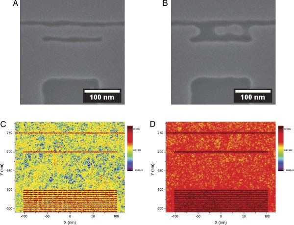
136                                       SCANNING VOL. 33, 3 (2011)

make it available to the scientific community as           Except for trivial cases, 3D structures are difficult to
performed with the previous versions (Hovington           build without visualization aids. In CASINO, the
et al., ’97; Drouin et al., 2007).                        creation of the 3D sample is helped by using the
   Two main challenges were encountered with the          OpenGL (http://www.opengl.org) technology to dis-
simulation of 3D samples: the creation of the 3D          play the sample and the display is also used when the
sample by the user and the slowdown inherent to the       simulation options are chosen. The 3D navigation
more complex algorithm needed for a true 3D               tool (rotation, translation, and zoom of the camera)
simulation. This article presents how we responded to     allows the user to assert the correctness of the sample
these challenges and goals. We also present the new       manually. In particular, the navigation allows the user
models and simulation features added to this version      to see inside the shape to observe imbedded shape.
of CASINO and examples of their applications.                Seven shapes are available in CASINO and they
                                                          are separate arbitrary in three categories. The first
                                                          category has only one shape, a finite plane. The finite
Features and Structure                                    plane is useful to define large area of the sample like a
                                                          homogenous film. However, the user has to be careful
   The simulation of electron transport in a 3D           that the plane dimension is larger than the electron
sample involves two computational aspects. The            interaction volume because the plane does not define
first one is the geometry computation or ray tracing       a closed shape and unrealistic results can happen if
of the electron trajectory inside the sample. For         the electron travels beyond the lateral dimensions of
complex geometry, the geometry computation can            the plane (Fig. 2(E) and next section). The second
involve a large effort (simulation time); hence, fast     category with two shapes contains 3D shape with
and accurate algorithms are needed. The second            only flat surfaces like a box. The box is often used to
aspect is the physical interaction with the matter        define a substrate. Also available in this category is
inside the sample. Both are needed to successfully        the truncated pyramid shape that is useful to simulate
simulate the electron trajectory.                         interconnect line pattern. The last category is 3D
   Using the electron transport 3D feature, the beam      shape with curved surface and contains four shapes.
and scanning parameters allow the simulation of           For these 3D shapes, the curved surface is approxi-
realistic line scans and images. From the simulated       mated by small flat triangle surfaces. The user can
trajectories, various distributions useful for analysis   specify the number of divisions used to get the
of the simulation are calculated. The type of dis-        required accuracy in the curved surface description
tribution implemented was driven by our research          for the simulation conditions. This category includes
need and various collaborations. Obviously, these         sphere, cylinder, cone, and rounded box shapes.
distributions will not meet the requirements of all          Complex 3D sample can thus be modeled by
users. To help these users use CASINO for their           using these basic shapes as shown in the examples
research, all the information from the saved electron     presented in this article.
trajectories, such as each scattering event position
and energy, can be exported in a text file for manual
processing. Because of the large amount of information
generated, the software allows the filtering of the        Regions
exported information to meet the user needs.
                                                             Each shape is characterized by two sides: outside
                                                          and inside. A region, which defines the composition
3D Sample                                                 of the sample, is associated to each side. The defini-
                                                          tion of outside and inside is from the point of view of
   The main aim of this work was to simulate more         an incident electron from the top (above the shape)
realistic samples. To achieve that goal, a 3D sample      toward the bottom (below the shape). The outside is
model was implemented in CASINO. Specifically,             the side where the electron will enter the shape. The
the Monte Carlo software should be able to build a        inside is the side right after the electron crosses the
3D sample and track the electron trajectory in a 3D       shape surface for the first time and is inside the shape.
geometry.                                                    The chemical composition of the sample is set by
                                                          regions. For each region, the composition can be a
                                                          single element (C) or multiple elements like a
Shapes                                                    molecule (H2O) or an alloy (AuxCu1x). For
                                                          multiple elements, either the atomic fraction or the
   The 3D sample modeling is performed by com-            weight fraction can be used to set the concentration
bining basic 3D shapes and planes. Each shape is          of each element. The mass density of the region can
defined by a position, dimension, and orientation.         be specified by the user or obtained from a database.
H. Demers et al.: 3D simulation with CASINO 137
For multiple elements region, the mass density is will always been selected when the electron inter-
calculated with this equation sects a triangle. The small gap is a lot smaller than
1 the electron mean free path, i.e. no collision occurs,
r ¼ P ci ð1Þ and the simulation results are not affected by the
n
i presence of the gap.
ri
Another type of ambiguity in the determination
where ci is the mass concentration and ri is the mass of the new region is shown in Figure 2(E) when an
density of element i. This equation assumes an ideal electron reaches another region without crossing
solution for a homogeneous phase and gives a any triangle boundaries. In CASINO, the change of
weight-averaged density of all elements in the sam- region occurs only when the electron trajectory
ple. If the true density of the molecule or alloy is cross a triangle boundary. As illustrated in
known, it should be used instead of the value given Figure 2(E), the region associated with an electron
by this equation. Also the region composition can inside the Au region define by the finite plane (the
be added and retrieved from a library of chemical dash lines define the lateral limit) and going out of
compositions. the dimension define by the plane, either on the side
For complex samples, a large number of material or top, does not change the region and the electron
property regions (two per shape) have to be speci- continue its trajectory as inside a Au region.
fied by the user; to accelerate the sample setup, the A typical 3D sample will generate a large number
software can merge regions with the same chemical of triangles, for example 106,082 triangles (6,240
composition into a single region. triangles per sphere) are required to model accu-
rately the tin balls sample studied in the application
section. For each new trajectory segment, the
Triangles and Mesh simulation algorithm needs to find if the electron
intersects a triangle by individually testing each
The change of region algorithm has been modified triangle using a vector product. This process can be
to allow the simulation of 3D sample. In the previous very intensive on computing power and thus time.
version, only horizontal and vertical layers samples To accelerate this process, the software minimizes
were available (Hovington et al., ’97; Drouin et al., the number of triangles to be tested by organizing
2007). An example of a complex sample, an the triangles in a 3D partition tree, an octree (de
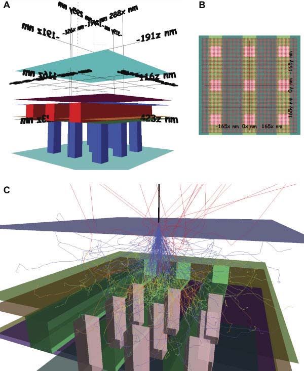
integrated circuit, is shown in Figure 1(A). Berg et al., 2008), where each partition is a box that
The electron trajectory ray tracing algorithm contains ten triangles. The search inside the parti-
(Akenine-Möller, ’97) does not work with the basic tions tree is very efficient to find neighbor partitions
shapes directly, but only with triangles. When the and their associated triangles. The engine generated
creation of the sample is finished, the software a new segment from the new event coordinate, see
transforms all the shape surfaces into triangles. electron trajectory calculation section. The ten tri-
Each triangle inherits the outside/inside material angles in the current partition are tested for inter-
properties of its parent shape. ception with the new segment. If not, the program
During the ray tracing of the electron trajectory, found the nearness partition that contains the new
the current region is changed each time the electron segment from the eight neighbor partitions and
intersects a triangle. The new region is the region created a node intersection event at the boundary
associated with the triangle side of emerging elec- between the two partition boxes. From this new
tron after the intersection. Figure 2(A) illustrates coordinate, a new segment is generated from the
schematically the electron and triangle interaction new event coordinate as described in the electron
and the resulting change of region. For correct trajectory calculation section. The octree algorithm
simulation results, only one region should be pos- allows fast geometry calculation during the
sible after an intersection with a triangle. This simulation by testing only ten triangles of the
condition is not respected if, for example, two tri- total number of triangles in the sample (106,082
angle surfaces overlap (Fig. 2(B)) or intersect triangles for the tin balls sample) and eight parti-
(Fig. 2(C)). In that case, two regions are possible tions; and generating the minimum of number of
when the electron intersects the triangle and if these new segments.
two regions are different, incorrect results can
occur. The software does not verify that this con-
dition is valid for all triangles when the sample is
created. The best approach is to always use a small Electron Trajectory Calculation
gap (0.001 nm) between each shape as shown in
Figure 2(D). No overlapping triangles are possible The Monte Carlo calculation scheme used in
with the small gap approach and the correct region CASINO is based on the previous version of138 SCANNING VOL. 33, 3 (2011) Fig 1. Screenshots from CASINO software of a 3D sample. (A) 3D view of the sample showing the different shapes and regions. (B) Top view of the sample with the scan points used to create an image. (C) Electron trajectories of one scan point with trajectory segments of different color for each region. The sample used is a typical CMOS stack layer for 32 nm technology node with different dielectric layers, copper interconnects, and tungsten via. CASINO (v2.42) (Drouin et al., 2007) and reviewed two elastic scattering events (Joy and Luo, ’89). It is in Joy’s book (Joy, ’95b). The detailed description of also possible to use a hybrid model for the inelastic the Monte Carlo simulation method used in the scattering where plasmon and binary electron– software is given in these references. In this electron scattering events are treated as discrete section, a brief description of the Monte Carlo events, i.e. just like the elastic event, and the rest of method is given and the physical models added or inelastic event is calculated with the mean energy modified to extend the energy range of the software loss model (Joy and Luo, ’89; Lowney, ’96). The are presented. calculation of each electron trajectory is performed The Monte Carlo method uses random numbers as follows. The initial position and energy of the and probability distributions, which represent the electron are calculated from the user specified elec- physical interactions between the electron and the tron beam parameters of the electron microscope. sample, to calculate electron trajectories. An elec- Then, from the initial position, the electron will tron trajectory is described by discrete elastic scat- impinge the sample, which is described using a tering events and the inelastic events are group of triangle surfaces (see previous section). approximated by mean energy loss model between The distance between two successive collisions is
H. Demers et al.: 3D simulation with CASINO        139

                                                                    in the energy range 10–500 keV. The calculations
                                                                    of the cross-sections used the default parameters
                                                                    suggested by the authors of the software ELSEPA
                                                                    (Salvat et al., 2005). These pre-calculated values
                                                                    were then tabulated and included in CASINO
                                                                    to allow accurate simulation of the electron
                                                                    scattering. The energy grid used for each element
                                                                    tabulated data was chosen to give an interpolation
                                                                    error less than 1% when a linear interpolation
                                                                    is used.
                                                                       A more accurate algorithm, using the rotation
                                                                    matrix, was added for the calculation of the direc-
Fig 2. Schema of the intersection of an electron trajectory         tion cosines. The implementation is based on the
and a triangle and the change of region associate with it.          MONSEL code (Lowney, ’95, ’96) from NIST.
(A) Single triangle where the new region is Au. (B) Two                The generation of SEs was added in CASINO
triangles overlap and ambiguity in the determination of the         using the hybrid energy loss model mentioned pre-
new region. (C) Intersection of two triangles with discontinuity    viously. The fast SEs are calculated using the Möller
in the determination of the new region. (D) Small gap approach
to resolve these two problems. (E) Another ambiguity in the         equation (Reimer, ’98). The slow SEs (SSE) are
determination of the new region (the red dash lines define the       generated from the plasmon theory (Kotera et al.,
lateral limit of the Au region of the plane shape).                 ’90). The implementation is based on the MONSEL
                                                                    code (Lowney, ’95, ’96) from NIST. To generate SE
obtained from the total elastic cross-section and a                 in a region, two parameters, the work function and
random number is used to distribute the distance                    the plasmon energies, are needed. Values for some
following a probability distribution. The elastic                   elements and compounds are included, but the user
scattering y angle is determined from another ran-                  can add or modify these values. The SSEs are low-
dom number and using the differential elastic cross-                energy electrons (o50 eV) and are very sensitive to
section calculated using analytical models or from                  the electron physical models and SE parameters
tabulated values. When the electron trajectory                      used. The modified Bethe equation with residual
intercept a triangle, the segment is terminated at the              energy constant is used to calculate the energy loss
boundary and a new segment is generated randomly                    at very low energy (o50 eV) (Lowney, ’96).
from the properties of the new region as described                     We did not validate the very low energy range
previously. The only difference is that the electron                (o50 eV) used in CASINO for the simulation of
direction does not change at the boundary. This                     SEs as the goal was to have a qualitative description
simple method to handle region boundary is based                    of secondary emission. We refer the user to the
on the assumption that the electron transport is a                  original article of each model for the validity of the
Markov process (Salvat et al., 2006) and past events                models.
does not affect the future events (Ritchie, 2005).
These steps are repeated until the electron either
leaves the sample or is trapped inside the sample,
which happens when the energy of the electron is                    Microscope and Simulation Properties
below a threshold value (50 eV). If the secondary
electrons (SEs) are simulated, the region work                         CASINO allows the user to choose various mi-
function is used as threshold value. Also, CASINO                   croscope and simulation properties to best match
keeps track of the coordinate when a change of                      his experimental conditions. Some properties greatly
region event occurs during the simulation of the                    affect the simulation time or the amount of memory
electron trajectory.                                                needed. These properties can be deactivated if not
   The tabulated values calculated from the ELSE-                   required.
PA cross-section software (Salvat et al., 2005) were                   The nominal number of simulated electrons is
added to CASINO. This electron elastic cross-                       used to represent the electron dose (with beam
section (EECS) model is also used by the Electron                   diameter) or beam current and dwell time. The
Elastic Scattering Cross Section Database                           simulation time is directly proportional to the
(Jablonski et al., 2003) available from NIST                        number of electrons. The shot noise of the electron
(Gaithersburg, MD). This EECS model involves the                    gun (Reimer, ’98) is included as an optional feature,
calculation of the relativistic (Dirac) partial-wave                which results in the variation of the nominal number
for scattering by a local central interaction poten-                of electrons N used for each pixel of an image or line
tial. The total and differential EECS were pre-                     scan. The number of electrons for a specific pixel
calculated using ELSEPA for all chemical elements                   Ni was obtained from a Poisson distribution PN
140 SCANNING VOL. 33, 3 (2011)
random number generator with: energy greater than 50 eV; an absorbed electron if
Ni
N N the electron is trapped inside the sample when the
PN ðNi Þ ¼ e : ð2Þ electron energy reaches below a threshold value (by
Ni !
default 50 eV); a TE if the electron exit the sample
Such features allows the user to study the impact of toward the bottom (same direction than the incident
the electron source which can greatly affect the electron). SE and PE that exit the sample with
results at low dose (o1,000e). energy less than 50 eV are used to calculate the
The SE feature is very demanding on computing secondary yield. If the energy is greater than 50 eV,
resource. For example, each 20 keV primary in- they are either a BSE or a TE depending on their
cident electron can generate a few thousands of SE exit direction.
electrons.
Three types of scan point distributions can be
used in the simulations: a single point, a line scan,
and an image. For all types, the positions are spe- Distributions for Each Scan Point
cified in 3D and a display is used to setup and draw
the scan points, see Figure 1(B), or alternatively The following distributions are used to under-
they can be imported from a text file. stand the complex interaction between incident
To manage the memory used in the simulation, electron and the sample.
the user can choose to keep or not the data (enabled The maximum penetration depth in the sample of
distributions, displayed trajectories) for each simu- the PE and BSE, the energy of BSEs when escaping
lated scan point. The cost of keeping all the data is the surface of the sample, the energy of the TEs
the large amount of memory needed during the when leaving the bottom of the thin film sample, the
simulation and the large file size. The main radial position of BSEs calculated from the primary
advantage is to have access to all the results for each beam landing position on the sample, and the
scan point which allows further post-processing. energy of BSE escaping area as a function of radial
For example, the energy absorption results pre- distance from the primary beam landing position
sented in Figure 7 needed 4 GB of memory during are distributions available in CASINO and
the simulation. described in detail elsewhere (Drouin et al., 2007).
The simulation of STEM image of amorphous A new distribution calculated for each scan point
sample is another important feature added to is the energy absorbed in a 3D volume. The volume
CASINO. The beam parameters now include the can be described in Cartesian, cylindrical, or sphe-
semi-angle and focal point, the energy range of rical coordinate. The 3D volume options are the
the physical models are extended up to 500 keV and position relative to the scan point, the size and
the transmitted electrons (TEs) are detected by an number of bins for each axis. To help choosing the
annular dark field (ADF) detector. These changes are 3D volume setting, a display shows the distribution
described in detail elsewhere (Demers et al., 2010). volume position and size relative to the sample.
Finally, the whole sample can be globally rotated Care must be taken when choosing the number of
in axial (Y) and/or azimuthal (Z) directions. The bins as the memory needed grows quickly. A typical
user should note that the rotation is applied simulation of energy absorbed can use 2 GB of
around the Y axis first, when values are given for memory for one scan point.
both directions.
Global Distributions
Distributions Calculated by CASINO
The following distributions either sum the con-
Two types of distributions are calculated by tribution of all scan points or compare the in-
CASINO. For the first, distributions are calculated formation obtained from each scan point.
for each scan point independently of the other scan The total absorbed energy distribution is the sum
points. For the second type, the distributions are of energy absorbed for all the electron trajectories of
obtained from the contribution of all scan points all scan points for a preset 3D volume. In this case,
either as a line scan or as an area scan (image). the 3D volume position is absolute, i.e. fixed relative
Before the description of these distributions, to the sample for all scan points.
some definitions used by CASINO are needed. The Intensity distributions related to line scan and
primary electron (PE) which is incident on the image are also calculated. The intensities calculated
sample is either at the end of the trajectory simu- are the BSE, SEs, absorbed energy, and TEs. The
lation: a backscattered electron (BSE) if the electron absorbed energy intensity is defined by the sum of
exits the sample toward the top direction and with all energies deposited by the electron trajectories inH. Demers et al.: 3D simulation with CASINO 141
the selected region for a given scan point. The can be saved as a high-intensity resolution TIFF
absorbed energy intensity signal will extend the scan image (32-bit float per pixel).
point position and will be limited by the interaction
volume. The intensity is either for the total number
of electrons simulated or normalized by the number Special Software Features
of electrons simulated. The intensity variation
between scan points is a combination of the shot The simulation of an image needs a large number
noise effect, if selected, and sample interaction. of scan points. Depending of the results selected, the
memory needed by CASINO can be large and exceed
the 2-GB limit of a 32-bit Windows system. Naturally,
the total simulation time increases with the number of
Representation of Collected Data scan points. For these reasons, CASINO uses multi-
processors/cores and can swap memory of a 32-bit
For the analysis of the distributions presented system. On a 64-bit system, there is no memory lim-
previously, it is useful to visualize the data directly in itation, so the software can use all memory available.
a graphic user interface before doing further proces- For the more advanced user requiring to investigate
sing using other software. In this section, the visua- the parameterization effect of one or a few simulating
lization aids available in CASINO are described. parameters a console version of CASINO is available
Figure 1(A) shows the user interface to create and with a basic scripting language. This feature allows the
visualize the sample in a 3D display. Figure 1(C) user to avoid to manually create a large numbers of
shows an example of electron trajectories simulated simulation setting using the graphical user interface
on sample shown in Figure 1(A). Through this which can be time consuming when one requires a
interface one can visualize the electrons interaction specific results such as the evolution of the BSE
with the sample. The color of the trajectories can be coefficient with the incident energy shown in Figure 3
used to represent the type of trajectory (not shown): for example. This feature allows the batch simulation
red for a BSE, green for a SE, and blue for the other of many simulations and to change one or more
electron (absorbed or transmitted). Another color parameters for each simulation. Also the console
scheme available allows to follow the regions in which version only uses portable C11 code, so that the
the electron go through, as shown in Figure 1(C), by software can be available on other operating systems
selecting the color of the electron trajectory segment like Linux and Mac OS X.
according to the region that contains it. Another
option for the visualization of the trajectory is to
represent the energy of the electron by different Application Examples
colors. Also the collision (elastic, inelastic, and change
of region events) that occurs along the trajectory can The following examples illustrate the application
be displayed with the help of small green sphere at the of the simulation tool in relation to BSE and SE
location of the collision (not shown). imaging, electron gun shot noise, and EBL.
The distributions obtained for all scan points are
displayed as 2D graphic if the scan points form a
straight line. In the case that the scan points form an
image, an intensity image is displayed with a color
bar mapped to the intensity value. The color scale
and minimum and maximum of the scale can be
specified by the user.
The signals or results obtained from the electron
simulation of all scan points that can be used to form
a line scan or an image are: the BSE, SEs, TE and the
absorbed energy inside the sample. For TE signal, the
user can choose to see the effect of the detector on the
intensity by using an ADF detector with user specified
semi-angles and detector quantum efficiency.
For most of the displays, the mouse allows to
change the zoom, translate, or rotate the informa-
tion presented. For all displayed graphics, the cor-
Fig 3. Simulated BSE coefficients Z in silicon at low electron
responding data can be exported/copied for further energy compared with experimental data (Bronstein and
analysis by the user or the graphic itself can be Fraiman, ’69; Joy, ’95a). 1,000,000 electrons were used in the
exported/copied. In addition, the intensity image simulations. BSE, backscattered electron.142 SCANNING VOL. 33, 3 (2011)
BSE Coefficient increases the simulation time by 20% vs. a linear
interpolation model.
The BSE coefficient Z is useful to validate the
Monte Carlo software. The Z value is the ratio of the
number of trajectories leaving the sample surface SE Yield
over all PE trajectories. The accuracy of Z depends
mainly on the electron elastic cross-section, the In a similar manner, the evolution of SE yield
energy loss models, and also the number of PE with the incident electron energy was used to vali-
simulated. The smooth variation of Z with incident date the SE generation implementation in CASINO.
electron energy helps identify problem with the Figure 4 compares the simulation of SE yields for
Monte Carlo implementation. the electron incident energy lower than 5 keV with
Figure 3 compares the simulation of BSE coeffi- experimental values (Bronstein and Fraiman, ’69;
cient for the electron incident energy lower than Joy, ’95a) for a silicon sample. The simulated values
5 keV with experimental values (Bronstein and are in agreement with the measured values except at
Fraiman, ’69; Joy, ’95a) for a silicon sample. The very low energy (less than 500 eV) where the simu-
simulated values are in agreement with the mea- lation and experimental values do not follow the
sured values except at very low energy (less than same trend.
500 eV) where the simulation and experimental The generation of SEs in the simulation increases
values do not follow the same trend. It is difficult to the simulation time drastically. For example, in bulk
assert the accuracy at very low energy of the simu- Si sample at 1 keV, the generation of SE increases
lation models from this difference. The experimental the simulation time by a factor of 17, and 44 at
values at these energies strongly depend on the 5 keV. For each PE trajectory, a large amount of SE
contamination or oxidation of the sample surface, trajectories are generated and simulated. For
which results in large variation of the values example at 1 keV, 100 SE trajectories are generated
obtained experimentally (Joy, ’95a). for each PE. The amount of SE trajectories increases
The linear interpolation problem reported in with more energetic PE, e.g. 1,300 SE trajectories
some Monte Carlo softwares (El Gomati et al., for each PE at 20 keV. The increase in the simula-
2008) was not observed in Figure 3. The inter- tion time is not directly proportional to the number
polated energy grid for the elastic electron cross- of SE trajectories, because, most of these new elec-
section data was chosen for each element to produce tron trajectories are low energy electron (SSE) and
an interpolation error less than 1% when a linear will have few scattering events, which take less time
interpolation model is used. This approach is similar to simulate than a PE.
to the one used in PENELOPE (Salvat et al., 2006).
The power law interpolation model proposed to
correct this problem (El Gomati et al., 2008) can Tin Balls Imaging
Another useful feature in CASINO is the ability to
simulate a set of scan points, e.g. a line scan or an
image. Figure 5 shows BSE and SE images simulated
with CASINO. The sample consists of Sn balls with
different diameters on a carbon substrate. Two different
incident electron energies were used 1 and 10 keV.
For each image, the contrast range was max-
imized to the minimum and maximum intensity of
the image. The contrast C was calculated to com-
pare the images using the following definition
(Goldstein et al., ’92)
S2 S1
C¼ ð3Þ
S2
where S1 and S2 are the minimum and maximum
pixel values in the image, respectively. These three
quantities are reported in Table I for each image.
At 1 keV, the contrast obtained with the BSE
Fig 4. Simulated SE yields d in silicon at low electron energy
compared with experimental data (Bronstein and Fraiman, signal is better than the SE signal, because the BSE
’69; Joy, ’95a). 100,000 electrons were used in the simula- emission has a stronger dependence on the atomic
tions. SE, secondary electron. number difference. For both signals, the smaller SnH. Demers et al.: 3D simulation with CASINO 143
Fig 5. Simulated images of tin balls on a carbon substrate. (A, B) BSE images. (C, D) SE images. The incident energy of 1 (A, C)
and 10 keV (B, D). The tin ball diameters are 20, 10, 5, and 2 nm. The field of view is 40 nm with a pixel size of 0.5 nm. The
nominal number of electrons for each scan point was 1,000. BSE, backscattered electron; SE, secondary electron.
TABLE I Comparison of the contrast values calculated from emission decreases by a factor 10 when the incident
BSE and SE images shown in Figure 5 for 1 and 10 keV energy increases from 1 to 10 keV. The decrease
incident electron energies does not change the contrast as both the carbon
Signal Energy (keV) Minimum Maximum Contrast substrate and Sn nanoparticle are similarly affected.
Again the decrease in the signal increases the effect
BSE 1 0.042 0.61 0.93 of the noise on the image resolution.
10 0.037 0.16 0.77
SE 1 0.61 2.9 0.79
The topographic information from the SE signal
10 0.063 0.35 0.82 is clearly observed in the large ball where the edges
are brighter than the center. The corresponding BSE
SE, secondary electron; BSE, backscattered electron. image in other hand looks flat and does not show
topographic information.
nanoparticles are visible, because the interaction These images are used to understand the impact
volume at 1 keV is of the order of few nanometers of microscope parameters on image resolution and
for both BSE and SE signals. At 10 keV, a similar features visibility.
contrast was obtained for BSE and SE images.
For BSE images, the contrast decreases with the
increase in incident energy. The larger interaction
volume decreases the signal from Sn nanoparticles Shot Noise Effect on Imaging
as less electron interaction occurs in the particle.
The decrease in the contrast at 10 keV increases the The number of electrons emitted by the electron
importance of the noise on the image resolution. gun is not constant, but oscillates around an average
The resolution changes drastically between the two value. This is the shot noise from the source and
energies. At 10 keV, the smaller tin balls (2 nm CASINO can include this effect in the simulation of
diameter) are not visible and the 5 nm diameter balls line scan or image.
are barely visible. Similar change in resolution are Figure 6 shows the effect of two different num-
observed on the SE images for the smaller tin balls bers of electrons on the BSE image quality. The
(2 nm diameter), but the 5-nm diameter balls sample is a typical microelectronic integrated circuit
are easier to see than on the BSE image. The SE shown in Figure 1(A). At 20 keV, the interaction144 SCANNING VOL. 33, 3 (2011)
Fig 6. Effect of the shot noise on the BSE images of integrated circuit ST sample. The nominal number of electrons for each scan
point was (A) 1,000 and (B) 10,000. The incident electron energy was 20 keV. The field of view is 700 nm with a pixel size of 10 nm.
BSE, backscattered electron.
volume reaches the copper interconnects, which are through the 50-nm resist film and 100-nm dielectric
buried 250 nm depth from the sample surface and film with little deviation. Most of the elastic collisions
increase the BSE emission. The presence of the occur in the Si substrate. However, the substrate
tungsten via will increase the BSE emission. The generates BSE that can emerge of the sample as far as
increase by the W via was barely observed in 4 mm from the beam impact. With a pattern com-
Figure 6(B) with 10,000 electrons, but not visible in posed of more than 225,000 scan points, the con-
Figure 6(A) with 1,000 electrons. The decrease in the tribution of the BSE on the absorbed energy cannot
nominal number of electrons from 10,000 to 1,000 be neglected. This is the background energy observed
illustrates the impact of the electron source noise on between patterns in Figure 7(C) and (D). The long
image quality. The shot noise feature in CASINO is range combined with the random nature of the BSE
useful to calculate the visibility of feature of interest exit position created a uniform and noisy back-
with different instrument parameters and feature ground signal. The average value of the absorbed
size. A detailed example of such study with CASINO energy background is proportional to the electron
is given elsewhere (Demers et al., 2010). dose. We suspect that for a specific value of the elec-
tron dose, the absorbed energy background reaches the
threshold value for the breakdown of the PMMA
molecule and development of the resist occurs outside
Energy Absorption in EBL
the expected patterns as observed in Figure 7(B).
However, this is just one possible explanation of the
The energy absorption feature of CASINO was failure. The electron exposure is only the first step of
used to study a problem encountered with EBL of a EBL. The resist development and profile evolution
pattern shown in Figure 7(A) and (B). Under cer- could be the source of the problem as well.
tain conditions, two close line patterns, separated
only by 50 nm, are connected after the development
of the resist. The sample consists of a 50-nm PMMA
film on a 100-nm thick SiO2 film with a Si substrate Conclusions
and the EBL was performed at 20 keV.
Monte Carlo simulations of the sample and pat- Improved simulation software for modeling sig-
tern were performed for two different electron doses nals generation in electron microscope from elec-
(number of electrons): 130 (33) and 700 mC/cm2 tron—sample interactions, which include a full 3D
(175). The total energy absorbed from the pattern sample geometry and an efficient 3D simulation
was calculated from the 3D matrix obtained with model, have been developed. All features are avail-
CASINO. Top view of the total energy absorption, able through a graphical user interface. It can be
normalized and on logarithmic scale, is shown in used for modeling BSE, SE, and TE signals and
Figure 7(C) and (D) for 130 and 700 mC/cm2 elec- absorbed energy, which is useful for EBL. The
trons doses, respectively. software features like scan points and shot noise
The expected patterns are clearly observed by allowing for the simulation and study of realistic
their dark grey (dark red online) color. The ab- experimental conditions. With the improved energy
sorbed energy in the pattern mainly comes from the range, this software can be used for SEM and
incident beam. At 20 keV, the electrons pass STEM applications, but with the limitation that theH. Demers et al.: 3D simulation with CASINO 145
Fig 7. Simulation of the electron dose effect on EBL. Two experimental SE images, after EBL, where the pattern was (A)
successfully developed and (B) incorrectly developed. (C, D) top view of the energy absorbed in the resist from the electron beam
pattern simulated with CASINO. The number of electrons per scan point was an: (C) electron dose of 130 mC/cm2 and (D)
electron dose of 700 mC/cm2. The energy absorbed is normalized and displayed on a logarithmic scale. SE, secondary electron;
EBL, electron beam lithography.
sample is considered as amorphous by the models References
and the simulation scheme used. The software
can be downloaded at this website: www.gel. Akenine-Möller T. 1997. A fast triangle-triangle intersection
test. J Graph Tools 2:25–30.
usherbrooke.ca/casino/index.html1 and used freely. Babin S, Borisov S, Ivanchikov A, Ruzavin I. 2006. Modeling
The software is in constant development for our of linewidth measurement in sems using advanced monte
research need and from user comments. carlo software. J Vac Sci Technol B 24:3121–3124.
Bronstein IM, Fraiman BS. 1969. Vtorichnaya elektronnaya
emissiya. Moskva: Nauka.
de Berg M, Cheong O, van Kreveld M, Overmars M. 2008.
Acknowledgements Computational geometry. Springer-Verlag.
Demers H, Poirier-Demers N, Drouin D, de Jonge N. 2010.
The authors greatly thank all the contributors to Simulating STEM imaging of nanoparticles in
micrometers-thick substrates. Microsc Microanal 16:
CASINO, in particularly R. Gauvin, P. Hovington, 795–804.
and P. Horny. Part of this version of CASINO was Ding ZJ, Li HM. 2005. Application of Monte Carlo simu-
developed with the help of John S. Villarrubia, lation to SEM image contrast of complex structures. Surf
Andras E. Vladar, and Mike Postek from NIST. Interface Anal 37:912–918.
Drouin D, Couture AR, Joly D, Tastet X, Aimez V,
EBL and SEM images were obtained at the Centre Gauvin R. 2007. CASINO V2.42—a fast and easy-to-use
de Recherche en NanoFabrication et en Nanocar- modeling tool for scanning electron microscopy and
actérisation (CRN2) research center at the microanalysis users. Scanning 29:92–101.
El Gomati MM, Walker CGH, Assa’d AMD, Zadrazil M.
Universite de Sherbrooke. This work was funded 2008. Theory experiment comparison of the electron
by NSERC. Research supported by NIH grant backscattering factor from solids at low electron energy
R01-GM081801 (to H.D, N.P.D., and N.J.). (250–5,000 eV). Scanning 30:2–15.
Gauvin R, Michaud P. 2009. MC X-ray, a new Monte Carlo
program for quantitative x-ray microanalysis of real
materials. Microsc Microanal 15:488–489.
Gnieser D, Frase CG, Bosse H, Tutsch R. 2008. MCSEM—a
1
If the link is invalid, a search with these two keywords should modular Monte Carlo simulation program for various
point out to the new location of the CASINO software: ‘‘Drouin applications in SEM metrology and SEM photo-
CASINO.’’ For obvious reason, the name of the program is not grammetry. In: Martina Luysberg KT, Weirich T, editors.
enough to find it. EMC 2008 14th European Microscopy Congress 1–5146 SCANNING VOL. 33, 3 (2011)
September 2008, Aachen, Germany. Springer: Berlin Lowney JR. 1996. Monte Carlo simulation of scanning
Heidelberg. p 549–550. electron microscope signals for lithographic metrology.
Goldstein JI, Newbury DE, Echlin P, Joy DC, Romig JAD, Scanning 18:301–306.
Lyman CE, Fiori C, Lifshin E. 1992. Scanning electron Newbury DE, Yakowitz H. 1976. Studies of the distribution
microscopy and x-ray microanalysis: a text for biologists, of signals in the SEM/EPMA by Monte Carlo electron
materials scientists, and geologists. New York: Plenum trajectory calculations: an outline. In: Heinrich KFJ,
Press. Newbury DE, Yakowitz H, editors. NBS Special Pub-
Hovington P, Drouin D, Gauvin R. 1997. CASINO: a new lication; October 1–3. National Bureau of Standards.
Monte Carlo code in C language for electron beam p 15–44.
interaction—Part I: description of the program. Scan- Reimer L. 1998. Scanning electron microscopy: physics of
ning 19:1–14. image formation and microanalysis. Berlin: Springer.
Jablonski A, Salvat F, Powell CJ. 2003. NIST electron Ritchie NWM. 2005. A new Monte Carlo application for complex
elastic-scattering cross-section database—version 3.1. sample geometries. Surf Interface Anal 37:1006–1011.
National Institute of Standards and Technology. Salvat F, Jablonski A, Powell CJ. 2005. ELSEPA—Dirac
Johnsen K-P, Frase CG, Bosse H, Gnieser D. 2010. SEM partial-wave calculation of elastic scattering of electrons
image modeling using the modular Monte Carlo model and positrons by atoms, positive ions and molecules.
MCSEM. Proceedings of SPIE. San Jose: California. Comput Phys Commun 165:157–190.
Vol. 7638.76381Op. Salvat F, Fernandez-Varea JM, Sempau J. 2006. PENE-
Joy DC. 1995a. A database of electron-solid interactions. LOPE-2006—a code system for Monte Carlo simulation
Scanning 17:270–275. of electron and photon transport. Facultat de Fisica
Joy DC. 1995b. Monte Carlo modeling for electron micro- (ECM), Universitat de Barcelona, Spain, Nuclear Energy
scopy and microanalysis. New York: Oxford University Agency.
Press. Villarrubia JS, Ding ZJ. 2009. Sensitivity of scanning electron
Joy DC, Luo S. 1989. An empirical stopping power relationship microscope width measurements to model assumptions.
for low-energy electrons. Scanning 11:176–180. J Micro/Nanolith MEM 8:033003–033011.
Kieft E, Bosch E. 2008. Refinement of Monte Carlo simu- Villarrubia JS, Ritchie NWM, Lowney JR. 2007. Monte
lations of electron–specimen interaction in low-voltage Carlo modeling of secondary electron imaging in three
SEM. J Phys D Appl Phys 41:215310. dimensions. Proceedingsof SPIE, Vol. 6518. San Jose:
Kotera M, Ijichi R, Fujiwara T, Suga H, Wittry DB. 1990. A California. p 65180K-1–65180K-14.
simulation of electron scattering in metals. Jpn J Appl Yan H, Gomati MME, Prutton M, Wilkinson DK, Chu DP,
Phys 29:2277–2282. Dowsett MG. 1998. Mc3D: a three-dimensional monte
Lowney JR. 1995. Use of Monte Carlo modeling for carlo system simulation image contrast in surface analytical
interpreting scanning electron microscope linewidth scanning electron microscopy. I—object-oriented software
measurements. Scanning 5:281–286. design and tests. Scanning 20:465–484.You can also read