Energetics of drop deformation with application to turbulence
←
→
Page content transcription
If your browser does not render page correctly, please read the page content below
This draft was prepared using the LaTeX style file belonging to the Journal of Fluid Mechanics   1

                                                              Energetics of drop deformation with
arXiv:2009.03962v2 [physics.flu-dyn] 29 Jan 2021

                                                                   application to turbulence
                                                                         Alberto Vela-Martı́n1,2 :, Marc Avila                  1
                                                   1
                                                       Center of Applied Space Technology and Microgravity (ZARM) University of Bremen, 28359
                                                                                                 Bremen
                                                            2
                                                              School of Aeronautics, Universidad Politécnica de Madrid, 28040 Madrid, Spain

                                                                                 (Received xx; revised xx; accepted xx)

                                                   Drop deformation in fluid flows is investigated here as an exchange between the kinetic
                                                   energy of the fluid and the surface energy of the drop. We show analytically that this
                                                   energetic exchange is governed only by the action of the rate-of-strain tensor on the
                                                   surface of the drop, more specifically, by a mechanism analogous to vortex stretching.
                                                   Our formulation allows to isolate the energetic exchange due to drop-induced surface
                                                   effects from the external action of turbulence fluctuations. We perform direct numerical
                                                   simulations of single drops in isotropic homogeneous turbulence and show that an
                                                   important contribution to the energetic exchange arises from the stretching of the fluid-
                                                   fluid interface by velocity fluctuations far from the drop surface. The identification of this
                                                   mechanism, which is approximately independent of surface dynamics in a wide range of
                                                   Weber numbers, sheds new light on drop deformation in turbulent flows, and opens the
                                                   venue for the improvement and simplification of breakup models.

                                                   Key words: turbulence, drop breakup, diffuse-interface methods

                                                   1. Introduction
                                                      The deformation of drops in turbulent flows is a key process in many natural phe-
                                                   nomena and industrial applications. Understanding the physical mechanisms that drive
                                                   this process is essential to develop accurate models to predict drop breakup (Hakansson
                                                   2019). Breakup models are necessary to predict the dynamics of binary mixtures and
                                                   the distribution of drop sizes, a relevant problem initiated with the seminal work of
                                                   Kolmogorov (1949) and Hinze (1955). Many commonly used models rely on an energetic
                                                   description of drop deformation, in which the surface energy of the drop increases due to
                                                   interactions with turbulent fluctuations until a maximum energy is reached and the drop
                                                   breaks. In particular, a widespread phenomenological picture describes drop deformation
                                                   and breakup as caused by the ‘impact’ of eddies on the surface of the drop (Andersson
                                                   & Andersson 2006). The kinetic energy of these eddies and their arrival frequency are
                                                   relevant model parameters, and an efficiency is usually introduced to account for an
                                                   incomplete energetic exchange in the process (see e.g. Lasheras et al. 2002; Liao & Lucas
                                                   2009, for reviews). This approach to modeling breakup is convenient because it lumps
                                                   the complexity of drop-turbulence interactions into model parameters, but it depends on
                                                   the validity of the model assumptions about the energetic exchange between the drop
                                                   and the turbulent flow.
                                                                    : Email address for correspondence: albertovelam@gmail.com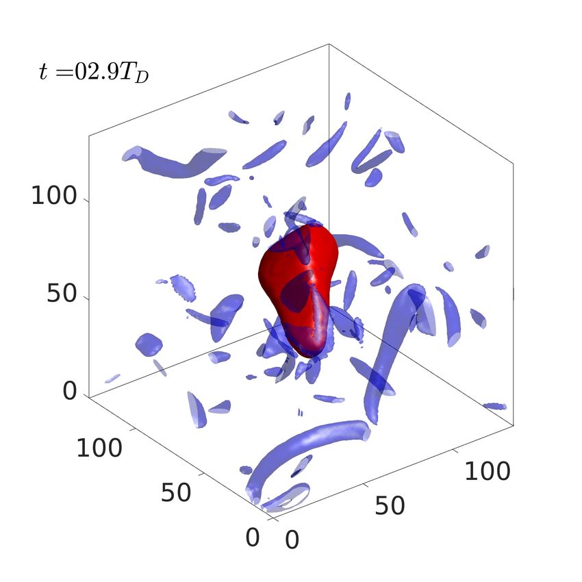
2                           Alberto Vela-Martı́n and Marc Avila
   Laboratory experiments to validate and to parametrise these (and other) models are
extremely challenging (see e.g. Risso & Fabre 1998; Eastwood et al. 2004; Maaß & Kraume
2012), hindering accurate predictions of drop breakup and drop-size distributions even
in simple turbulent flows (Aiyer et al. 2019). Direct numerical simulations have recently
provided quality data to study the energetics of drop-turbulence interactions (Dodd &
Ferrante 2016), but a poor understanding of the energy exchange mechanisms limits the
exploitation of these results for modelling.
   A convenient framework to analyze the energetic exchange between the kinetic energy
of the fluids and the surface energy of a drop (or more precisely the free energy of the
fluid mixture) is given by the Cahn–Hilliard–Navier–Stokes equations (Jacqmin 1999). In
these equations the interface is of finite thickness , but as  Ñ 0 the sharp-interface limit
is recovered (with the classical stress balance at the infinitesimal fluid-fluid interface, see
Magaletti et al. 2013). In this paper, we exploit this framework to show that this energetic
exchange is solely described by the action of the rate-of-strain tensor on the surface of
the drop. Moreover, this formulation allows to distinguish the self-induced increments
due to surface dynamics from the action of the surrounding turbulence. In this paper, we
leverage this approach to shed light on the mechanisms of drop deformation and breakup
in homogeneous isotropic turbulence.
   This paper is organised as follows. In §2, we present the derivation of the fundamental
mechanisms that drives the exchange between kinetic energy and surface energy. We
study this mechanism in direct numerical simulations of single drops, which are described
in §3. The results and their discussion are presented in §4 and §5. Finally, conclusions
are offered in §6.

2. Exchange between kinetic energy and surface energy
  We consider the incompressible Navier–Stokes (NS) equations coupled to the Cahn-
Hilliard (CH) equations,
                      ρpBt ui ` uj Bj ui q “ ´Bi p̃ ` 2Bj µSij ` fi ´ cBi φ,
                                                                                         (2.1)
                           Bt c ` uj Bj c “ κBkk φ,
which, together with the incompressibility constraint, Bi ui “ 0, describe the evolution of
an immiscible binary mixture of incompressible fluids (Jacqmin 1999). Here ui is the i-th
component of the velocity vector, p̃ is a modified pressure, Sij “ 12 pBi uj ` Bj ui q is the
rate-of-strain tensor and fi is a body-force term per unit volume. Repeated indices imply
summation, and we consider periodic boundary conditions. The concentration of each
component in the mixture is represented by c, where c “ ˘1 are the pure components.
The density, ρ, and the dynamic viscosity, µ, of the fluid mixture depend on c, and the
immiscibility is modeled through a chemical potential,
                                   φ “ βpc2 ´ 1qc ´ αBkk c.                              (2.2)
The true pressure is related to the modified pressure by p “ p̃`cφ´β{4pc2 ´1q2 `α{2pBi cq2
(Jacqmin 1999). The action of interfacial forces in the momentum equation is represented
by cBi φ, which is derived from physical energy-conservation arguments, and consistently
reproduces the linear relation between surface tension forces and the local curvature of
the interface (Jacqmin 1999). The numerical
                                         a      parameters α and β determine the typical
width of the fluid-fluid interface,  “ 4 2α{β, and the mobility, κ, determines its typical
relaxation time. When these parameters are fixed appropriately, κ „ 2 (Magaletti et al.
2013), the interface is consistently close to the equilibrium profile, ceq pxq “ tanh p4x{q,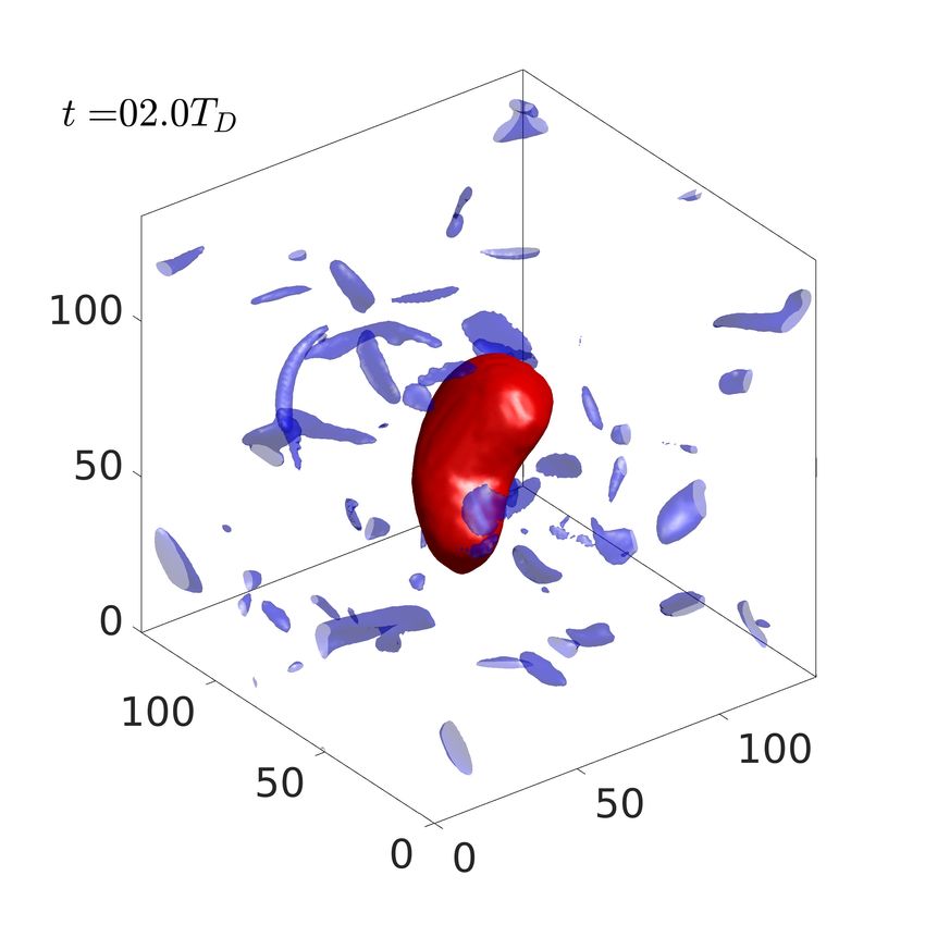
Energetics of drop deformation                               3
and the surface tension reads
                                    ż `8
                                           `         ˘2    4 a
                            σ“α                Bi ceq dx “ ?  αβ,                        (2.3)
                                     ´8                   3 2
where x is the spatial coordinate in the direction normal to the interface.

         2.1. Governing equations of the kinetic energy and the surface energy
  The evolution equation of the kinetic energy of the flow is obtained by taking the dot
product of the NS equations with ui . We consider that ´cBi φ “ φBi c ´ Bi pcφq, and the
second term in the right-hand side is absorbed into a new modified pressure, p1 “ p̃ ´ cφ.
Then the equation reads
              Bt e ` uj Bj e “ Bi pui p1 ` 2µuj Sij q ´ 2µSij Sij ` ui φBi c ` ui fi ,   (2.4)
where e “ 1{2ρui ui is the turbulent kinetic energy per unit volume. Considering periodic
boundary conditions, or in the absence of boundary fluxes, the only terms contributing
on average to the total kinetic energy budget are the local kinetic energy dissipation,
2µSij Sij , the power input, ui fi , and the energetic exchange between the kinetic energy
and the surface energy, φui Bi c. By multiplying the CH equation by the chemical potential,
we obtain,
                                    Bt h ` uj φBj c “ κφBkk φ,                           (2.5)
                 2     2             2
where h “ β{4pc ´ 1q ` α{2pBk cq is the free energy per unit volume. We now transform
(2.5) into an advection equation for h by decomposing the product φBi c and operating
on the partial derivatives. We find the relation
                                    φBi c “ Bi h ´ αBk τik ,                             (2.6)
where τik “ Bi cBk c is a Korteweg stress tensor. Substituting this expression in the kinetic
energy equation and the free energy equation, we obtain
                     Bt e ` uj Bj e “ Bi Ψi ´ 2µSij Sij ´ αui Bj τij ` ui fi ,
                                                                                         (2.7)
                     Bt h ` uj Bj h “ κφBkk φ ` αui Bj τij ,
where Ψi “ ui pp1 ` hq ` 2µuj Sij , and p1 ` h “ p ` αpBi cq2 . The free energy equation has
been transformed into an advection equation, where the first term in the right-hand side
represents the diffusive and dissipative action of the chemical potential, and the second
term the interaction of the fluid-fluid interface with the velocity field. This term describes
the action of a stress tensor, τij , and also appears in the kinetic energy equation.

              2.2. The physical mechanism of the surface energy variations
  The energy-exchange term can be further expanded into
                              αui Bj τij “ αBj pui τij q ´ αSij τij .                    (2.8)
The first term in the right-hand side represents the divergence of a flux and vanishes
in the mean for closed surfaces away from solid boundaries. Furthermore due to the
symmetric form of τij , only the symmetric part of the velocity gradient tensor, the rate-
of-strain tensor Sij , interacts with τij . Considering
                                                    a that the components of the vector
normal to the interface are ni “ Bi c{γ, where γ “ pBk cq2 , we rewrite the stress tensor as
τij “ ´αγ 2 ni nj , and the exchange term as ´αγ 2 ni Sij nj . This term describes the change
in free energy per unit volume; by integrating normal to the interface we transform it
into an energy change per unit surface,
                                         ϑ “ ´σni Sij nj .                               (2.9)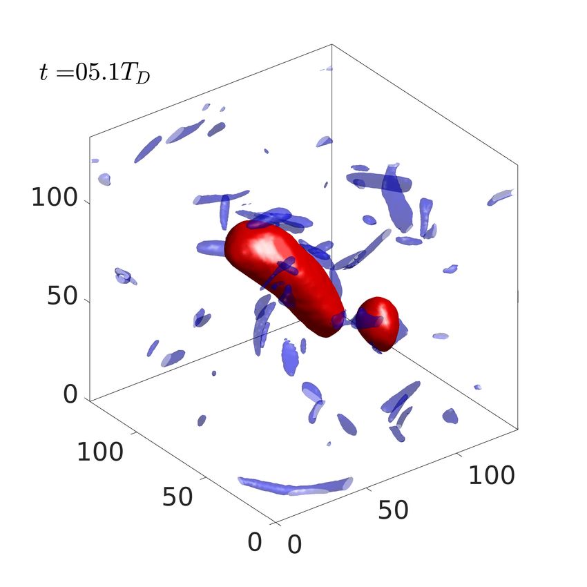
4 Alberto Vela-Martı́n and Marc Avila
(a) (b)
(c)
Figure 1. (a,b) Schematic representation of the mechanism that generates (a) positive and
(b) negative increments of the surface energy due to the compression or stretching of the drop
surface, where n is the orthogonal vector normal to the interface, t1 and t2 are vectors parallel to
the surface, and ϑ “ ´σni Sij nj . Blue and green arrows indicate the compressive and stretching
directions of the rate-of-strain tensor at the surface, and dotted lines are the streamlines of the
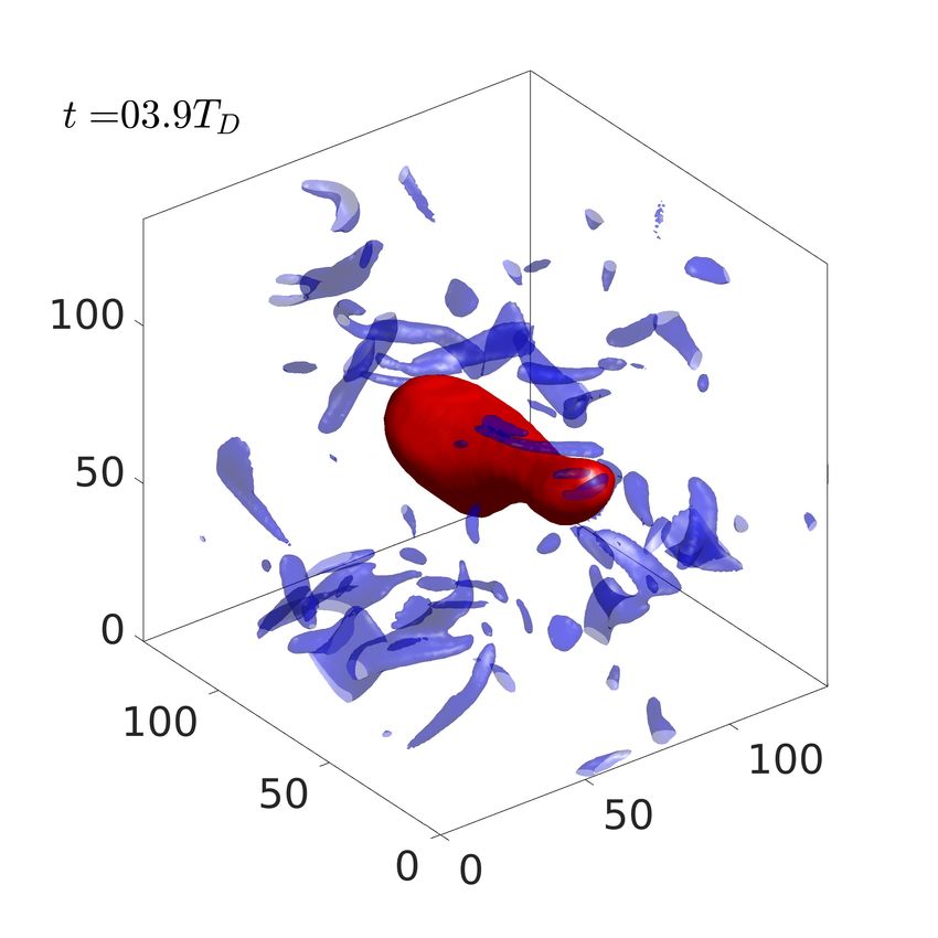
velocity field with respect to the surface. (c) Temporal evolution of a drop at We “ 1.8. The
frame is fixed at the center of the drop, and the time of the snapshots corresponds, from left
to right, to t{td “ 2.0, 2.9, 3.9, 4.8, and 5.1. Blue isosurfaces denote vorticity with magnitude
|ω| “ 2.6x|ω|y. The size of the computational box is marked in Kolmogorov units.
Here we have assumed that the interface is in equilibrium (so that eq. (2.3) holds) and
that neither n nor Sij change substantially across the interface width. Both assumptions
are fulfilled in the sharp-interface limit (Magaletti et al. 2013). The expression in (2.9)
resembles the vortex stretching term in the evolution equation of the enstrophy (squared
vorticity), which is responsible for the amplification of the vorticity vector. By analogy, ϑ
describes the stretching or contraction of the interface width by the rate-of-strain tensor.
This result may be difficult to interpret from a physical and geometrical perspective,
because the width of the interface between inmiscible fluids is of molecular scale, and
its relaxation time is much faster than the time-scale of the velocity gradients. In what
follows, we give this term a physical interpretation.
For simplicity and consistency with the numerical simulations shown later in this
paper, we have considered incompressible fluids. However the expression in (2.8), and
the subsequent analysis, holds regardless of the divergence of the velocity field. We have
only assumed that the gradients of the velocity field take place at a scale much larger than
the interface thickness. The expression in (2.9) is also valid for compressible flows as long
as the velocity field does not contain any discontinuity in the interface. Compressibility
modifies the energy equations in (2.7), since new fluxes and extra variables appear (in
particular the surface tension forcing terms added to the modified pressure must be
considered separately), but does not modify the structure of the exchange term, which
still remains the only net source of energy exchange. For the sake of generality we consider,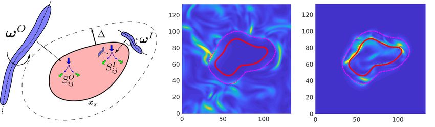
Energetics of drop deformation                               5
only in the following analysis, a compressible flow, and decompose the rate-of-strain
                                                            d
tensor into a deviatoric and a volumetric part, Sij “ Sij     ` P {3δij , where δij is the
Kronecker delta, and P “ Slk δlk is the local volumetric rate of expansion or contraction.
       d
Since Sij δij “ 0 and δij nj ni “ 1, we arrive at
                                          d
                             Sij nj ni “ Sij pnj ni ´ δij q ` P {3.                  (2.10)
Now we reformulate (2.9) in terms of P and of any pair of orthonormal vectors parallel
to the surface, t1 and t2 ,
                            ϑ “ σpt1k Skj
                                       d 1
                                          tj ` t2k Skj
                                                    d 2
                                                       tj q ´ σP {3,                 (2.11)
where we have considered that, nj ni ´ δij “ ´t1i t1j ´ t2i t2j . The first term represents
the growth rate of an infinitesimal surface area, δA, due to the deviatoric part of the
rate-of-strain tensor, which reads
                               1
                                 dt δA “ t1k Skj
                                              d 1
                                                 tj ` t2k Skj
                                                           d 2
                                                              tj .                 (2.12)
                              δA
The second term is related to compressibility effects, and is proportional to the growth
rate of an infinitesimal volume at the surface.
                                                                     d
  In the case of an incompressible flow, in which P “ 0 and Sij “ Sij  ,

                                 ϑ “ σpt1k Skj t1j ` t2k Skj t2j q,                  (2.13)
which shows that the surface energy increases as a consequence of the stretching of
the surface area by the rate-of-strain tensor. The opposite mechanism is also possible,
and the decrements of the surface energy are related to the contraction of the surface
area. In figure 1(a,b) we show a schematic representation of these mechanisms for an
incompressible flow. Hereafter, we limit our analysis to incompressible flows.
   By taking volume and surface averages of (2.7), we obtain an equation for the evolution
of the total kinetic energy and the total surface energy, E “ xeyV and H “ xhyV ,
                          dt H “ κxφBkk φyV ` xϑyS ,                                 (2.14)
                           dt E “ 2xµSij Sij yV ´ xϑyS ` xui fi yV ,                 (2.15)
where x¨yS denotes the integral over the fluid-fluid surface. On average, ϑ is the only
term responsible for the exchange of surface and kinetic energies. We stress that these
equations are valid independently of the physical properties of the fluids in the mixture.
Even in the case of different viscosities, the expression for ϑ remains valid and has
equal value at both sides of the interface. In this case, the balance of tangential stresses
produces a discontinuity in the rate-of-strain tensor (in the sharp-interface limit), but
this discontinuity only affects the off-diagonal components of the rate-of-strain tensor in
a frame fixed to the interface normal vector, which do not enter ϑ (Dopazo et al. 2000).

3. Single-drop experiments in homogeneous isotropic turbulence
   The analysis presented in the previous section is valid for any configuration of the
fluid-fluid interface, or flow regime. Hereinafter we apply our analysis to the dynamics of
a single drop embedded in a homogeneous and isotropic turbulent flow.

                                  3.1. Numerical method
  We consider two fluids with equal density and kinematic viscosity, and integrate (2.1)
in a triply periodic cubic domain of volume L3 “ p2πq3 by projecting the equations on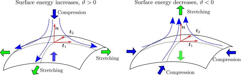
6                            Alberto Vela-Martı́n and Marc Avila
(a)                              (b)                              (c)
                                                                             10 -2
      6                                                                 4

      5                                10 0                             3

      4                                                                 2

      3                                                                 1

      2                                10 -5                            0

      1                                                                 -1

      0                                                                 -2
          2      4       6      8              0.1        1                          0.1   1

 Figure 2. (a) Median time to breakup as a function of the We. The upper and lower bars
 mark plus-minus the standard deviation. (b) Kinetic energy spectra at Reλ “ 58 for :                ,
 turbulent flow without droplet;          , We “ 1.8;         , We “ 5.4. Vertical dotted lines mark
 the scale (wavenumber) of the drop, kd “ 2π{d, the scale where the spectral density of the kinetic
 energy dissipation is the highest, kε , and the scale of the interface, k “ 2π{. (c) Pre-multiplied
 production spectra, kηΦpkq. Lines as in (a). The total contribution of each wavenumber to the
 variation of the surface free energy is represented as the area below the curve. Φ is normalized
 with its average in each case.

 a basis of N {2 Fourier modes in each direction, where N “ 256. Non-linear terms are
 computed through a dealiased pseudo-spectral procedure, and a third-order semi-implicit
 Runge-Kutta scheme is used for the time integration, with a decomposition of the linear
 terms proposed by Badalassi et al. (2003). To sustain turbulence in a statistically steady
 state, we implement a linear body-force, fpi “ Cf upi , that is only applied to wavenumbers
 k ă 2, where p̈ denotes the Fourier transform and k is the wavenumber magnitude. The
 forcing coefficient Cf is set so that, at each time, the total kinetic energy per unit time
 injected in the system is constant and equal to ε, while the kinematic viscosity ν “ µ{ρ
 is tuned to keep a prescribed numerical resolution, kmax η “ 4, where η “ pν{ε4 q3{4 is
 the Kolmogorov length scale and kmax “ N {3 is the maximum wavenumber magnitude
 after dealiasing.                                                          a
    The Reynolds numberaof the flow is Reλ “ λu1 {ν “ 58, where λ “ 15pν{εqu1 is the
 Taylor microscale, u1 “ 2E{3 is the root-mean-square of the velocity fluctuations, and
 E “ 1{2xui ui y is the ensemble-averaged kinetic energy. The thickness of the fluid-fluid
 interface is set by the Cahn number Ch “ pα{βL2 q1{2 “ 0.012, which for N “ 256 is
 appropriate to resolve the interface with a spectral Fourier  ? basis (Chen & Shen 1998).
 The mobility κ defines the Peclet number, Pe “ u1 L2 {κ αβ “ 3Ch´2 , which is fixed
 to ensure that the dynamics of the interface are consistent in the sharp-interface limit
 (Magaletti et al. 2013). The time-step is set to ∆t “ 0.04Ch. Simulations have been
 performed on GPUs using a modified version of the spectral code described in Cardesa
 et al. (2017). The code has been validated against Shao et al. (2018), and the consistency
 of the numerical parameters, such as the time-step and the spatial resolution, have been
 checked.

                              3.2. Initial conditions and drop size
    We introduce a drop of diameter d “ 31 L “ 45η in a fully developed turbulent
 flow, and integrate the governing equations (2.1) until the drop breaks. In figure 1(c),
 we show a visualization of a typical single-drop simulation. Since d " η, breakup is
 dominated by inertial forces and characterized by the Weber number, We “ ρε2{3 d5{3 {σ,
Energetics of drop deformation 7
and by a characteristic inertial time-scale td “ pd2 εq1{3 . To statistically characterise
drop deformation and breakup, we perform many independent single-drop simulations
initialized with statistically independent turbulent flow fields. Mass leakage (Yue et al.
2007) leads to a progressive reduction of the drop diameter, and to a time-dependent
Weber number, We : ptq, which decreases slightly through the simulations. However, this
variation is small, and therefore we do not employ any special numerical approach to
prevent it (Zhang & Ye 2017; Soligo et al. 2019). We consider the effective Weber number
of our simulations as the average Weber number at the average time of breakup, xtb y,
i.e We “ xWe : pxtb yqy. The difference between the time-dependent Weber number at the
time of breakup, We : ptb q, and the effective Weber number, We is at most „ 3% in the
worst cases.
We have performed simulations at four different effective We in the range of 1.8 ´
7.4. For each We the number of simulations is approximately 100, which yields a total
simulation time of between 300td and 1500td . From each simulation, we stored sufficient
full flow fields to have fully converged statistics. In figure 2(a), we show the median and
the standard deviation of the time to breakup, tb , as a function of the We. As expected,
lower values of the We yield longer times to breakup.
In what follows we show that although d is comparable to the integral scale of the flow,
the drop does neither modify the structure of the surrounding turbulence nor resonate
with the numerical box. The drop interacts mostly with scales smaller than d, indicating
that the linear forcing used to sustain turbulence does not affect breakup. In figure 2(b),
we show the average kinetic energy spectrum, Epkq “ 2πk 2 xp uup˚ yk , with and without an
immersed drop. Here x¨yk denotes averaging over modes with wavenumber magnitude k,
and ¨˚ represents the complex conjugate. The energy spectra is similar for the flow with
and without droplet above kη „ 1, indicating a physical turbulent structure in those
scales. To further corroborate this, we calculate the skewness and flatness factor of the
longitudinal velocity derivatives,
xpBi ui qn y
Fn “ , (3.1)
xpBi ui q2 yn{2
where no summation is intended for repeated indices. We find that, away from the drop
surface, F3 « ´0.52 and F4 « 5.2 independently of the Weber number, which are similar
to the values for a simulation without the drop and in the expected range for the Reλ
considered (Jiménez et al. 1993).
The good collapse of the energy spectra in the small wavenumbers (large scales) also
suggests the absence of any resonances between the drop and the box, which could
lead to spurious large-scale dynamics. To examine how the large-scale forcing affects the
dynamics of breakup, we study the pre-multiplied production spectra, kηΦpkq, shown in
figure 2(c), where
`{˘ ˚
Φpkq “ ´4πk 28 Alberto Vela-Martı́n and Marc Avila
(a) (b) (c)
Figure 3. (a) Decomposition of the rate-of-strain tensor acting on the drop surface in
O
contributions due to eddies a distance ∆ from the drop surface, denoted as Sij , and a distance
I
∆ closer to the surface and inside the drop, denoted as Sij . xs marks the drop surface. (b,c)
I I O O
Magnitude of the (b) inner and (c) outer rate-of-strain tensor, 2Sij Sij and 2Sij Sij , in a direct
numerical simulation for ∆ “ 9η and We “ 5.4. The solid red line marks the drop surface, and
the dashed magenta line a distance ∆ “ 9η from the surface. Axis in Kolmogorov units.
4. Analysis of the energetic exchange in isotropic turbulence
4.1. Local and non-local surface stretching
Despite the simplicity of the energetic exchange described in §2, the coupling between
the dynamics of the drop surface and the surrounding turbulence is bidirectional and
highly non-linear. The rate-of-strain tensor generates surface contraction or expansion,
and, at the same time, the surface dynamics generates straining motions. For instance,
as a deformed drop relaxes toward a spherical shape, the surface energy follows damped
oscillations before settling into equilibrium. Although these changes of the surface energy
are produced by the stretching and compression of the surface, they are drop-induced
and not necessarily related to drop breakup.
To separate the dynamics of the interface from the action of the surrounding tur-
bulence, we split the surface-stretching term into contributions related to eddies close
to, and inside the drop, and far from the drop. Here we consider eddies as patches
of swirling fluid, and associate them with the vorticity field. The kinematic relations
that hold between the vorticity vector and the rate-of-strain tensor imply that eddies
away from the drop stretch its surface by non-local effects (Ohkitani & Kishiba 1995;
Hamlington et al. 2008). We define the vorticity field at a distance ∆ from the drop
surface as
ω 1O “ Gpx; ∆qω, (4.1)
where ω “ ∇ ˆ u is the vorticity vector, and
Gpx; ∆q “ 1 if |x ´ xs |s ą ∆ and x P O,
(4.2)
Gpx; ∆q “ 0 if otherwise,
is a kernel that defines the region a distance ∆ from the drop surface. Here xs defines
the surface of the drop, |x ´ xs |s is the shortest Euclidean distance from x to the drop
surface, and O comprises all the points outside the drop. Let us note that ω 1O does not
define a vorticity field because it does not, in general, fulfill that ∇ ¨ ω O “ 0. We thus
project it into the closest divergence-free field, ω O “ ω 1O ´ ∇ψ, by solving
∇2 ψ “ ∇ ¨ ω 1O , (4.3)
with periodic boundary conditions. The stretching induced on the drop by the eddies
away from its surface can be calculated from the Biot–Savart law. By taking the curl ofEnergetics of drop deformation 9
(a) 1
(b) 0.2
0.8
0.15
0.6
0.1
0.4
0.05
0.2
0
0
-0.2 -0.05
0 2 4 6 8 10 2 3 4 5 6 7 8
Figure 4. (a,b) Correlation coefficient C between ϑI and ϑO as a function of (a) ∆ and (b)
We.
the vorticity and considering that ∇ ¨ uO “ 0, we obtain the following equation
∇2 uO “ ´∇ ˆ ω O , (4.4)
which, when solved with periodic boundary conditions, provides the rate-of-strain tensor
induced on the surface of the drop by eddies further and closer than ∆ from the drop
O
surface, Sij “ 21 pBj uO O I O
i ` Bi uj q and Sij “ Sij ´ Sij .
The stretching of the drop surface by eddies at distances larger than ∆ from the drop
surface is ϑO “ ´ni Sij O
nj , where the rate-of-strain tensor is evaluated at the surface of
I I
the drop, whereas ϑ “ ´ni Sij nj is the stretching induced on the surface by the flow
field inside the drop and at a distance smaller than ∆ from the drop surface. A schematic
representation of this decomposition and its application to a direct numerical simulation
are shown in figures 3(a)–(c).
4.2. Stretching by inner and outer eddies
We use here the decomposition presented in the previous section to separate the total
surface stretching into two contribution. First, a contribution due to eddies close to the
drop surface (or inside the surface) which are affected by surface dynamics or by the
material properties of the drop, and, second, another due to eddies far from the surface,
which are not affected by surface dynamics and independent of the material properties
of the drop. We call them ‘inner’ and ‘outer’ eddies respectively. In this section, we show
that in fact a separation in surface-driven, or ‘inner’, and surface-independent, or ‘outer’,
eddies takes place at a small distances (compared to the drop diameter) from the drop
surface.
A practical formal definition of the limit that separates inner and outer eddies is the
smallest ∆ for which the outer stretching is independent of surface dynamics, i.e when
there is not a coupled interaction between outer eddies and the surface. This definition
identifies the smallest region close to the drop surface affected by surface dynamics.
Since, as we will show in the following sections, ϑI is strongly influenced by surface
dynamics, we use the correlation coefficient between ϑO with ϑI evaluated at the drop
surface to quantify the independence of ‘outer’ eddies. The correlation coefficient is
defined as
xϑI ¨ ϑO y
C“b , (4.5)
2 2
I
xϑ yxϑ yO
where the bar denotes quantities without their average. We measure C for different We10 Alberto Vela-Martı́n and Marc Avila
(a) (b) (c)
10 0 10 0 10 0
-2 -2
10 -2 10 10
10 -4 10 -4 10 -4
10 -6 10 -6 10 -6
-10 -5 0 5 10 -10 -5 0 5 10 -10 -5 0 5 10
Figure 5. Probability density function of the local surface stretching due to (a) the full flow,
ϑ, (b) the inner eddies, ϑI , and (c) the outer eddies, ϑO , for ∆ “ 6η and at We “: , 1.8;
5.4. Quantities plotted without the mean and divided by their standard deviation.
and ∆, and present the results in figures 4(a,b). The correlation coefficient is close to
unity for ∆ „ 0, and decays fast with increasing ∆. For ∆ “ 6η, C « 0.2, and for ∆ “ 9η
it drops close to zero. As We decreases, the correlation coefficient increases slightly,
suggesting that the effect of surface dynamics on the surrounding eddies increases with
surface tension. These results suggest that ∆ between 6η “ 0.12d and 9η “ 0.19d is a
good approximation of the limit that separates ‘outer’ and ‘inner’ eddies, and that this
limit does not change substantially in the range of We considered here.
4.3. Statistics of the surface stretching
In figure 5(a)–(c), we show the probability density function (p.d.f) of ϑ, ϑO , and ϑI
measured at the surface of the drop for We “ 1.8 and 5.4, and for ∆ “ 6η “ 0.13d.
We find that ϑ and ϑI are very similar and display fairly fat-tailed distributions which
depend on the We. On the other hand, the p.d.f’s of ϑO are more symmetric, closer
to a Gaussian. The good collapse of the pdf’s at two different We suggests that the
surface stretching produced by eddies a distance further than ∆ “ 6η “ 0.13d from
the drop is not affected by surface dynamics. These results are qualitatively similar for
∆ “ 9η “ 0.19d.
In figure 6(a), we show the mean of ϑ, ϑO , and ϑI normalised with ρu3d , where ud “
d{td , for different values of We and ∆. The average of ϑ increases with We, which is
consistent with the statistics of the breakup time. Assuming that the breakup of an
initially spherical drop takes place when a critical increment of the surface energy is
reached, ∆Hb (Andersson & Andersson 2006), and that the surface energy can only
increase due to the stretching term, its average measured on the surface of the drop is
related to the time to breakup by
@ ∆Hb D
tb „ , (4.6)
ϑd2
which has been estimated by averaging equation (2.14) in time, considering that xϑyS „
xϑyd2 , and neglecting the dissipation of surface energy. As W e decreases, the time to
breakup increases (figure 2(a)), and xϑy decreases.
For ∆ “ 6η and ∆ “ 9η, the average contribution of the outer eddies to the stretching
of the interface is larger than, or at least comparable to, the inner contribution, and
this contribution changes only slightly with the We. Conversely, the inner contribution
increases substantially with We, transitioning from xϑI y ă 0 at low We to xϑI y ą 0 atEnergetics of drop deformation 11
(a) (b)
10 -2
15
10
5
10 0
0
-5
-10
10 -1
2 3 4 5 6 7 8 2 3 4 5 6 7 8
(c) (d)
0 8
-0.1
6
-0.2
-0.3
4
-0.4
-0.5 2
-0.6
-0.7 0
2 3 4 5 6 7 8 2 3 4 5 6 7 8
Figure 6. (a) Mean, (b) standard deviation, (c) skewness and (d) excess flatness of ϑ as a
function of We. Mean and standard deviation normalized with ρu3d , where ud “ d{td . Solid
symbols corresponds to the statistics of ϑO , and empty symbols to ϑI . Color lines correspond
to ∆ “: , 6η; , 9η; and solid black line to the full rate-of-strain tensor. In (b) the
dotted line is proportional to We ´1 .
high We. This transition takes place at approximately We „ 3.5, and will be examined
in §4.5.
In figure 6(b), we show the standard deviation of ϑ normalised with ρu3d . It is approx-
imately proportional to We ´1 , and substantially higher for the inner than for the outer
contributions. In all cases, the standard deviation of the local surface stretching is larger
than its mean, and this difference becomes particularly significant as We decreases. These
results suggest that a very significant part of the stretching is not efficient, and cancels
out when averaging, specially for the inner stretching and for small Weber numbers.
We focus now on higher order statistics of the surface stretching, in particular in the
skewness and the flatness factor, which are defined as
Fn pϑq “ xpϑ ´ xϑyqn y{xϑ2 ´ xϑy2 yn{2 , (4.7)
for n “ 3, and n “ 4 respectively, and are shown in in figures 6(c,d). For ease of
reference, we consider the so-called excess flatness factor, i.e the flatness factor minus
that of a Gaussian distribution, for which F4 “ 3. These statistical moments emphasize
the strong distinction between inner and outer stretching. While the skewness of the outer
contributions is close to zero and does not change with We, the statistics of the inner
stretching are more negatively skewed, and show dependence with We. The flatness factor
conveys a similar picture. The outer contributions have a low, We-independent, flatness
factor, whereas for the inner contributions the flatness factor increases substantially with12 Alberto Vela-Martı́n and Marc Avila
(a) (b)
2 2
1.5 1.5
1 1
0.5 0.5
0 0
0 0.2 0.4 0.6 0.8 1 0 0.2 0.4 0.6 0.8 1
(c) (d) 3
2
2.5
1.5 2
1.5
1
1
0.5
0.5
0 0
0 0.2 0.4 0.6 0.8 1 0 0.2 0.4 0.6 0.8 1
Figure 7. (a)-(c) Probability density function of cos θi “ n ¨ v i , where v i are the principal
directions of the rate of strain tensor and λ1 ď λ2 ď λ3 are their eigenvalues. Solid markers
correspond to angles calculated with the inner flow field, and empty markers to the outer field
for ∆ “ 9η. (d) Similar but for the vorticity vector of the full flow field, cos θω “ n ¨ ω{|ω|. Lines
correspond to We “: , 1.8; , 3.6; , 5.4. The vertical dotted line in (a) and (c)
marks cos π{4.
decreasing We. These results corroborate, first, that the statistics of the outer stretching
are roughly We-independent, as anticipated by the remarkable collapse in figure 5(c),
and, second, that the inner stretching has an intermittent structure, with intense events
of ϑ becoming stronger with decreasing We.
4.4. Geometrical characterization of the inner and outer stretching
To further explain the statistical differences between the inner and outer contributions,
and their dependence with We, we study the structure of the rate-of-strain tensor induced
by inner and outer eddies, and of the vorticity vector, on the surface of the drop. In the
spirit of the analysis of vortex stretching in isotropic turbulence (Ashurst et al. 1987),
we analyse the surface stretching term in the frame of reference of the eigenvectors of
the rate-of-strain tensor, and quantify the contribution of each of its eigenvalues to the
total stretching of the drop surface.
In figure 7(a)–(c), we show the p.d.f of the cosine of the angle of alignment between
each of the principal axes of the rate of strain tensor, v 1 , v 2 and v 3 (where λ1 ď λ2 ď λ3
are their corresponding eigenvalues) and the normal to the surface, n. For the inner
contributions, the most stretching (v 3 ) and the most compressing (v 1 ) eigenvectors tend
to be oriented at „ 45o with respect to the surface normal, and therefore also to the
surface tangent plane, while the intermediate eigenvalue is predominantly normal to the
surface normal (parallel to the surface tangent plane). As shown in figure 7(d), also theEnergetics of drop deformation 13
(a) (b)
0.3
0.1
0.2
0.1 0.05
0 0
-0.1 -0.05
-0.2
-0.1
-0.3
-0.15
2 3 4 5 6 7 2 3 4 5 6 7
(c) (d)
5 10 0
4
3 10 -1
2
1 10 -2
2 3 4 5 6 7 8 -1 -0.5 0 0.5 1
Figure 8. (a,b) Average surface stretching due to each eigenvalue of the rate-of-strain tensor,
pi “ σλi sin2 θi as a function of the Weber number for the inner (a) and the outer (b)
contributions, for ∆ “ 9η. Surface stretching normalised with ρu3d . (c) Surface average of the
I I
square of the inner rate-of-strain tensor, 2Sij Sij , for ∆ “ 9η, and the vorticity vector ωi ωi for
different Weber numbers, normalised with Kolmogorov units. (d) p.d.f of Λ “ log2 |λ1 |{λ3 for
different Weber numbers.
vorticity vector aligns strongly normal to n, and parallel to the surface. This tendency
was also reported by Soligo et al. (2020). In all cases, the alignment is more marked for
small We, revealing an important effect of surface dynamics on the configuration of the
velocity gradients at the surface.
The outer contributions to the stretching of the surface show a substantially different
picture. There is a consistent tendency of the most compressing eigenvector to align
normal to the surface, and of the most stretching to align parallel to it, although the
alignment is less marked than for the inner rate-of-strain tensor. The good collapse at
different We suggests that this effect is roughly independent of the surface dynamics.
We further decompose the surface stretching term into the contribution of each of its
eigenvalues. A possible approach is to consider the rate of compression or stretching of
the vector normal to the surface by each eigenvalue, ri “ ´σλi sin θi (no summation for
repeated indices is intended), which yields
ϑ “ r1 ` r2 ` r3 “ ´σpλ1 cos2 θ1 ` λ2 cos2 θ2 ` λ3 cos2 θ3 q. (4.8)
However this decomposition cannot be readily interpreted from a physical perspective.
Instead, we consider the contribution of each eigenvalue to the stretching or compression
of the surface tangent plane, pi “ σλi sin2 θi . Note that sin θi “ cospπ{2 ´ θi q is the
projection of each eigenvector on the surface tangent plane. Since λ1 ` λ2 ` λ3 “ 0, and14 Alberto Vela-Martı́n and Marc Avila
cos2 θi “ 1 ´ sin2 θi , the total surface stretching reads,
ϑ “ p1 ` p2 ` p3 “ σpλ1 sin2 θ1 ` λ2 sin2 θ2 ` λ3 sin2 θ3 q. (4.9)
In figures 8(a,b), we show the averages of pi for the inner and outer contributions. In
both cases the surface stretching and compression due to p1 and p3 is much larger in
absolute value than that of p2 (note that in the plot p1 and p3 are divided by 10 for ease
of visualization). However, there is a significant cancellation between p1 and p3 , so that
xp1 ` p3 y „ xp2 y.
For the outer contribution, p1 `p3 produces net surface stretching, which can be traced
to the tendency of v 3 to align parallel to the surface (or v 1 normal to it), and p2 does
not play a relevant role in the average stretching. This is in agreement with the almost
random orientation of v 2 with respect to the surface normal, as shown in figure 7(b).
For the inner contributions, the cancellation of p1 and p3 is consistent with a predom-
inant alignment of v 1 and v 3 at „ 45o with respect to the normal and to the surface
tangent plane. In this case, p2 contributes substantially to the average stretching of the
surface. As We increases, the absolute value of xp1 `p3 y decreases, and xp2 y progressively
dominates the average stretching, explaining the transition from xϑI y ă 0 to xϑI y ą 0 as
We increases.
4.5. Transition from a 2D to a 3D structure of the rate-of-strain tensor
We focus now on the intensity and structure of the velocity gradients at the drop
I I
surface. In figure 8(c), we show the average of 2Sij Sij for ∆ “ 9η, and ωi ωi , measured
at the surface of the drop. Although the surface dynamics increases the intensity of the
velocity gradients on the surface of the drop with decreasing We, surface tension forces
impose a strong constraint on their structure. The constraint of the velocity gradients is
very noticeable in the rate-of-strain tensor, which has a quasi-2D structure at low We,
with |λ2 | ! |λ3 | « |λ1 |, and becomes progressively 3D as We increases. To characterise
this process we analyse
|λ1 |
Λ “ log2 , (4.10)
λ3
at the drop surface. Since 12 λ3 ď |λ1 | ď 2λ3 , this quantity is defined in the range
´1 ď Λ ď 1. Predominant Λ ą 0 is characteristic of fully developed 3D turbulence,
and implies that λ2 ą 0 on average, while Λ “ 0 indicates 2D dynamics, in which
λ1 “ ´λ3 and, by continuity, λ2 “ ´λ1 ´ λ3 “ 0. As shown in figure 8(d), the p.d.f
of Λ shows that, for small We, |λ1 | „ λ3 and λ2 „ 0, and that, on average, λ2 grows
positive as We increases, indicating a transition from a quasi-2D to a 3D structure of
the rate-of-strain tensor at the surface. As λ2 increases with respect to λ3 and |λ1 |, the
net stretching that it produces on the surface becomes more relevant, and, as shown in
the previous section, xp2 y dominates over xp1 ` p3 y, leading to xϑI y ą 0.
5. Discussion
We have separated the total stretching of the drop surface in contributions from
inner and outer eddies. For distances to the drop surface larger than ∆ ą 6η, the
two contributions are not correlated pointwise (figure 4), indicating that outer eddies
are independent of surface dynamics. This is corroborated by the statistics of the outer
surface stretching, which are roughly We-independent. The surface stretching due to
outer eddies contributes on average to the increment of the surface energy at all We, andEnergetics of drop deformation 15 its statistics do not depend strongly on We, which implies that they depend mostly on the structure of the surrounding turbulence. For low We, the surface dynamics produces a net energy flux from the surface energy to turbulent kinetic energy, while for large We, the inner eddies tend to stretch the surface on average, increasing the surface energy. In all cases, the inner surface stretch- ing term shows strongly intermittent and negatively-skewed We-dependent statistics. Intense negative events of the surface stretching become more relevant as We decreases, evidencing the enhanced ability of the surface to restore the deformations caused by turbulent fluctuation, and transferring the surface energy back to turbulent fluctuations. By conservation, this energy is on average dissipated by the flow. In this low-We scenario, the net increments of the total surface energy depend on the interplay between outer surface stretching and the ability of the surface to transfer energy through inner eddies into turbulent fluctuations. By analysing the structure of the inner velocity gradients on the surface of the drop, we have shown that at low We the rate-of-strain tensor is strongly controlled by surface tension forces. Although its average magnitude is larger than in the turbulent background, providing enhanced dissipation of turbulent kinetic energy, its 2D structure and its configuration with respect to the interface precludes the net stretching of the surface. As We increases and surface tension forces become less dominant, the rate-of-strain tensor develops a 3D structure in which its intermediate eigenvalue becomes predominantly positive, producing net stretching of the surface. This phenomenon explains the transition from a negative to a positive average contribution of the inner eddies to the total surface stretching. We have reported a statistically significant alignment of the surface normal with the most compressing direction of the outer rate-of-strain tensor, and of the surface tangent plane with the most stretching one. This phenomenon, which is also observed in the evolution of passive material surfaces in turbulence, and naturally leads to this configuration (Girimaji & Pope 1990), indicates the persistent stretching of the drop surface by outer eddies. The similar statistics of the alignment angles in a wide range of We suggests that this mechanism is rather independent of surface dynamics. The stretching by outer eddies is a plausible mechanism for drop deformation, with the exception that the drop surface interacts with the fluid, and resists deformation. 6. Conclusions In this work we have analysed the energetics of fluid-fluid interfaces. Our main con- tribution is to provide a mathematical description of the mechanism responsible for the energetic exchange between the kinetic energy of the flow and the surface energy of the fluid-fluid interface. We have shown that this exchange occurs due to the stretching or compression of the surface area by the rate-of-strain tensor. There result stress the relevant role of straining motions in drop deformation and breakup, in agreement with experiments and theoretical analyses of laminar flows in the Stokes limit (Rallison 1984). We have separated the total stretching into contributions due to inner and outer eddies. We use here the term outer to refer to eddies sufficiently far from the drop surface for their dynamics to be unaffected by surface tension forces. Conversely, we define inner eddies as those close to the surface or inside the drop, whose dynamics are affected either by surface tension forces or by the material properties of the fluid inside the drop. The stretching of the drop surface by outer eddies contributes substantially to the total surface energy budget. This mechanism constitutes a quantitative reinterpretation of the ‘collision’ of eddies (Andersson & Andersson 2006).
16                         Alberto Vela-Martı́n and Marc Avila
   We have shown that the surface stretching due to inner and outer eddies are locally
uncorrelated, indicating that these terms may be considered separately. A ‘random’ ap-
proach to breakup modelling appears to be justified since outer eddies are, by definition,
not coupled to the dynamics of the interface, precluding any synergies that may lead
to enhanced breakup (at least in the simple case of equal density and viscosity). An
interesting question is how this analysis applies to bubbles, for which their characteristic
oscillatory frequency seems to play a relevant role in breakup (Risso & Fabre 1998). In
drops, deformation and breakup necessarily occurs as an interplay between inner and
outer dynamics, but we suggest that the latter may be the driver of the process. In the
context of drop deformation and breakup, our results pave the way for a better under-
standing of this phenomenon from an energetic perspective, and provide a consistent
quantitative framework to tune, improve and develop breakup models.
   Although our study is limited to the ideal case of incompressible fluids with equal
density and viscosity, the theoretical analysis in §4 applies equally to compressible fluids,
and to fluid pairs with different viscosity and density. In the latter case, we expect the
contribution of inner dynamics to change considerably. For instance, we suggest that an
increment of the drop viscosity substantially affects the inner dynamics due, first, to
the kinematic relations imposed on the rate-of-strain tensor across the interface, which
depend on the viscosity ratio (Dopazo et al. 2000), and second, by the enhanced ability of
the fluid inside the drop to diffuse momentum and dissipate energy. These changes may
inhibit the stretching of the surface by inner eddies and/or provide a fast mechanism to
dissipate the surface energy produced by the stretching of outer eddies, explaining the
resistance of viscous drops to breakup (Calabrese et al. 1986; Roccon et al. 2017).
   An important question that we have partially addressed in this work is whether breakup
occurs as a progressive buildup of surface energy due to the accumulative interaction with
many eddies, or as sharp increments of the surface energy due to interaction with isolated
intense turbulent events. Although answering this question necessarily requires temporal
analysis, we have shown that the standard deviation of the local surface stretching is
much larger than its mean, possibly reflecting inefficient stretching that cancels out.
These results point in the direction of the second scenario. A tentative picture is that
weak background turbulence produces much of this inefficient stretching, whereas the
interaction with just a few of the most intense turbulent structures produces the effective
stretching leading to breakup.

Acknowledgements
 A.V-M acknowledges the support of the European Research Council COTURB project
ERC-2014.AdG-669505.

Declaration of interest
  The authors report no conflict of interest.

                                      REFERENCES
Aiyer, A.K., Yang, D., Chamecki, M. & Meneveau, C. 2019 A population balance model
     for large eddy simulation of polydisperse droplet evolution. J. Fluid Mech. 878, 700–739.
Andersson, R. & Andersson, B. 2006 On the breakup of fluid particles in turbulent flows.
     AIChE Journal 52, 2020–2030.
Ashurst, W.T., Kerstein, A.R., Kerr, R.M. & Gibson, C.H. 1987 Alignment of vorticity
Energetics of drop deformation 17
and scalar gradient with strain rate in simulated navier–stokes turbulence. Phys. Fluids
30, 2343–2353.
Badalassi, V.E., Ceniceros, H.D. & Banerjee, S. 2003 Computation of multiphase systems
with phase field models. J. Comput. Phys. 190, 371–397.
Calabrese, R.V., Chang, T.P.K. & Dang, P.T. 1986 Drop breakup in turbulent stirred-tank
contactors. Part I: Effect of dispersed-phase viscosity. AIChE J. 32, 657–666.
Cardesa, J.I., Vela-Martı́n, A. & Jiménez, J. 2017 The turbulent cascade in five dimensions.
Science 357, 782–784.
Chen, L.Q. & Shen, J. 1998 Applications of semi-implicit fourier-spectral method to phase
field equations. Comput. Phys. Commun. 108, 147–158.
Dodd, M.S. & Ferrante, A. 2016 On the interaction of taylor length scale size droplets and
isotropic turbulence. J. Fluid Mech. 806, 356–412.
Dopazo, C., Lozano, A. & Barreras, F. 2000 Vorticity constraints on a fluid/fluid interface.
Phys. Fluids 12, 1928–1931.
Eastwood, C.D., Armi, L. & Lasheras, J.C. 2004 The breakup of immiscible fluids in
turbulent flows. J. Fluid Mech. 502, 309–333.
Girimaji, S.S. & Pope, S.B. 1990 Material-element deformation in isotropic turbulence. J.
Fluid Mech. 220, 427–458.
Hakansson, A. 2019 Emulsion formation by homogenization: Current understanding and future
perspectives. Annu. Rev. Food Sci. Technol. 10, 239–258.
Hamlington, P.E., Schumacher, J. & Dahm, W.J.A. 2008 Local and nonlocal strain rate
fields and vorticity alignment in turbulent flows. Phys. Rev. E 77 (2), 026303.
Hinze, J.O. 1955 Fundamentals of the hydrodynamic mechanism of splitting in dispersion
processes. AIChE Journal 1 (3), 289–295.
Jacqmin, D. 1999 Calculation of two-phase Navier–Stokes flows using phase-field modeling. J.
Comput. Phys. 155, 96–127.
Jiménez, J., Wray, A., Saffman, P.G. & Rogallo, R.S. 1993 The structure of intense
vorticity in isotropic turbulence. J. Fluid Mech. 255, 65–90.
Kolmogorov, A.N. 1949 On the disintegration of drops in turbulent flow. In Doklady Akad.
Nauk. USSR, , vol. 66, p. 825.
Lasheras, J.C., Eastwood, C., Martınez-Bazán, C. & Montanes, J.L. 2002 A review of
statistical models for the break-up of an immiscible fluid immersed into a fully developed
turbulent flow. Int. J. Multiph. Flow 28, 247–278.
Liao, Y. & Lucas, D. 2009 A literature review of theoretical models for drop and bubble
breakup in turbulent dispersions. Chem. Eng. Sci. 64, 3389–3406.
Maaß S. & Kraume, M. 2012 Determination of breakage rates using single drop experiments.
Chem. Eng. Sci. 70, 146 – 164.
Magaletti, F., Picano, F., Chinappi, M., Marino, L. & Casciola, C. M. 2013 The sharp-
interface limit of the Cahn–Hilliard/Navier–Stokes model for binary fluids. J. Fluid Mech.
714, 95–126.
Ohkitani, K. & Kishiba, S. 1995 Nonlocal nature of vortex stretching in an inviscid fluid.
Phys. Fluids 7, 411–421.
Rallison, J.M. 1984 The deformation of small viscous drops and bubbles in shear flows. Annu.
Rev. Fluid Mech. 16, 45–66.
Risso, F. & Fabre, J. 1998 Oscillations and breakup of a bubble immersed in a turbulent field.
J. Fluid Mech. 372, 323–355.
Roccon, A., De Paoli, M., Zonta, F. & Soldati, A. 2017 Viscosity-modulated breakup and
coalescence of large drops in bounded turbulence. Phys. Rev. Fluids 2 (8), 083603.
Shao, Changxiao, Luo, Kun, Yang, Yue & Fan, Jianren 2018 Direct numerical simulation
of droplet breakup in homogeneous isotropic turbulence: The effect of the weber number.
Int. J. Multiph. Flow 107, 263–274.
Soligo, G., Roccon, A. & Soldati, A. 2019 Mass-conservation-improved phase field methods
for turbulent multiphase flow simulation. Acta Mechanica 230, 683–696.
Soligo, G., Roccon, A. & Soldati, A. 2020 Effect of surfactant-laden droplets on turbulent
flow topology. Phys. Rev. Fluids 5, 073606.
Yue, P., Zhou, C. & Feng, J. J. 2007 Spontaneous shrinkage of drops and mass conservation
in phase-field simulations. J. Comput. Phys. 223, 1–9.18 Alberto Vela-Martı́n and Marc Avila
Zhang, Yujie & Ye, Wenjing 2017 A flux-corrected phase-field method for surface diffusion.
Commun. Comput. Phys. 22, 422–440.You can also read