HIGH-ENERGY LUNAR CAPTURE VIA LOW-THRUST DYNAMICAL STRUCTURES
←
→
Page content transcription
If your browser does not render page correctly, please read the page content below
AAS 19-696

                         HIGH-ENERGY LUNAR CAPTURE
                   VIA LOW-THRUST DYNAMICAL STRUCTURES

                  Andrew D. Cox∗, Kathleen C. Howell† and David C. Folta‡

                Current and future spacecraft will leverage low-thrust propulsion to navigate from
                high-energy transfer trajectories to low-energy orbits near the Moon. Due to the
                long burn durations required for such energy changes, identifying suitable low-
                thrust arcs remains a design challenge. Periapse maps are employed to explore
                the dynamics of low-thrust, energy-optimal arcs in the lunar vicinity. Dynamical
                structures that separate transit and captured motion on these maps are identified
                and leveraged to construct preliminary low-thrust trajectory designs.

    INTRODUCTION
       An increasing number of spacecraft plan to leverage low-thrust propulsion systems to enable
    transfers to the Moon. For example, current designs for the Deep Space Gateway rely on low-thrust
    propulsion to deliver supplies from the Earth to a proposed habitat in a near rectilinear halo orbit near
    the Moon. 1 Additionally, a number of small satellites, including LunaH-Map 2 and Lunar IceCube, 3
    will be launched as secondary payloads with the Exploration Mission 1 (EM-1) spacecraft, each
    leveraging small forces delivered by low-thrust propulsion or solar sails to adjust course and arrive
    in low-energy orbits around the Moon. One of the key challenges in designing a trajectory to deliver
    these small satellites to low-lunar orbit is reducing the spacecraft energy. As secondary payloads, the
    orbital energy for each satellite may only be adjusted after deployment from the primary vehicle.
    Without adjustments, the satellites may depart the Earth-Moon vicinity, prohibiting return to the
    Moon. A second challenge for these spacecraft is the large amount of uncertainty associated with
    the deployment state. Accordingly, a robust strategy to deliver the spacecraft to the Moon is desired.
       To mitigate the challenges in the trajectory design process for spacecraft like Lunar IceCube or
    Lunar H-Map, dynamical structures from the Earth-Moon circular restricted three-body problem
    (CR3BP) and structures from the CR3BP augmented with low-thrust (CR3BP+LT) are employed.
    It is well-established that the CR3BP invariant manifolds associated with planar periodic orbits lo-
    cated in the forbidden region gateways act as separatrices between transit and non-transit motion
    at the the gateway. 4 Thus, by selecting trajectory arcs that pass within the manifold boundaries,
    transfers that navigate through the L1 or L2 gateways to reach the Moon are straightforwardly
    designed. 5,6 Low-thrust has previously been applied to these ballistic transfers to achieve a final
    state near the Moon; optimization methods are also utilized to identify a suitable low-thrust con-
    trol history. 7,8 However, these approaches typically apply to low-energy spacecraft paths without
∗
  Ph.D. Candidate, School of Aeronautics and Astronautics, Purdue University, West Lafayette, IN 47907;
  cox50@purdue.edu
†
  Hsu Lo Distinguished Professor of Aeronautics and Astronautics, School of Aeronautics and Astronautics, Purdue Uni-
  versity, West Lafayette, IN 47907; howell@purdue.edu
‡
  Senior Fellow, NASA Goddard Space Flight Center, Greenbelt, MD, 20771; david.c.folta@nasa.gov

                                                          1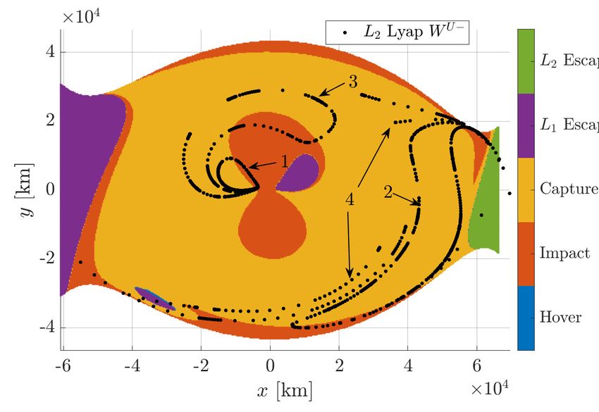
large energy changes. One strategy to accomplish a sizable energy change via low thrust is a low-
thrust spiral; 9 by combining spiraling motion with other structures, end-to-end transfers may be
designed. 10,11,12 This investigation supplies new insights to guide high-energy lunar capture by ap-
plying Poincaré mapping strategies. In particular, apses along low-thrust spiral trajectories near the
Moon are explored and linked to other ballistic and low-thrust paths to supply preliminary trajectory
designs and control histories.

BACKGROUND

  The first step in computing and leveraging dynamical structures within the CR3BP and the
CR3BP+LT is the development of the dynamical models. An energy-based approach is employed to
derive the governing equations in the CR3BP and produce an expression for the natural Hamiltonian.
By augmenting the CR3BP equations of motion (EOMs) with a low-thrust term, the CR3BP+LT is
constructed. Finally, invariant manifolds associated with periodic orbits and apse maps are intro-
duced as structures to be leveraged for this analysis.

Circular Restricted 3-Body Problem

   The CR3BP describes the motion of a relatively small body, such as a spacecraft, in the presence
of two larger gravitational point masses (P1 and P2 ) with paths that evolve along circular orbits
about their mutual barycenter (B). To simplify the governing equations and enable straightforward
visualization of periodic solutions, the motion of the spacecraft is described in a right-handed frame
(x̂, ŷ, ẑ) that rotates with the two primaries, as seen in Figure 1, where x̂, ŷ, and ẑ are vectors of
unit length. The system is parameterized by the mass ratio, µ = M2 /(M1 +M2 ), where M1 and M2

                                            ~
                                   ~ŷ      Ŷ

                                                    Spacecraft (x, y, z)

                                                            ~r23
                                                 ~r13                   ~x̂
                                                                   P2
                                                        θ                     ~
                                     P1                                       X̂
                                              B
                                Figure 1: CR3BP system configuration

are the masses of the primaries and M1 ≥ M2 . To facilitate numerical integration, the dimensional
values are nondimensionalized by characteristic quantities such that the distance between P1 and
P2 is unity, the mean motion of the two primaries is unity, and the masses of each body range from
zero to one. 13 The spacecraft is located relative to the system barycenter in the rotating frame via
the vector ~r = {x y z}T .
  The equations of motion governing the CR3BP are derived via a Hamiltonian energy approach.
Let the natural Hamiltonian be expressed as

                                  1      1 2     1−µ     µ
                            Hnat = v 2 −   x + y2 −     −     ,                                       (1)
                                  2      2          r13   r23

                                                        2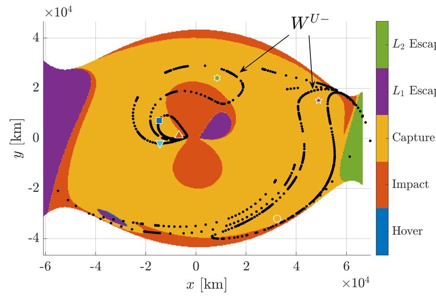
where r13 and r23 are the distances between the spacecraft (P3 ) and the two primaries,
                     p                                  p
              r13 = (x + µ)2 + y 2 + z 2 ,        r23 = (x − 1 + µ)2 + y 2 + z 2 ,
and v is the magnitude of the rotating velocity vector, v 2 = ẋ2 + ẏ 2 + ż 2 . By applying Hamilton’s
canonical equations of motion, a set of differential equations that govern the motion of P3 emerges,
                                           ẍ = 2ẏ + Ωx ,                                          (2)
                                           ÿ = −2ẋ + Ωy ,                                         (3)
                                           z̈ = Ωz ,                                                (4)
where Ω is the CR3BP pseudo-potential function,
                                     1              1−µ     µ
                                  Ω = (x2 + y 2 ) +      +     ,                                    (5)
                                     2               r13   r23
and Ωx , Ωy , and Ωz represent the partial derivative of Ω with respect to the subscripted state vari-
ables x, y, and z, respectively. Because the CR3BP is autonomous and conservative, Hnat is con-
stant and proportional to the Jacobi constant, C = −2Hnat , commonly leveraged as a measure of
the energy associated with arcs in the CR3BP.

CR3BP Incorporating Low-Thrust
  To incorporate low-thrust into the CR3BP, the low-thrust acceleration vector is first defined. This
vector,
                                          ~alt = alt û ,                                         (6)
is oriented relative to the rotating frame via the unit vector û and scaled by the nondimensional
acceleration magnitude, alt = f /m. In this expression, f represents the nondimensional thrust
magnitude and m is the nondimensional spacecraft mass, m = M3 /M3,0 , where M3 is the instanta-
neous spacecraft mass and M3,0 is the initial (wet) spacecraft mass. In the Earth-Moon CR3BP+LT,
f values on the order of 1e-2 are representative of current technological capabilities, as listed in
Table 1. When this additional acceleration is incorporated into the CR3BP dynamics, the equations

                            Table 1: Low-Thrust Spacecraft Parameters
                                       M3,0    F             alt   f (Earth-Moon)
                   Spacecraft
                                        kg     mN           m/s2       nondim

                   Deep Space 1 14     486     92.0    1.893e-4        6.95e-2
                   Hayabusa 15         510     24.0    4.706e-5        1.73e-2
                   Dawn 16             1218    92.7    7.611e-5        2.79e-2
                   Lunar IceCube 3      14     1.15    8.214e-5        3.01e-2

of motion become
                                       ẍ = 2ẏ + Ωx + alt ux ,                                     (7)
                                       ÿ = −2ẋ + Ωy + alt uy ,                                    (8)
                                       z̈ = Ωz + alt uz ,                                           (9)
                                             −f l∗
                                      ṁ =            ,                                            (10)
                                            Isp g0 t∗

                                                   3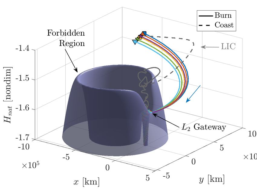
where ux , uy , and uz are the individual components of û along each of the rotating axes, l∗ and t∗
are the characteristic length and time quantities that nondimensionalize the CR3BP+LT coordinates,
Isp is the specific impulse associated with the propulsion system, and g0 = 9.80665e-3 km/s2 .
  In general, the natural Hamiltonian is not constant in the CR3BP+LT. The scalar time derivative,
Ḣnat , is related to the low-thrust acceleration via the relationship,

                                            Ḣnat = ~v • ~alt ,                                     (11)

where ~v is the spacecraft velocity as observed in the rotating frame. 17 This rate is extremized when
the two vectors are parallel, i.e., the natural Hamiltonian changes most rapidly when the thrust is
aligned with the velocity (or anti-velocity) vector. Because this “energy-optimal” control strategy
yields a non-autonomous system, few insights exist to guide design efforts for trajectories that em-
ploy such a technique. To mitigate a lack of understanding, this investigation explores the dynamics
of the CR3BP+LT with the energy-optimal thrust. The analyses are restricted to the planar dynamics
(z = ż = 0 ∀ t) to facilitate visualization and to clarify the complex dynamics.

Invariant Manifolds
   Although the CR3BP is largely characterized by chaotic motion, several useful structures, includ-
ing periodic orbits and the associated invariant manifolds, supply order and are frequently leveraged
in trajectory design applications. 18 In the planar problem, these manifolds act as separatrices and,
when combined with the forbidden regions, isolate trajectories that pass between the two primaries
from trajectories that remain bounded near one of the primaries (or that remain exterior to the system
as whole). 4

Apse Maps
   When the properties of periodic orbits and their manifolds are unavailable (either because they are
unknown, or because the system is non-autonomous), Poincaré maps may be        n employed to explore  o
the system. A map includes three key components: a set of initial conditions, ~qi,0 , i = 1, 2, . . . n ,
a hyperplane, Σ, and a visualization strategy. The initial conditions are numerically integrated to
the hyperplane for p returns, yielding the mapping, MpΣ (~qi,0 ). In many applications the hyperplane
is a geometric plane, e.g., a plane at some x, y, or z value, but Σ may also be a non-geometric plane.
For example, apse maps are employed in this investigation to visualize flow patterns near the Moon.
An apse is a point where the relative velocity between the spacecraft and a primary body is zero,
i.e., a point such that
                                     ṙk3 = (~r − ~rk ) • (~v − ~vk ) = 0,                           (12)
where ~rk and ~vk are the position and velocity of the k th primary body in the rotating frame. For lunar
capture applications, apses relative to P2 (i.e., the Moon in the Earth-Moon) system are of particular
interest; the initial states are selected near the Moon, where each initial state is a planar apse with
respect to the Moon at a specific Hnat value. Because these initial states all satisfy Equation (12)
and are all characterized by the same Hnat value, the four-dimensional planar problem is reduced
to two dimensions, enabling straightforward visualization of the complete dynamics (i.e., the full
4D state is recovered from a 2D representation). One common visualization strategy for apse maps
is to color the initial apse states by the behavior of the resulting arc, as illustrated in Figure 2. The
initial state for a trajectory that impacts the Moon (i.e., that reaches a position within the physical
lunar radius) at or prior to the p = 2 map returns is colored orange, while the initial states for

                                                    4
Figure 2: A ballistic lunar apse map at Hnat = −1.584 for p = 2 map returns in Moon-centered
rotating coordinates.
trajectories that depart through the L1 and L2 gateways are colored purple and green. Trajectories
that remain in the lunar region (r23 < 115, 500 km) are termed “captured,” and the associated
initial states are depicted in yellow. Clear structures, i.e., colored lobes, are visible in the map;
these structures can be linked to other known structures in the CR3BP. For example, the invariant
manifolds associated with the L1 and L2 Lyapunov orbits at the same Hnat value bound the L1 and
L2 escape regions. 19,20,21 Accordingly, an apse map with this visualization scheme supplies useful
information for capture applications. A spacecraft entering the lunar region may target an apse in
one of the capture regions to remain near the Moon for at least p map returns; if an apse along the
incoming trajectory is located in one of the escape regions, the spacecraft will depart within p map
returns.
LOW-THRUST APSE MAPS
Apse maps may also be employed in the CR3BP+LT with anti-velocity-pointing thrust to explore
options for lunar capture. The map is constructed in the same way as the ballistic map: a set of apses
near the Moon, all at a consistent Hnat value, are propagated for p returns to the apse hyperplane
and colored by the fate of the resulting trajectory. When the thrust magnitude is very small, as in
Figure 3(a), the low-thrust apse maps appear very similar to the ballistic maps. However, as the
thrust magnitude increases, the structures on the map change, as illustrated in Figure 3(b). For
example, the low-thrust apse map for f = 3e-2 (consistent with the capabilities of Lunar IceCube)
retains a teardrop-shaped lobe of L1 escape motion near the center of the map, as well as some L1
and L2 escape regions on the left and ride sides of the plot. However, there is significantly less
escape motion in the center of the plot; instead, many more options for capture exist. Because the
propagation is implemented with anti-velocity-pointing thrust, a strategy to decrease Hnat , it is not
surprising that fewer arcs escape during the two map returns. As the energy decreases, the L1 and
5(a) Lunar IceCube Capability: f = 3e-2 (b) Deep Space 1 Capability: f = 7e-2
Figure 3: Low-thrust lunar apse maps for Hnat = −1.584 and p = 2 in Moon-centered rotating
coordinates. The initial states are propagated with anti-velocity-pointing thrust with Isp = 2500
seconds.
L2 gateways close, prohibiting transit from the lunar region. At a larger thrust magnitude of f = 7e-
2 (a Deep Space 1 capability), the apse map, plotted in Figure 3(b) includes even more opportunities
for capture. While the boundaries of these regions are defined by the L1 and L2 Lyapunov manifolds
in the ballistic problem, no such structures are known to bound the regions on the low-thrust apse
maps. Because the thrust orientation, âlt , is aligned with the evolving anti-velocity vector, the
CR3BP+LT is nonautonomous, does not admit an integral of the motion, and includes no periodic
solutions. Accordingly, the low-thrust apse maps must be constructed by propagating each of the
initial conditions to determine its fate.
The low-thrust maps include a new type of behavior, colored blue and termed “hover” motion,
that is not present in the ballistic map. These initial states yield trajectories that, when propagated
with anti-velocity-pointing thrust, eventually reach a velocity magnitude of zero. Due to the imple-
mentation of the control law, as the velocity magnitude approaches zero (numerically equivalent to
2−52 nondimensional units, or about 2.27e-16 km/s in the Earth-Moon system), as in Figure 4(b),
the orientation of the velocity vector is poorly defined, oscillating with numerical noise as well
as the with spacecraft motion. Accordingly, the hover is accomplished by rapidly reorienting the
low-thrust acceleration vector, an impractical control method in practice.
Despite the practical difficulty of accomplishing a hover maneuver, the associated map regions
supply insights for trajectory design. In the maps depicted in Figure 3, the initial states that yield
hover motion are located on several of the boundaries between states linked to captured motion and
states associated with L1 or L2 escape. A sample of the trajectories initiated from these states,
plotted in Figure 4, illustrate the differences between the regions. The initial states for the five
sample arcs are selected in a horizontal line at y = 16, 384.6 km spanning the blue hover region
near x = 6 × 10⁴ km in Figure 3(b). (A similar band of hover motion is included in the map for
f = 3e-2 at the boundary between capture and L2 escape motion in the L2 gateway.) The arcs,
plotted in position space in Figure 4(a), initially flow along the −ŷ direction toward L2 and toward
a set of low-thrust equilibria, termed a zero acceleration contour (ZAC), plotted in gray. The ZAC
~ = ~0 with f = 7e-2, each point associated with a
is a set of points that satisfy the equation ∇Ω
17
unique orientation of û. One intuitive hypothesis to explain the hover motion is that the arcs reach
6(a) Moon-centered Earth-Moon rotating frame with (b) The hover arcs reach a velocity magnitude of
the low-thrust zero acceleration contours (ZACs) zero
for reference
Figure 4: Sample arcs from the low-thrust apse map in Figure 3(b); the “hover” arcs (blue) reach a
zero velocity magnitude in the vicinity of the ZAC
one of these equilibria states. However, because û changes continuously with the orientation of ~v
when the velocity-pointing control law is employed, no single point on the ZAC is associated with
a trajectory; during the hover maneuvers (located at the ends of the blue arcs), the location of the
instantaneous low-thrust equilibrium solution changes as rapidly as the orientation of û. Accord-
ingly, the hover arcs do not intersect an equilibrium point. In fact, the locations where the arcs reach
v = 0 are unrelated to the ZAC. Instead, the hover locations are the points where the forbidden re-
gions “catch up” with the low-thrust trajectory. Recall that Hnat decreases monotonically when the
anti-velocity-pointing control law is applied; thus, as the trajectories evolve from the initial states
on the apse map, the forbidden regions grow, increasingly restricting the motion of the spacecraft.
At the hover locations, the boundary of a forbidden region, a zero velocity contour, 13 intersects with
the trajectory, leaving the space “in front” of the hover location (i.e., in the direction of the trajec-
tory evolution prior to the hover) accessible but the area “behind” the hover location inaccessible.
Having reached a lower Hnat value, an alternative control technique (a velocity-aligned direction
is undefined) may be employed to further influence the trajectory evolution. Indeed, the low-thrust
acceleration is particularly influential on the spacecraft path due to the low velocity magnitude at
these points. Thus, the map states associated with hover motion are candidates for further study.
HIGH-ENERGY CAPTURE STRATEGIES
Two strategies to design high-energy, low-thrust lunar capture trajectories are explored. The first
scheme leverages a low-thrust apse map to identify points in the lunar region at a high Hnat value
that result in captured motion. The second technique augments an L2 Lyapunov manifold with
low-thrust to decrease the Hnat value along the trajectory before arriving in the lunar region, where
a similar (but lower energy) low-thrust apse map is employed to identify capture options. In both
strategies, the low-thrust force is aligned with the anti-velocity direction to supply the maximum
Hnat rate of change.
7Lunar IceCube
The Lunar IceCube trajectory is referenced as a source of realistic parameters to illustrate the
proposed design strategies. Lunar IceCube (LIC), a 14 kilogram, 6U “cubesat”, is equipped with
a low-thrust propulsion system that can deliver up to 1.15 millinewtons (f ≈ 3e-2 in the Earth-
Moon CR3BP+LT) of force with a specific impulse, or Isp , of 2500 seconds. 3 About 5 days after
deployment from EM-1, LIC flies past the Moon, as illustrated in Figure 5, and the subsequent
trajectory extends far from the Earth and Moon. A little less than six months later, the spacecraft
(a) Earth-Centered J2000 frame (b) Earth-Centered Earth-Moon rotating frame
(c) Earth-Centered Sun-Earth rotating frame (d) Earth-Centered Earth-Moon rotating frame
Figure 5: Planar projections of a LIC trajectory option in a variety of reference frames; blue arcs
represent ballistic (coasting) motion, while red arcs indicate that the low-thrust engine is active
(burning). This baseline solution begins at a deployment epoch of June 27, 2020 at 21:08:03 UTC,
and ends in a low-lunar orbit on May 22, 2021.
returns to the Moon and employs the low-thrust propulsion system to decrease the orbital energy
and capture into a polar lunar orbit. For the current analysis, only the final approach to the Moon
and the subsequent energy decrease and capture are considered. During this final phase, the Hnat
value in the Earth-Moon rotating frame remains between -1.53 and -1.4; the Hamiltonian fluctuates
because the trajectory is propagated in an ephemeris model in which Hnat is not an integral of the
motion. Accordingly, Hnat values in this range are employed as reasonable values to illustrate the
proposed capture strategies. Additionally, while the trajectory does include several small thrusting
8arcs prior to the long, final burn, the mass change is negligible (0.011 kg of the 14 kg wet mass),
thus, the initial mass for all capture strategies is set to 100%.
Capture Initiated Near the Moon
One strategy for high-energy capture initiates thrusting in the anti-velocity direction when the
spacecraft arrives in the vicinity of the Moon, as illustrated by the Lunar IceCube (LIC) trajectory
in Figure 5. Clearly, capture near the Moon is accomplished in this specific scenario, but the single
LIC trajectory does not supply information about other nearby solutions. For a more general view
of capture opportunities in the lunar region, an apse map is constructed. Consistent with the LIC
trajectory, the set of initial states is characterized by an Hnat value of -1.425, and the propagation
is modeled with an Isp value of 2500 seconds. Two thrust magnitudes are employed: the LIC thrust
capability of f = 3e-2, and a larger thrust magnitude of f = 7e-2, consistent with a Deep Space
1 capability. To explore capture options, each point on the map is propagated for up to 20 map
returns (i.e., apses), and the initial conditions are colored by the fate of the associated trajectory,
consistent with the scheme in Figure 2. The resulting maps, plotted in Figure 6, are dominated
by escaping trajectories. The lack of other types of motion is not surprising given the high energy
(a) Lunar IceCube Capability: f = 3e-2 (b) Deep Space 1 Capability: f = 7e-2
Figure 6: Apse maps in the Moon-centered Earth-Moon rotating frame for Hnat = −1.425, Isp =
2500 seconds, and p = 20 map returns.
and small thrust force; at energies this high, the low-thrust propulsion is generally not sufficient to
prevent the spacecraft from departing the lunar region. (For these high energy maps, departure is
defined by the radius r23 > 385, 000 km.) However, thin bands of more nuanced behavior appear
in the maps between the large regions of L1 and L2 escapes. Zooming in on the structures within
the black boxes in Figure 6, as depicted in Figure 7, reveals even thinner bands of initial conditions
with different fates. At the resolution available in these maps, no capture options are revealed for
the LIC thrust capability. This result does not necessarily preclude capture at this energy and thrust
capability; a modified thrust strategy may adjust some of the collision arcs to achieve capture. When
a larger thrust magnitude is employed, as in Figure 7(b), capture opportunities become available.
These apses, colored yellow on the map, correspond to arcs that pass through 20 apses without
9(a) Lunar IceCube Capability: f = 3e-2 (b) Deep Space 1 Capability: f = 7e-2
Figure 7: Close-up views of the apse map regions marked by black squares in Figure 6 reveal
chaotic motion; Moon-centered Earth-Moon rotating frame
colliding with the Moon or departing the lunar region. Although capture opportunities are apparent
at the higher thrust capability, they are generally isolated and located on the boundaries between
bands of other behaviors, in contrast with the dense bands of L1 escape, L2 escape, and impact
motion. Indeed, one of the defining characteristics of the high-energy apse maps in Figures 6 and 7
is chaos: initial states at apses located close together frequently yield very different arcs, particularly
in the thin bands viewed in Figure 7. Selecting several points in this regions with impact and
capture motion, as labeled in Figure 7, and plotting the associated trajectories, visualized in Figure
8, illustrates the chaotic nature of the dynamics. For each set of arcs, the initial conditions are
(a) Lunar IceCube Capability: f = 3e-2 (b) Deep Space 1 Capability: f = 7e-2
Figure 8: The arcs associated with the points labeled in Figure 7 illustrate the chaotic nature of the
dynamics; Moon-centered Earth-Moon rotating frame
located at a consistent y-coordinate, and are separated by an x distance of less than 39 kilometers
(the velocity magnitude is a function of the Hnat value and the velocity direction is orthogonal to
the ~r23 vector). Despite the similar initial states, the evolution of each trajectory varies significantly.
Although no capture opportunities are apparent for the LIC thrust magnitude of f = 3e-2, the
10geometries of the arcs represented by the map are similar to the LIC ephemeris solution. For ex-
ample, the large lobe common to the arcs in Figure 8(a) is very similar to the LIC trajectory at the
beginning of the thrust arc that delivers the spacecraft to lunar orbit, plotted in Figure 5(b). These
similarities, as well as first-hand knowledge of the difficulties associated with designing the LIC
trajectory, suggest that the chaos observed in the this planar apse map is consistent with the spatial
ephemeris model.
For either of the thrust levels, opportunities for capture exist only in the thin, chaotic bands.
Accordingly, a design strategy that initiates the capture burn near the Moon is likely to be sensitive,
diverging from the desired behavior when small perturbations are encountered. This sensitivity
affects not only the design process, but has implications for operations as well. Any failure in the
propulsion or navigation systems are likely to effect large changes on the trajectory and may place
the spacecraft on a path that does not capture near the Moon, effectively ending a cubesat mission
like Lunar IceCube or LunaH-Map.
Capture Initiated Far from the Moon
As an alternative to a strategy that initiates the capture sequence at a location near the Moon,
consider a strategy that employs low thrust to decrease the Hnat value prior to arrival at the Moon.
As illustrated in the apse maps for Hnat = −1.584, depicted in Figure 2, opportunities for capture
are more abundant and less chaotic at lower energies than the high-energy results illustrated in
Figure 6. In fact, a majority of the points on the low-energy map represent capture opportunities
with far less sensitivity than the options at Hnat = −1.425. Accordingly, a spacecraft that enters
the lunar region with an lower Hnat energy value is afforded more flexibility in achieving lunar
capture; even if the baseline trajectory is perturbed from a specific target, the spacecraft is unlikely
to rapidly depart the region.
To isolate low-thrust arcs that reach the lunar vicinity at a low energy, the invariant manifolds
associated with a ballistic L2 Lyapunov orbit are employed. In previous studies, such arrival arcs
have been produced by propagating a trajectory in reverse time from a low lunar orbit to some en-
ergetic or physical hyperplane. 3 While this method reveals capture paths, it restricts the exploration
to a specific destination orbit. By utilizing the separatrix property of the L2 Lyapunov manifolds, a
more general set of capture options may be constructed. The proposed capture strategy is comprised
of several steps:
1. Propagate the stable manifold, W S+ , associated with an Earth-Moon L2 Lyapunov orbit in
reverse time to a hyperplane, Σ1 , that is located exterior to the L2 gateway.
2. Propagate the stable manifold states with anti-velocity-pointing low-thrust in reverse time
from Σ1 to another hyperplane, Σ2 that serves as an interface between a high-energy trajectory
incoming to the Moon and a low-thrust arc that decreases the Hnat energy.
3. Construct a low-thrust apse map (anti-velocity-pointing thrust, forward time) at the same
Hnat energy value as the L2 Lyapunov orbit
4. Overlay the ballistic unstable manifold, W U − , associated with the L2 Lyapunov orbit on the
low-thrust apse map and identify intersections with capture opportunities.
From a mission sequence (i.e., forward time) perspective, a spacecraft approaching the Moon first
targets a state at Σ2 “inside” W̃lt . At Σ2 , the low-thrust propulsion is enabled with an anti-velocity-
11pointing orientation and the spacecraft proceeds to Σ1 . During this propagation, the Hnat value
along the trajectory decreases to match the energy associated with the L2 orbit. At Σ1 , the low-
thrust force is disabled and the trajectory is allowed to evolve ballistically, bounded by the L2
Lyapunov manifold separatrix, W S+ and then W U − . Apses on the trajectory during this ballistic
evolution are plotted on the apse map and compared with the low-thrust behavior available at each
apse; assuming one or more of the apses correspond to a low-thrust trajectory that captures about
the Moon, the low-thrust propulsion is re-enabled at the appropriate apse to begin a low-thrust spiral
into a low-energy lunar orbit.
To illustrate this sequence, parameters consistent with the LIC trajectory are again employed.
Select an L2 Lyapunov orbit with an Hnat value of -1.584, a low energy level that still permits transit
through the L2 gateway. The stable manifold that arrives at the orbit from the right side, W S+ , is
propagated in reverse time to the Σ1 hyperplane, located exterior to the system at x = 81, 422.6 km
in the Moon-centered Earth-Moon rotating frame, as depicted in Figure 9(a). At this hyperplane,
(a) The low-thrust arcs (red) flow directly into and (b) Initial conditions for the low-thrust arcs are se-
onto the ballistic L2 Lyapunov manifold (blue); lected at Σ1 from the interior (red points) of the bal-
Moon-centered Earth-Moon rotating frame. The listic manifold, and from the manifold itself (blue);
ballistic motion is bounded by the forbidden region tube topology at x = 81, 422.6 km
at Hnat = −1.584
Figure 9: At the Σ1 hyperplane, low-thrust arcs flow into and onto the ballistic L2 Lyapunov
manifold
a tube-topology representation of the manifold is constructed, 22 consisting of a radial coordinate,
r = (y− ỹ)/(2ỹ), and an angular coordinate θv = arctan(ẏ/ẋ). For this application, ỹ is selected to
be the y-coordinate of the nearest upper (y < 0) edge of the forbidden region. When plotted in polar
form, as in Figure 9(b), this topology supplies a full representation of the planar states (i.e., all four
Cartesian components of the state vector are available from the 2D representation). Because the full
state is represented on the map, determining whether a planar trajectory exists within the manifold
separatrix is straightforward - simply consider if the trajectory is encircled by the manifold contour
on the map. Leveraging this technique, a set of states inside the manifold are selected (plotted as
red dots in Figure 9(b)). These states are then employed as initial conditions for low-thrust arcs
that are propagated in reverse time with anti-velocity-pointing thrust to the second hyperplane, Σ2 .
Additionally, the manifold states (plotted in blue) are also propagated to Σ2 with the same thrust
strategy, yielding the W̃lt set; although these arcs appear similar to a manifold structure, they are
12not mathematically related to the originating periodic orbit, nor are they manifold arcs associated
with a low-thrust periodic orbit. 17
The Σ2 hyperplane serves as an interface between an incoming high-energy trajectory and a
low-thrust arc that decreases the Hnat energy. To facilitate high-energy capture, Σ2 should be
sufficiently far from the low-energy W S+ manifold such that the energy change along the low-
thrust arcs between Σ2 and Σ1 is large. Placing the Σ2 hyperplane at x = −687, 871.5 km (again
in the Moon-centered Earth-Moon rotating frame), as illustrated in Figure 10(a), supplies an energy
change consistent with the LIC trajectory. At this interface, a mapping strategy similar to the tube
(a) The low-thrust arcs (red) originate at the Σ2 hy- (b) A projection of the low-thrust states at Σ2 .
perplane, and have a similar geometry to the Lu- Low-thrust arcs propagated from the stable man-
nar IceCube (LIC) approach path; Moon-centered ifold (black) completely enclose low-thrust arcs
Earth-Moon rotating frame propagated from the interior of the manifold
Figure 10: Low-thrust trajectories that flow into a ballistic manifold decrease the Hnat value while
simultaneously delivering the spacecraft to the lunar vicinity; Moon-centered Earth-Moon rotating
frame
topology employed at Σ1 is applied; the y-coordinate of the arcs replaces the scaled y-coordinate,
but the velocity angle, θv , is identical to the previous definition. However, in contrast to the map
at Σ1 , this mapping cannot represent the full state in a 2-dimensional plot due to the variations in
the Hnat values associated with the low-thrust arcs at Σ2 . Accordingly, Hnat is included in the
mapping, yielding a 3-dimensional surface, a projection of which appears in Figure 10(b). This
mapping illustrates a similar structure: The low-thrust arcs propagated from within the ballistic
manifold, plotted in red, remain within low-thrust arcs propagated from the manifold itself, W̃lt ,
plotted in black. In contrast to the ballistic CR3BP, this apparent low-thrust separatrix behavior
is not predicted by the dynamics, but it does persist across a variety of Σ2 locations and a variety
of Hnat energy values. Increasing the density of the low-thrust arcs propagated from within the
ballistic manifold confirms this separatrix behavior: all of the points within W̃lt flow into W S+ .
While this analysis is conducted in the Earth-Moon CR3BP+LT, solar gravity is a non-negligible
force far from the system barycenter, i.e., along the arcs that approach Σ2 . The geometry of the LIC
trajectory, propagated in an Earth-Moon-Sun ephemeris model, is different than the Earth-Moon
arcs despite the similarities in the states at Σ2 , as illustrated in Figure 10(b). Indeed, previous in-
vestigations note the importance of solar gravity during this approach to the Earth-Moon system. 3
However, including the Sun in the model eliminates the autonomous nature of the gravitational dy-
13namics, complicating the analysis by adding an epoch-dependency. Thus, to develop the proposed
capture strategy, solar gravity is omitted from the model. For mission-specific applications, a rel-
evant epoch (or range of epochs) limits the scope of the design problem, and the low-thrust arcs
may be propagated between Σ1 and Σ2 in the appropriate dynamical environment. Regardless of
the specific model employed for the approach to Σ1 , the method remains unchanged.
Once a spacecraft has navigated through the low-thrust “tube”, W̃lt , and, subsequently, the bal-
listic W S+ manifold, the trajectory remains bounded by the L2 Lyapunov unstable manifold that
departs the orbit to the left, W U − . However, the Hnat energy associated with the trajectory and
the bounding manifold are not sufficiently low to prevent escape from the lunar region. Accord-
ingly, additional thrusting must be incorporated to reduce the Hnat value, i.e., to capture about the
Moon. The low-thrust apse map constructed at the same energy level as the ballistic manifold with
anti-velocity-pointing thrust, plotted in Figure 11, identifies locations in the lunar region where the
thruster may be re-activated to capture in a low-energy orbit about the Moon. Note that this map is
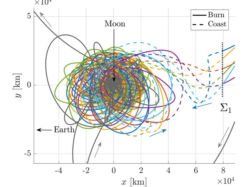
Figure 11: Ballistic L2 Lyapunov unstable manifolds (black) overlaid on a low-thrust apse map
(anti-velocity-pointing, f = 3e-2, Isp = 2500 sec) for Hnat = −1.584 and p = 20; Moon-centered
Earth-Moon rotating frame
constructed with the same parameters as the map in Figure 3(a), but this latter map is propagated
to 20 apses (a sufficient amount of time for the low-thrust force to decrease the Hnat value such
that both gateways are closed) whereas the map in Figure 3(a) is propagated to only two apses.
Accordingly, the 20-return map includes all of the information available in the 2-return map; every
escape and impact condition from the 2-return map is captured by the 20-return map. However,
some of the initial conditions that yield capture motion for two map returns escape or impact the
Moon when propagated for 20 returns. Overlaying the W U − ballistic manifold apses on the map
(plotted as black dots and labeled with map return number), reveals a specific subset of the capture
opportunities that are accessible from within the manifold separatrix. The first and second manifold
apse regions overlap almost entirely with capture opportunities; thus, nearly every arc within the
L2 Lyapunov manifold can be linked to a low-thrust path that delivers a capture trajectory. Con-
sequently, the majority of the arcs within W̃lt at Σ2 (Figure 10(b)) may be linked to a low-energy
lunar orbit.
14Several sample arcs are constructed to illustrate the capture process. The initial states for the
arcs are located within the W̃lt contour at Σ2 , as depicted by the colored symbols in Figure 12(a).
Each arc is propagated with anti-velocity-pointing low-thrust to Σ1 , where the thrust is disabled and
(a) Initial states for the arcs at Σ2 within the W̃lt (b) Intermediate states for the arcs at Σ1
contour
(c) Following a ballistic coast within W U − , each arc re-enables the
low-thrust force at an apse to capture about the Moon; Moon-centered
Earth-Moon rotating frame
Figure 12: Arcs that reach a low-energy lunar orbit are designed by identifying appropriate states
on the Σ2 , Σ1 , and apse maps
the arcs are allowed to evolve ballistically. The arcs coast for different time intervals: arcs 1 and
2 coast to the first apse, arcs 3 and 4 coast to the second apse, and arcs 5 and 6 coast to the third
apse. As expected, these apses, plotted as colored symbols in Figure 12(c), remain within the W U −
separatrix. Additionally, each of these apses is located in the yellow-colored capture region on the
low-thrust apse map. In contrast to the capture initiated near the Moon, the coast periods between
Σ1 and the subsequent apses provide opportunities for orbit determination and navigation updates
before the second low-thrust maneuver is initiated to capture near the Moon. Additional coasting
15time can be incorporated into the trajectory by directly targeting insertion onto the L2 Lyapunov
orbit, i.e., by following an arc on W̃lt and, equivalently, on W S+ , as illustrated by arc 1 in Figures
12(a) and 12(b). The initial state for arc 1, represented by a blue square, is located very near the
W̃lt boundary at Σ2 and remains near the W S+ contour at Σ1 . From the Σ1 hyperplane, a ballistic
coast along W S+ delivers the spacecraft to the Lyapunov orbit where an arbitrarily long coast may
be included. At some later time (e.g., when a phasing constraint is satisfied), a small maneuver is
sufficient to perturb the spacecraft from the periodic orbit and place it on the unstable manifold,
W U + , such that the spacecraft reaches the apses in Figure 12(c).
Although the six sample arcs are clearly separated on the Σ2 , Σ1 , and apse maps, the arcs follow
similar paths through configuration space. The physical trajectories, plotted in Figure 13, are par-
ticularly dense as the arcs approach the Moon. The Lunar IceCube (LIC) trajectory, plotted in gray,
(a) Configuration space representation in the (b) A zoomed view of the lunar region
Moon-centered Earth-Moon rotating frame
Figure 13: Sample capture trajectories in configuration space; Moon-centered Earth-Moon rotating
frame
follows a similar path as the the sample arcs, but differs considerably near the Moon. Although
many of these differences are a result of the different models employed to propagate the arcs (recall
that the LIC trajectory is propagated in a full, spatial ephemeris model whereas the sample arcs
are propagated in the planar, Earth-Moon CR3BP+LT), some of the differences are certainly due
to the thrust strategy. The sample arcs employ low-thrust to decrease the Hnat value, constraining
the approach geometry to flow through the L2 gateway. In contrast to these sample arcs, the LIC
trajectory, characterized by a much higher Hnat value and an initial ballistic coast, is not similarly
constrained.
Another useful illustration of the capture trajectories is the Hnat energy evolution through time
and space. The LIC trajectory, plotted in gray in Figure 14, coasts to the lunar vicinity before
initiating a low-thrust maneuver to decrease energy and capture near the Moon. (Because the LIC
trajectory is propagated in an ephemeris model with forces not included in the CR3BP+LT, such as
solar gravity, the Hnat value is not constant during the coast.) In contrast, the capture arcs designed
via the strategy detailed in this investigation initiate a low-thrust maneuver to decrease the Hnat
value immediately, as is evident in the time-history plotted in Figure 14(a). A spatial representation
of these planar trajectories in Figure 14(b) further illustrates the relationship between the Hnat value
16(a) Temporal representation (b) Spatial representation
Figure 14: The Hnat energy along the sample arcs and the LIC trajectory decreases to a low-energy
lunar orbit
along the arcs and geometry of the forbidden region. In this representation, each horizontal “slice”
of the forbidden region surface is the zero velocity contour at the corresponding Hnat value. The
planar projection of the LIC trajectory maintains a high Hnat value, remaining unconstrained by
the forbidden region. Rather than offering flexibility, this lack of an energy constraint results in
sensitivities that create design difficulties, as illustrated in the chaotic apse maps depicted in Figures
6 and 7. In contrast, the colored trajectories that employ thrusting to reduce the Hnat energy before
arriving at the Moon pass just above the L2 gateway and are relatively bounded near the Moon. As
a result, the ballistic coast arcs that begin at Σ1 remain captured for several returns to the apse map,
bounded by W U − . Thrusting may resume at any of the apses that overlap with low-thrust capture
motion to further decrease the Hnat value along the trajectory such that escape from the lunar region
is not possible, i.e., delivering the spacecraft to a low-energy lunar orbit.
CONCLUDING REMARKS
Trajectory designs that reduce the Hnat energy prior to arriving near the Moon benefit from re-
duced chaos compared to trajectories that begin energy-reducing maneuvers near the Moon. These
differences between the high-energy, high-chaos dynamics and the low-energy, low-chaos dynam-
ics are apparent when comparing energy-optimal low-thrust spirals on apse maps. Additionally, a
trajectory that reaches the lunar vicinity with a relatively low Hnat energy may incorporate coasting
segments prior to the final low-thrust maneuver, facilitating orbit determination and navigation up-
dates. While this analysis has focused on the lunar region, the capture strategies may be generalized
for capture about any secondary body in a CR3BP system. Additionally, capture via the L1 gateway
may be accomplished via similar processes. Finally, this investigation considers only the planar dy-
namics but may be applicable to the spatial realm. The separatrix properties of spatial manifolds are
less well-established than the separatrix nature of planar manifolds, but appear to behave similarly.
ACKNOWLEDGMENTS
This work was completed at Purdue University and at the Goddard Space Flight Center in Green-
belt, Maryland. The authors wish to thank the Purdue University School of Aeronautics and As-
17tronautics as well as the NASA Goddard Navigation and Mission Design branch for their facilities
and support. Additionally, many thanks to the Purdue Multi-Body Dynamics Research Group for
interesting discussions and ideas, with special thanks to Kenza Boudad and Robert Pritchett. This
research is supported by a National Aeronautics and Space Administration (NASA) Space Technol-
ogy Research Fellowship, NASA Grant NNX16AM40H.
REFERENCES
[1] M. L. McGuire, L. M. Burke, S. L. McCarty, K. J. Hack, R. J. Whitley, D. C. Davis, and
C. Ocampo, “Low-Thrust Cis-Lunar Transfers Using a 40 kW-Class Solar Electric Propulsion
Spacecraft,” AAS/AIAA Astrodynamics Specialist Conference, Columbia River Gorge, Steven-
son, Washington, Aug. 2017.
[2] C. Hardgrove, J. Bell, J. Thangavelautham, A. Klesh, R. Starr, T. Colaprete, M. Robinson,
D. Drake, E. Johnson, and J. Christian, “The Lunar Polar Hydrogen Mapper (LunaH-Map)
mission: Mapping hydrogen distributions in permanently shadowed regions of the Moon’s
south pole,” Annual Meeting of the Lunar Exploration Analysis Group, Vol. 1863, Columbia,
Maryland, Oct. 2015, p. 2035.
[3] N. Bosanac, A. D. Cox, K. C. Howell, and D. C. Folta, “Trajectory Design for a Cislunar
CubeSat Leveraging Dynamical Systems Techniques: The Lunar IceCube Mission,” Acta As-
tronaut., Vol. 144, Mar. 2018, pp. 283–296.
[4] C. Conley, “Low Energy Transit Orbits in the Restricted Three-Body Problem,” SIAM Rev.
Soc. ind. Appl. Math, Vol. 16, 1968, pp. 732–746.
[5] W. S. Koon, M. W. Lo, J. E. Marsden, and S. D. Ross, “Low Energy Transfer to the Moon,”
Celest. Mech. Dyn. Astron., Vol. 81, 2001, pp. 63–73.
[6] G. Gómez, W. Koon, M. Lo, J. Marsden, J. Masdemont, and S. Ross, “Connecting orbits and
invariant manifolds in the spatial restricted three-body problem,” Nonlinearity, Vol. 17, No. 5,
2004, pp. 1571–1606.
[7] G. Mingotti, F. Topputo, and F. Bernelli-Zazzera, “Low-Energy, Low-Thrust Transfers to the
Moon,” Celest. Mech. Dyn. Astron., Vol. 105, 2009, pp. 61–74.
[8] R. Anderson and M. Lo, “Role of Invariant Manifolds in Low-Thrust Trajectory Design,” J.
Guid. Control Dyn., Vol. 32, Nov. 2009, pp. 1921–1930.
[9] A. Petropoulous and J. Sims, “A Review of Some Exact Solutions to the Planar Equations of
Motion of a Thrusting Spacecraft,” 2nd International Symposium on Low Thrust Trajectories,
Toulouse, France, June 2002.
[10] D. Grebow, M. Ozimek, and K. Howell, “Design of Optimal Low-Thrust Lunar Pole-Sitter
Missions,” J. Astronaut. Sci., Vol. 58, Jan. 2011, pp. 55–79.
[11] A. Moore, S. Ober-Blöbaum, and J. Marsden, “Trajectory Design Combining Invariant Man-
ifolds with Discrete Mechanics and Optimal Control,” J. Guid. Control Dyn., Vol. 35, Sept.
2012, pp. 1507–1525.
[12] A. Das and K. Howell, “Solar Sail Transfers from Earth to the Lunar Vicinity in the Circular
Restricted Problem,” AAS/AIAA Astrodynamics Specialist Conference, Vail, Colorado, Aug.
2015.
[13] V. Szebehely, Theory of Orbits: The Restricted Problem of Three Bodies. New York: Aca-
demic Press, 1967.
[14] M. Rayman, P. Varghese, D. Lehman, and L. Livesay, “Results From the Deep Space 1 Tech-
nology Validation Mission,” International Astronautical Congress, Session IAA.11.2: Small
Planetary Missions, Amsterdam, The Netherlands, 1999.
18[15] H. Kuninaka, K. Nishiyama, Y. Shimizu, I. Funaki, and H. Koixumi, “Hayabusa Asteroid
Explorer Powered by Ion Engines on the way to Earth,” 31st International Electric Propulsion
Conference, University of Michigan, Ann Arbor, Michigan, Sept. 2009.
[16] C. Russel and C. Raymond, The Dawn Mission to Minor Planets 4 Vesta and 1 Ceres. Berlin:
Springer, 2012.
[17] A. D. Cox, K. C. Howell, and D. C. Folta, “Dynamical Structures in a Low-Thrust, Multi-
Body Model with Applications to Trajectory Design,” Celest. Mech. Dyn. Astron., Vol. 131,
No. 12, 2019. Available Online.
[18] W. S. Koon, M. W. Lo, J. E. Marsden, and S. D. Ross, Dynamical Systems, the Three-Body
Problem and Space Mission Design. New York: Springer, 2011.
[19] M. E. Paskowitz and D. J. Scheeres, “Robust capture and transfer trajectories for planetary
satellite orbiters,” J. Guid. Control Dyn., Vol. 29, No. 2, 2006, pp. 342–353.
[20] D. C. Davis and K. C. Howell, “Characterization of trajectories near the smaller primary in the
restricted problem for applications,” J. Guid. Control Dyn., Vol. 35, Jan. 2012, pp. 116–128.
[21] K. Howell, D. Davis, and A. Haapala, “Application of Periapse Maps for the Design of
Trajectories Near the Smaller Primary in Multi-Body Regimes,” Mathematical Probl. Eng.,
Vol. 2012, 2012, pp. 1–22.
[22] T. Swenson, M. W. Lo, B. Anderson, and T. Gordordo, “The Topology of Transport Through
Planar Lyapunov Orbits,” AIAA SciTech Forum, Kissimmee, Florida, Jan. 2018.
19You can also read