Potential for Optimization in European Power Plant Fleet Operation - MDPI
←
→
Page content transcription
If your browser does not render page correctly, please read the page content below
Article
Potential for Optimization in European Power Plant
Fleet Operation
Bernhard-Johannes Jesse *          ID
                                        , Simon Morgenthaler   ID
                                                                    , Bastian Gillessen   ID
                                                                                               , Simon Burges and
Wilhelm Kuckshinrichs ID
 Forschungszentrum Jülich, Institute of Energy and Climate Research—Systems Analysis and Technology
 Evaluation (IEK-STE), D-52425 Jülich, Germany; s.morgenthaler@fz-juelich.de (S.M.);
 ba.gillessen@fz-juelich.de (B.G.); s.burges@fz-juelich.de (S.B.); w.kuckshinrichs@fz-juelich.de (W.K.)
 * Correspondence: b.jesse@fz-juelich.de; Tel.: +49-2461-61-3587

 Received: 20 November 2019; Accepted: 3 February 2020; Published: 7 February 2020

 Abstract: Energy policy makers need information about the greenhouse gas reduction potential
 that could be realized by changes to the operation of the currently existing European power
 plant fleet to enable short-term actions. Possible measures could reduce the climate impact of
 the European electricity system and, additionally, be realized quickly as new investments are avoided.
 In this paper, the Calliope based energy system model Stella of the European electricity system is
 presented and used for the first time, with the goal to quantify cost and CO2 emissions optimal
 operation strategies of the existing European power plant fleet. By applying the model to six scenarios
 the results show that the greenhouse gas emissions of the European power plant fleet could be reduced
 by more than 50% with little additional costs compared to today’s power generation mix. It is shown
 that historic power plant operation follows only economic considerations while not fully covering its
 climate impact. The results demonstrate to policy makers the scale of reduction potential that could
 be achieved by short-term actions.

 Keywords: greenhouse gas reduction; European power plant fleet; European electricity system;
 Calliope; Stella; energy system planning; emissions; power supply

1. Introduction
     Identification and evaluation of climate change mitigation strategies is a key objective of energy
systems analysis. As climate change progresses [1] and the pressure on energy policy makers to
act rises, more and more resources are directed into the development and usage of corresponding
energy system models in particular and the field of systems analysis in general [2]. Energy system
models are applied to answer research questions that are not limited to the resilience of energy
systems [3], the impact of changing heating and cooling demand due to climate change [4] or the
altering potentials of electricity generation by renewable energies [5]. The following studies show
applications of large-scale multi-regional energy system models in context of climate change mitigation
strategies: Löffler et al. [6] use the global energy system model GENeSYS to model scenarios with
special focus on coupling of electricity, transportation and heating sectors with a time frame up to the
year 2050. The authors suggest a photovoltaic dominated renewable energy mix to achieve agreed
global greenhouse gas reduction targets. Pursiheimo et al. [7] show similar results but further state the
importance of power-to-x technologies in a future global energy system. Additionally, Fattori et al. [8]
present an open local multi-regional energy system model in order to include citizens into the process
of energy system planning. The purpose is to establish a crowd-source development. Examples for
national energy system models and their usage in the context of climate change mitigation strategies
are Tahir et al. [9] for China or Heinrichs et al. [10] for Germany.

Energies 2020, 13, 718; doi:10.3390/en13030718                                       www.mdpi.com/journal/energies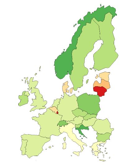
Energies 2020, 13, 718                                                                             2 of 22

      For reasons of quality, transparency, repetition and credibility, relevant energy system models
are more and more modeled in open source modeling frameworks like Calliope [11], FINE [12],
OSeMOSYS [13], PyPSA [14] or oemof [15]. The user models energy systems by paramerization and
combination of predefined items. Model results are typically calculated by mathematical programming
methods like continuous linear programming. An important issue is the establishment of required
open databases. The openmod-initiative motivates modelers to create and provide such data [16].
      Even though models and studies with focus on an optimal energy system design for future
challenges exist, a study on the amount of carbon dioxide (CO2 ) that could be saved within the
existing energy system design by changing its operation is missing. Therefore, the goal of this study
is the first quantitative estimation and discussion of a cost and CO2 emission optimal operation
strategy of the existing European power plant fleet. As changes in operation strategy do not cause
investments, improvements can be realized without significant cost increases. Therefore the energy
system model Stella is used to analyze the cause–effect relationships between cost and emission optimal
systems as well as model results and reality. Corresponding research questions are: What is the cost
optimal operation strategy for the European power plant fleet neglecting existing market mechanisms
e.g., ancillary services? What is the emission optimal strategy? How much CO2 emissions could be
avoided and what are the corresponding costs? Which obstacles should be considered? This work is
a debate contribution on how to mitigate climate change. An additional novelty of this work is the first
application of the open-source modeling framework Calliope for modeling the European electricity
system [11].
      In literature adjacent studies have been published. Nevertheless, none answer the above
mentioned research questions. Brown et al. [17] use a spatially and temporally resolved
sector-coupled model of Europe (PyPSA-EUR-SEC-30) to assess the impact of either expanded
cross-border transmission capacities or sector coupling in a 95% carbon dioxide reduction
scenario. Gerbaulet et al. [18] develop decarbonization scenarios of the European electricity sector.
Schlachtberger et al. [19] develop cost optimal scenarios of the European electricity system with special
respect to weather data, cost parameters and policy constraints. A main result is that a 57% CO2
reduction compared to the base year 1990 is also cost optimal.
      In order to firstly examine the CO2 and cost reduction potential of the existing European power
plant fleet by changing its operation strategy, the study is structured in the following way: The used
energy system model together with its data is presented in Section 2. The considered scenarios are
described in Section 3. Then, in Section 4, the results of the model runs are analyzed, and discussed in
Section 5, followed by the conclusion in Section 6.

2. Methodology
     In this work the optimizing energy system model Stella is used to analyze the effects of different
objective functions and constraints. The model created is based on Calliope [11]. The model was
created using Calliope version 0.6.3 and solved using Gurobi version 8.1.1. Calliope is a Python based
open source model framework. It is designed to model complex energy systems with a relatively
simple configuration and setup. The user may decide between continuous and mixed integer linear
programming. The mathematical formulation of all model equations and their implementation are
described in detail in the documentation of Calliope, which can be found on www.callio.pe [20].
     The model itself is a simplified representation of the European electricity system. It consists of
29 core regions and 11 outer regions. The core regions are the countries of the European Union as
well as Norway and Switzerland excluding Malta and Cyprus. In addition, Denmark is divided into
an eastern and a western region as they belong to different asynchronous control zones. Each of the
core regions is represented by a node, has country-specific access to technologies and a country-specific
demand for electricity. The outer regions consist of the following countries: Albania, Bosnia and
Herzegovina, Cyprus, Montenegro, North Macedonia, Northern Ireland, Serbia, Ukraine as well
as Morocco and Russia. These regions only have one technology available that acts as a source for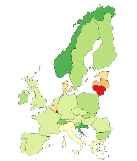
Energies 2020, 13, 718                                                                                  3 of 22

electricity. They are represented as one node each. The individual nodes of the entire model are
interconnected. For the net transfer capacities, values are interpolated from the 2010 statistical data [21]
and the planned 2020 values from the TEN-YEAR NETWORK DEVELOPMENT PLAN 2016 [22].
The net transfer capacities describe the net capacity to transmit electricity between two regions in the
model Figure 1 shows the regions covered in the model.

             @EuroGeographics

               Figure 1. Map of the modeled regions, core (light blue) and outer (deep blue) regions.

      On the map the core regions are coloured light blue whereas the outer regions are coloured deep
blue. Countries not modeled are shown in grey.
      In terms of technologies, a distinction is made between supply technologies and conversion
technologies. Conversion technologies produce electricity by consuming a fuel. Supply technologies
are sources for fuels, i.e., biomass, hard coal, lignite, natural gas, oil, uranium. For the outer regions
no further technology distinction is applied however outer regions can supply electricity to the core
regions for a fixed price. In the case of the power-generating conversion technologies, a distinction
can be made between ten different fuel groups. The fuel groups and their respective technologies are
listed in Table 1.

                                Table 1. Overview of fuel groups and technologies.

                                Fuel Group                Technologies
                                  Solar       Photovoltaic system
                                  Wind        Wind onshore, Wind offshore
                                   Oil        Steam turbine
                                   Gas        Open cycle gas turbine, Steam turbine,
                                              Combined cycle gas turbines
                                Hard coal     Steam turbine
                                 Lignite      Steam turbine
                                Nuclear       Steam turbine
                                Biomass       Steam turbine
                                 Hydro        Run-of-River, Reservoir storage
                                 Other        Waste, Geothermal system, Other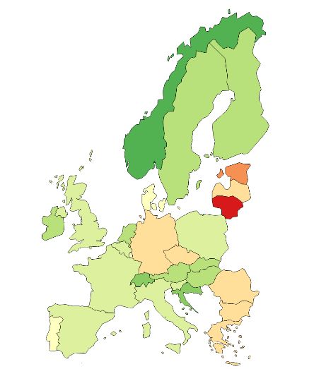
Energies 2020, 13, 718                                                                                4 of 22

      A future expansion of the model to cover other sectors and energy carriers is easily feasible.
Thus combined heat power plants are included as well as power-only plants. Even though the
focus is on the electricity sector heat generation from combined heat and power plants is tracked.
The model calculates both total system costs and total CO2 emissions. The model data are based on
the data from [23]. Installed power plant capacities are generated using the powerplantmatching
tool [24] that combines different power plant databases. The weather data used for photovoltaic and
wind turbines are from www.renewables.ninja [25,26], which provides bias corrected capacity factors.
The CO2 emissions for the technologies in the model are mostly based on [27]. The electricity demand
for the modelled regions are a model input and based on [28].
      The group-share constraint of Calliope is applied to configure the power generation of specific
fuel groups in individual countries in the model. This allows to set country-wise and fuel group-wise
relative share of produced electricity. Using this constraint, the model can be adjusted in such a way that
annual historical data is reproduced. However, this only applies with some limitations. For example,
the hourly power plant deployment does not match historical data. In addition, not all fuel groups
can be set in all countries, as otherwise the model will not compensate for statistical inconsistencies.
      Both input and output data of the model have an hourly resolution, which allows a detailed
analysis by time. In addition, the challenges arising from the fluctuation of wind and solar are better
represented than with a coarser temporal resolution. Moreover, storage effects and effects on different
time scales can be analyzed. An analysis of temporal resolution in energy system models and time
series aggregation methods that could be applied in case of computational congestions are given
in [29].
      All model runs conducted for this paper were carried out on a workstation, with following
specification: 16 CPU-Cores and 32 threads (Intel R Xeon R CPU E5-2667 v3 @ 3.2 GHz), 256 GB RAM
(DDR4 @ 2113 MHz), Windows 8.1 Pro 64-bit.

3. Scenarios
     For this analysis a total of six scenarios are developed to test the model and evaluate the ecological
and economic potential of the current European power plant fleet. They include different optimization
objectives and constraints. The optimization objectives are either minimizing the total system cost (all
scenarios starting with Mon for monetary) or minimizing total CO2 emissions (all scenarios starting
with Emi for emissions). The total system costs consist of the annualized investment, fixed operating
costs and fuel costs. For both objectives constraints are introduced step wise. However, electricity
demands and net transfer capacities for electricity are constant for all scenarios. In the Flex scenarios
the composition of installed capacity is a model result and is left completely free. In contrast, in the
Cap and CapShare scenarios, the capacities are model input. For the Cap scenarios the composition of
the installed capacities are fixed to the statistical data of the existing European power plant fleet from
2015 (cf. Section 2). In these cases the composition of the installed capacities is no longer a model result
but a model input. Thus, results show how the existing European power plant fleet can be operated in
a cost-optimal or an emission-optimal manner to meet the power demand. Finally, the composition of
the electricity production is fixed to the statistical data from 2015 in the CapShare scenarios. Due to
data inconsistency a few constraints for the fixed production share had to be relaxed for the CapShare
scenarios. Here, the model results will approximate the real total system costs and emissions as best as
model inputs and constraints allow. Table 2 gives an overview of the modelled scenarios.
Energies 2020, 13, 718 5 of 22
Table 2. Overview of scenarios.
Name Objective Capacity Fixed Production Share
Flex variable no
Mon Cap Total system costs 1 fixed hydro and other only
CapShare 2015 yes
Flex variable no
Emi Cap CO2 emission fixed hydro and other only
CapShare 2015 yes
Note: 1 As all capacities are an exogenous model input for the Cap scenarios the overall investments cost are fixed
and thus have no impact on the optimization process.
The CapShare scenarios are intended to validate the model and serve as a references for the
other scenarios. The MonCap and EmiCap scenarios are used to evaluate, respectively, the economic
and the ecological potential of the existing European power plant fleet. The Flex scenarios are
best-case scenarios.
4. Results
The model results are analyzed by a set of performance indicators comprising installed capacities,
load factors, total system costs and emissions as well as the share of electricity produced by the fuel
group. To validate the model, the results of the CapShare scenarios are compared with historical
data from [30]. This data stem officially from ENTSO-E, the European Network of Transmission System
Operators, which is the best source available for such data. Figure 2 shows the deviation of the load
factors of the fuel groups in the different regions.
0.004
0.002
Load factor
0.000
0.002
0.004
MonCapShare EmiCapShare
Figure 2. Deviation between CapShare scenarios and real world data for the load factor.
The representation as a box plot allows the statistical distribution of the deviation to be examined.
The deviation of the load factors are between 0.002 and 0.0 for the two scenarios. Outliers are not
shown but can be found in Appendix A (Figure A1). In addition to the validation with the load factors,
the generated electricity was also used for validation. Again, most deviations are in a very small
range. The corresponding figures can be found in Appendix A (Figures A2 and A3). The reason for
the discrepancy is twofold. Firstly, data inconsistencies in the statistical data. Secondly, the model
optimizes operation on the basis of annualized total system costs, whereas power plant operators often
decide operation based on marginal costs. However, in total, the deviations for both parameters are
very small. As the deviations for both scenarios are very small they can serve as a reference.Energies 2020, 13, 718 6 of 22
The time resolution chosen allows a detailed analysis of the calculated electricity production.
Figure 3a shows the temporal profile of electricity production over all core regions for the MonCapShare
scenario. A partial section for the week from 01 June 2015 to 07 June 2015 is given in Figure 3b to
enable a more detailed look.
500
Electricity generation [GW]
400
300
200
100
0
05
06
06
06
07
07
08
-0
-0
-0
-0
-1
-1
-1
6-1
7-1
8-1
9-1
0-1
1-1
2-1
5
5
5
5
5
5
5
Solar Oil Hard Coal Nuclear Hydro
Wind Gas Lignite Biomass Other
(a) European electricity generation by fuel group in 2015 (MonCapShare)
400
350
Electricity generation [GW]
300
250
200
150
100
50
0
01
02
03
04
05
06
07
-06
-06
-06
-06
-06
-06
-06
-15
-15
-15
-15
-15
-15
-15
Solar Oil Hard Coal Nuclear Hydro
Wind Gas Lignite Biomass Other
(b) European electricity generation by fuel group in the first week of June in 2015 (MonCapShare).
Figure 3. European electricity generation by fuel group.
The temporal course of power generation and demand reveal numerous insights. Firstly,
the demand varies on several time scales. It is represented by the top black line and is the sum
of the individual demand curves of the countries. Figure 3a shows the seasonal fluctuation and in
Figure 3b the differences between weekdays and weekends can be seen. Nevertheless, the typicalEnergies 2020, 13, 718 7 of 22
daily demand curve appears. Secondly, electricity generation from wind and solar vary from different
time scales. Finally, the electricity generation by fuel group is influenced by the electricity generation
of the other fuel groups. For example, when solar and wind generate a particularly large amount of
electricity, conventional power plants produce less electricity.
Figure 4 shows the total installed capacity for all scenarios. These are summed up for the core
regions and sorted by fuel group.
1,000
800
Installed Capacities [GW]
600
400
200
0 MonFlex MonCap MonCapShare EmiFlex EmiCap EmiCapShare
Biomass Hard Coal Lignite Oil Wind
Gas Hydro Nuclear Solar Other
Figure 4. Comparison of installed capacity by fuel group and scenario.
The installed capacity in the two Flex scenarios is only about 49.8% and 60.0% of the 2015 capacity
values from the other scenarios. In addition, it can be seen that hydro power plants are choosen to
a great extent in the MonFlex scenario due to their favourable costs and the unlimited hydro power
potential in the scenario. The composition of the installed capacity in the EmiFlex scenario, which is
a model result, needs further discussion. In the EmiFlex scenario, the objective of model optimization
is the minimization of CO2 emissions. While the emissions in the EmiFlex scenario are zero, there is
a wide range of possible solutions using different technologies leading to power demand fulfillment
without emissions. Since only total emissions and not total system costs are minimized, the model
can randomly choose from all technologies with zero CO2 emissions. This can be seen in the results
for installed capacities, which shows that only capacities of the fuel groups hydro and other are used
(Figure 4). In the four Cap scenarios the installed capacities are fixed (model input) and thus the same.
Besides the installed capacities, the contribution of the individual fuel groups to the total electricity
production and the extent to which the installed capacities are utilized are examined. These two
parameters are shown in Figure 5a. The utilization is presented in Figure 5b as a load factor. This factor
results from the ratio of the actually produced amount of electricity and the theoretically maximum
possible produced amount of electricity.Energies 2020, 13, 718 8 of 22
3,000
Electricity generation [TWh/a]
2,500
2,000
1,500
1,000
500
0 MonFlex MonCap MonCapShare EmiFlex EmiCap EmiCapShare
Biomass Hard Coal Lignite Oil Wind
Gas Hydro Nuclear Solar Other
(a) Electricity generation by fuel group and scenario
1.0
0.8
0.6
Load factor
0.4
0.2
0.0
ss
s
al
dro
e
ar
Oil
lar
nd
r
he
Ga
nit
Co
cle
ma
Wi
So
Hy
Ot
Lig
Nu
rd
Bio
Ha
MonFlex MonCapShare EmiCap
MonCap EmiFlex EmiCapShare
(b) Average load factors of aggregated fuel groups by scenario
Figure 5. Comparison of electricity generation by fuel group and their average load factor per scenario.
The total amount of generated electricity differs slightly between the six scenarios. However,
imported electricity from outer regions is not shown in Figure 5a. The EmiFlex scenario has the
highest amount of produced electricity with 3306.9 TWh/a. The scenario with the lowest amount
of electricity is the MonFlex scenario with an electricity production of 3183.7 TWh/a. This equals
a difference of 3.7%. The scenarios MonCapShare, EmiCap and EmiCapShare have almost identical
values (3197.3 TWh/a, 3197.6 TWh/a and 3191.1 TWh/a). The value for the MonCap scenario is also
close, with 3234.1 TWh/a. For electricity generation in the Flex scenarios, it can be seen that electricity
is generated in accordance to the installed capacities. In these scenarios, electricity generation is limited
to two fuel groups. The results in terms of power generation for the MonCap and EmiCap scenariosEnergies 2020, 13, 718 9 of 22
are very similar. For example, the amount of electricity from hydro, wind and solar are identical as
capacity factors on the one hand and production share constraints on the other hand are set for these
fuel groups in these scenarios. Other fuel groups, such as nuclear and biomass, have a similar share in
the two Cap scenarios. Differences exist primarily in electricity production based on hard coal, lignite
and gas. In the MonCap scenario, more hard coal and lignite is used to generate electricity, while in
the EmiCap scenario more electricity is generated using gas. For the two scenarios MonCapShare and
EmiCapShare, the allocation of the produced electricity is almost identical as expected. Both the fuel
groups used and their respective share in electricity production show almost no differences between
the results of MonCapShare and EmiCapShare. The deviations are limited due to the above mentioned
constraints fixing the electricity production share. For both CapShare scenarios a similar situation in
the utilization of the fuel groups is revealed. The load factors for all scenarios and the respective fuel
groups are shown in Figure 5b. Load factors only exist for fuel groups with installed capacities. In case
capacities are installed but not used, the load factor is zero.
The load factor for biomass is at maximum for both MonCap and EmiCap scenarios, which means
that the installed capacities have 8760 full load hours per year. In the MonFlex and EmiFlex scenarios
there are no capacities for biomass, which results in no load factors. For the scenarios with production
share constraints, the load factors for biomass are identical with 46.7%. The load factors for gas differ
significantly between the scenarios. First of all, it can be seen that there is no load factor for the
EmiFlex scenario because there is no capacity for gas. The factor for the MonFlex scenario is relatively
low, while at the same time the installed capacity for gas in this scenario is low. The load factor of
gas is relatively similar for the MonCapShare and the EmiCapShare scenarios at 18.1% and 23.5%
respectively (Figure 5b). Differences are caused by the minimal solution space. The load factor for
gas of the MonCap and EmiCap scenario is lower. For example, the load factor of gas in the MonCap
scenario is very low at 9.0%. In contrast, the EmiCap calculation has the highest load factor compared
to all other scenarios with a value of over 40.0%. For hard coal, the results show that the values for the
two scenarios MonCapShare and EmiCapShare are again relatively close (53.3% and 43.0%). The load
factors for the MonCap and the EmiCap scenario distinguish for hard coal. The load factor of hard coal
with 37.1% for the MonCap is much higher than the 8.4% for the EmiCap scenario. The load factors for
hydro power in the MonFlex have the highest value with 86.3%, while in the EmiFlex it has a load
factor of 61.4%. The load of hydro in both Cap calculations is lower with 39.6%, whereby the values
for EmiCap and MonCap are almost identical. Exactly the same are the load factors of hydro for the
CapShare scenarios. At 37.5%, these values are slightly lower compared to the values of the EmiCap
and MonCap scenarios.
The biggest difference in load factors can be seen for lignite. The load factor in the MonCap
scenario is 100.0%, while in the EmiCap scenario it is 0.0%. The load factors for EmiCapShare and
MonCapShare are again identical at a value of 62.7%. MonFlex and EmiFlex have no capacities for both
lignite and nuclear and, hence, no load factors. The load factor of nuclear capacity is the same for the
MonCapShare and EmiCapShare calculations with 77.3%. The load factor for MonCap is 86.3% and for
EmiCap is only slightly higher with 91.5%. The difference between these two is relatively small. For the
fuel group oil, the installed capacities in the EmiCap and MonCap scenarios are not used, which results
in load factor of 0.0%. The load factors in the MonCapShare and in the EmiCapShare is the same and
low with 12.1%. For solar and wind the load factors of the four Cap scenarios MonCap, MonCapShare,
EmiCap and EmiCapShare are the same with 13.7% and 25.3%. Due to a lack of installed capacity,
there are no load factors for the two Flex scenarios. Only the fuel group other has installed capacities
in the EmiFlex scenario. It has a relatively high load factor with 63.7%. In the MonFlex scenario there
is no capacity for other and therefore no load factor exists. In the remaining four scenarios, the load
factors of other installed capacity is nearly equal with 3.3%.
For the Mon scenarios, the total system costs are the objective to be minimized. As stated before,
in the MonCap and MonCapShare scenarios the investment costs are fixed based on model inputs
and therefore have no influence on the optimization. All scenarios can be examined on their resultingEnergies 2020, 13, 718 10 of 22
total system costs. The resulting costs for all scenarios can be seen in Figure 6b, whereby a distinction
is made between investment costs, operation costs and fuel costs. In the MonFlex scenario, the total
system costs are notably low.
800
Total emissions [MtCO2] 600
400
200
0 MonFlex MonCap MonCapShare EmiFlex EmiCap EmiCapShare
Objective: Monetary Objective: Emissions
(a) Carbon dioxide emissions by scenario
350
300
2015]
250
Total system costs [bn.
200
150
100
50
0 MonFlex MonCap MonCapShare EmiFlex EmiCap EmiCapShare
Investment Operation Fuel
(b) Cost comparison by scenario split into investment costs, operation costs and costs for fuels
1,000
800
Total emissions [MtCO2]
600
400
200
0
0 50 100 150 200 250 300 350
Total system costs [bn. 2015]
MonFlex MonCapShare EmiCap
MonCap EmiFlex EmiCapShare
(c) Total CO2 emissions over total system costs
Figure 6. Comparison of annualized total system costs and total emissions.
In contrast the highest total system costs arise for the EmiFlex scenario. There are no fuel costs
in this scenario. However, because the objective of this scenario is total CO2 emissions and it is not
optimized according to total system costs, the costs resulting here are not necessarily the cost-optimal
solution due to the installed capacities. For the remaining four scenarios, the investment costs of
234 bn. e and the operation cost of 4.21 bn. e are always the same, as these depend on the installed
capacities. The total system costs for these scenarios therefore only differ according to the fuel costs.Energies 2020, 13, 718 11 of 22
The total system costs of MonCapShare and EmiCapShare are almost identical and differ only by
a difference of 3.4 bn. e per year.
In addition to monetary costs, CO2 emissions are another indicator that is important for the
evaluation. The CO2 quantities emitted in the individual scenarios are shown in Figure 6a. As expected,
CO2 emissions are lowest in the scenarios with minimum number of constraints. The amount of CO2
emitted in the MonFlex scenario is 28.6 MtCO2 . The EmiFlex calculation, in which the objective is
the minimization of CO2 emissions, shows that there is at least one option to achieve zero CO2
emissions. The highest emitted quantities of CO2 can be found in the MonCapShare calculation.
In this scenario the amount of CO2 is 949.7 MtCO2 . Emissions in EmiCapShare are slightly lower at
890.6 MtCO2 . The solver uses its solution space to minimize CO2 emissions. The emissions in the
MonCap scenario are 895.8 MtCO2 . In comparison, the emissions for the EmiCap scenario are only
371.9 MtCO2 . The emissions of the MonCap calculation are, thus, almost 2.5 times higher. Figure 6c
shows the results for total system costs and total CO2 emissions for the individual runs. Especially
noticeable is the large difference in total system costs (278.3 bn. e) while differences in emissions
(28.6 MtCO2 ) are small between the MonFlex and the EmiFlex calculation. However, it should be
noted that the EmiFlex calculation does not necessarily choose the most cost effective solution to
achieve zero emissions. The results of the MonCap and EmiCap scenarios is worth emphasizing.
Here, the difference between total system costs is small (29.2 bn. e), while the difference between
CO2 emissions is large (523.9 MtCO2 ) indicating a big potential for improvements. Next, the difference
between the MonCap and the MonCapShare calculation is small, but the MonCapShare calculation
costs slightly more (12.1 bn. e) and has more CO2 emissions (53.9 MtCO2 ). The difference between the
EmiCap and the EmiCapShare scenario is greater. The cost in the EmiCap calculation is slightly higher
(13.7 bn. e), but the amount of CO2 emitted is less than half the amount in the EmiCapShare scenario
(890.6 MtCO2 in EmiCapShare and 371.9 MtCO2 in EmiCap). It is particularly interesting that the result
of the MonCap calculation does not differ too much from the results of the CapShare scenarios for
both, total system costs and total emissions.
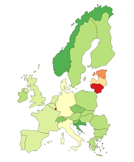
In addition to considering total system costs at the European level, the levelized cost of electricity
(LCoE) can also be examined at the country level. The levelized costs are calculated by dividing
the annualized total costs per country by the total amount of produced electricity per country
country country
(∑ coststotal,annualized / ∑ electricity produced ). For this purpose, the LCoE for the modeled countries
are given in Figure 7. The corresponding data for the figure can be found in Appendix A Table A1.
The LCoE range between 2.6 and 20.0 Cent/kWh in the four scenarios MonCap, MonCapShare,
EmiCap and EmiCapShare for most countries. Only in a few exceptions the LCoE are above
20.0 Cent/kWh, like Luxembourg in the EmiCap scenario. Norway has low LCoE in all four
scenarios with 2.6–2.7 Cent/kWh. In contrast, Lithuania has high LCoE in all scenarios with values
of 31.1–33.5 Cent/kWh. The high LCoE for the Baltic States are noticeable. When the MonCapShare
scenario is compared with the EmiCapShare scenario, only a minor difference can be observed.
Compared to the MonCapShare scenario, the LCoEs in the MonCap scenario change in Germany,
Denmark, Belgium, Greece and Estonia. On the one hand, in Denmark, Belgium and Greece the LCoE
in the MonCap scenario are higher than in the MonCapShare scenario. On the other hand, for Germany
and Estonia the value in the MonCap scenario is lower, from 10.5 Cent/kWh to 9.8 Cent/kWh and
from 17.3 Cent/kWh to 12.7 Cent/kWh. The LCoE in Estonia fall by 4.6 Cent/kWh between the
EmiCap and the EmiCapShare scenario. Other countries whose LCoEs differ between the EmiCap and
the EmiCapShare scenario are Germany, Denmark, Greece, Luxembourg and Portugal. The LCoE in
Denmark and Luxembourg are increasing. In Luxembourg the increase is quite high with an increase
from 11.1 Cent/kWh in the EmiCap scenario to 49.0 Cent/kWh. In Germany, Greece and Portugal,
the LCoE drop. In comparison, the LCoE in Sweden, Norway and Finland are robust and differ only
slightly between the individual scenarios. An overview of the amount of electricity produced for each
country can be found in the Appendix A (Tables A2–A5).Energies 2020, 13, 718 12 of 22
MonCap MonCapShare
0–2
2–4
4–6
6–8
8 – 10
[ct2015/kWh]
EmiCap EmiCapShare
10 – 12
12 – 14
14 – 16
16 – 18
18 – 20
> 20
Figure 7. Levelized cost of electricity for the modeled region for given scenarios.
5. Discussion
The scenario analysis allows a variety of insights. This section discusses what explanations
might be given for the nature of the results regarding installed capacities and generated electricity.
The significance of the cost and emission results of the individual scenarios will also be examined.
Finally, it is explored what influences the levelized cost of electricity and why different regions are
affected differently.
The solution of the MonFlex calculation shows a high installed capacity for hydro because of
its low costs. Furthermore, hydro is being used with a high load factor of 86.3%. In comparison,
the load factor in the calibrated CapShare scenarios is less than half at 37.5%. Therefore, it has to be
noted that the high amount of electricity generated by hydro in the MonFlex scenario is not reasonable
under real world circumstances. The amount of water available for electricity generation is in the
real world limited by external factors, e.g., melt-water. When interpreting the results for the EmiFlex
scenario, the statements from Section 4 should be kept in mind. The objective for this calculation is
the minimization of CO2 emissions. Because several technologies exist that do not emit CO2 , there
is a wide solution space. The solution found here is only one of many and is most likely not the
cost-optimal. The installed capacities in the remaining scenarios are the same due to the fact that
these are given to the model as input as they represent the European power plant fleet from 2015 (cf.
Section 2).
The results show a difference in the absolute amount of electricity generated, while the absolute
electricity demand stays constant , because it is a model input. The amounts of produced electricity
differ in fact between the scenarios due to the different use of storage technologies, like pumpstorages.Energies 2020, 13, 718 13 of 22
Since these technologies have an efficiency of less than one, electricity is lost during charging and
discharging. To compensate for this, more electricity has to be produced than if the electricity would
have not be stored.
The following findings can be derived from the results for electricity generation and the utilization
of the European power plant fleet. In the MonFlex calculation, for example, hydro power plants are the
main source of electricity because they are associated with low levelized cost of electricity (LCoE) while
natural constraints (e.g., water availability, feasibility of installations) are neglected. Gas is used, in
addition to hydro, in this scenario. Gas is chosen as a second technology to fill the gap between demand
and generation by hydro, because it has low investment costs compared to the other technologies (cf.
Appendix A Table A6). Electricity production and load factors in the MonCapShare and EmiCapShare
scenarios are almost identical. The remaining differences for electricity production can be explained
by the remaining solution space. Since the capacities are specified in the two CapShare scenarios,
the marginal production costs are pivotal for the selection of technologies needed to meet the electricity
demand. Depending on the objective function, the cheapest technologies available are selected in
the MonCapShare calculation and the technologies with lowest specific CO2 emissions are selected
in the EmiCapShare calculation. Thus, in the MonCapShare scenario the load factor of hard coal is
10.4% higher (53.4% instead of 43.0%) but that of gas 5.4% lower (18.1% instead of 23.5%) than in
the EmiCapShare scenario. In the MonCap scenario technologies with low fuel costs such as lignite,
nuclear and biomass are used to their full capacity. Technologies with high fuel costs such as gas
and hard coal are used less in comparison to the CapShare calculations. Oil is not used for electricity
production. For the EmiCap calculation, the technologies are used according to their specific CO2
emissions. Biomass and nuclear have particularly high load factors of 99.7% and 91.1%, respectively.
Local bottlenecks and fully utilized interconnector capacities prevent a load factor of 100%. For fossil
fuel based technologies, gas makes the largest contribution to electricity generation. Of the remaining
fossil fuel technologies, only hard coal contributes to electricity generation, accounting for 2.5% of total
electricity production. Oil and lignite are not used at all due to their high specific CO2 emissions. The
difference in load factors for hydro between the Cap and the CapShare scenarios can be explained by
the fact that hydro does not have a production share constraint for all countries.
The results of the MonCapShare and EmiCapShare calcuations are closest to real world data due
to the input data and constraints of the model and deviate only slightly from the statistic values (cf.
Section 4). While the total system costs and total emissions of the MonCap scenario are similar to those
of the CapShare scenarios, there are some differences. One factor for the difference to the statistical
data are technical restrictions that are not implemented in the model. Furthermore, all capacities in
the model are primarily used for electricity generation. Plants which in reality are heat-operated or
driven by industrial demand are modeled as electricity-operated. While some technologies in the
model produce heat as well, their primary task is to cover the electricity demand. In reality, however,
industrial power plants exist that cover a demand for process heat and their electricity generation is
only of secondary interest. Another factor for the deviations is that no electricity market mechanisms,
such as balancing power, are reflected in the model.
The comparison of total system costs and total CO2 emissions show that for the MonFlex scenario
the annualized total system costs are as low as expected, while the CO2 emissions for this scenario are
low, although the objective is total system costs. However, this result is purely academic in nature, as
the calculated capacity and quantity of electricity produced by hydro is not reasonable. The reason why
the values of total system costs and total emissions are not identical for the two CapShare calculations
is, as already described above, due to the remaining solution space of the optimization. The fact that
the results of the MonCap scenario are close to the ones of the MonCapShare scenario shows that there
is little optimization potential in terms of total system costs. This is mainly due to the high share of
investment costs in total system costs , which are only dependent on the installed capacities and are
model inputs. That is why it is more informative to examine the fuel costs. The potential saving by
a different operation of the existing European power plant fleet in fuel costs for the MonCap scenarioEnergies 2020, 13, 718 14 of 22
are 36.3% compared to the ones in the MonCapShare scenario. It should be noted that technical
limitations and market mechanisms, e.g., ramping constraints and minimum power, are neglected in
the model. Therefore the real savings potential is lower. The similar comparison between the EmiCap
and the EmiCapShare scenario shows that there is a large savings potential for CO2 emissions.
The results clearly show, that there is a great potential to reduce the total CO2 emissions of
power generation with the existing European power plant fleet at comparable low additional total
system costs. The total system costs of the EmiCap scenario is higher than those of the EmiCapShare
scenario, but only by 5.0%. The fuel costs are about 37.2% higher in the EmiCap scenario than in the
EmiCapShare scenario. The savings potential of total CO2 emissions is therefore not only high, there
are also only minor additional total system costs.
However, this result has different effects on the levelized cost of electricity (LCoE) in the modeled
countries. The changes in the LCoE are mainly due to two effects. The first effect is the different
utilization of technologies between scenarios due to the underlying objective function and constraints.
Thus in the MonCap scenario expensive electricity from technologies such as gas and oil is replaced by
less expensive electricity from technologies such as hard coal, biomass or hydro. Contrary, the capacity
utilization in the EmiCap scenario is determined by the specific CO2 emissions of the different
technologies. Therefore, more technologies with low specific CO2 emissions such as biomass, gas,
hydro or nuclear are used instead of technologies such as hard coal, lignite and oil. However, this may
lead to a higher utilization of technologies that are more expensive. The second effect, why the LCoE
differ in the scenarios, is the electricity production in the respective countries. In some countries,
like Bulgaria, the amount of electricity produced in the MonCap scenario is smaller than in the
MonCapShare scenario. In other countries it is the other way round. The reason why the quantities of
electricity produced in countries differ between the individual scenarios is due to the combination
of the composition of the respective power plants, the objective function and the capacities of the
interconnectors. The interaction of cost of technologies and generated electricity on the LCoE is not
always straightforward, as the dominating driver may vary from one country to another. For example,
in Germany more gas and oil are used in the MonCapShare scenario and less hard coal, lignite, biomass
and hydro than in the MonCap scenario. In addition, electricity production in Germany is higher in the
MonCapShare scenario with 532.9 TWh/a than in the MonCap scenario with 481.2 TWh/a. As a result,
the LCoE for Germany in the MonCapShare scenario with 9.8 Cent/kWh are lower than in the MonCap
scenario where the LCoE for Germany is 10.5 Cent/kWh. The effect of utilizing more expensive
technologies in Germany is therefore smaller than the effect of increased electricity production. For
regions like Denmark West exactly the opposite is the case. Here the additional electricity production
is too low to cancel out the effect of the more expensive technologies chosen, which is why the LCoE
are higher in the MonCapShare scenario than in the MonCap scenario. The impact of the two effects
on the LCoE is particularly evident for the LCoE of Luxembourg for the comparision of the EmiCap
and EmiCapShare scenarios. Here the expensive and emission-rich technology oil is used more in the
EmiCapShare scenario than in the EmiCap scenario. Contrary, in the EmiCap scenario more biomass,
gas and hydro is used than in the EmiCapShare scenario. At the same time, the amount of electricity
produced in the EmiCap scenario (4.2 TWh/a) is 5.7 times higher than in the EmiCapShare scenario
(0.7 TWh/a). Overall, this leads to a decrease of the LCoE for Luxembourg from 49.0 Cent/kWh in
the EmiCapShare scenario to 11.1 Cent/kWh in the EmiCap scenario. This can be explained by the
fact that instead of expensive technology less expensive technologies are used while the amount of
electricity produced increases.
The extent to which the LCoE differ between the scenarios depends on the use of the technologies
and the amount of electricity produced in the countries. The focus on technologies with low specific
CO2 emissions in the EmiCap scenario, for example, does cause additional total system costs. However,
not all countries are affected to the same extent. As expected, the LCoE increase in some countries
compared to the LCoE in the EmiCapShare scenario. However, there are also countries like Belgium,Energies 2020, 13, 718 15 of 22
Italy or Luxembourg in which the LCoE as well as the CO2 emissions decrease between the two
scenarios. These countries profit twice from an optimization in regards to CO2 emissions.
6. Conclusions
Climate change causes energy policy makers in Europe and around the world to think about
measures to decrease green house gas emissions. The European power plant fleet contributes
significantly to the greenhouse gas emissions in Europe and, hence, is a possible object for reduction
activities. Energy policy makers and energy system analysts need an estimation for the reduction
potential that could be realized with the existing European power plant fleet and what are related costs.
In this study the model of the European electricity system Stella is introduced. The implementation
is carried out in Calliope, an open-source modeling framework programmed in Python. The model
covers 29 European regions, which are represented in 29 interconnected nodes. A given time series of
electricity demand is covered by thermal or renewable generation technologies during the solution
process. Objective function is minimization of either annualized total system costs or CO2 emissions.
To achieve the goal of this study, six scenarios have been developed. Two scenarios cover the electricity
demand for 2015 in an unconstrained way minimizing either total system costs or total emissions.
In four additional scenarios the European power plant capacities are imprinted on the model, which
means that investment costs have no impact on the optimization. In two of these four scenarios
historical production values are fixed enabling a comparison of historical and potential values.
The scenario results show that the greenhouse gas emissions of the European power plant fleet
could be reduced potentially by more than 50% with low additional total system costs of around 5%
resulting in relative low specific CO2 abatement costs. The results further show that today’s operation
strategy of the European power plant fleet is close to a cost optimal manner. Hence, the results
prove the economic manner of today’s power plant operation with only little consideration of its
corresponding climate influence.
The results motivate further research in how to establish incentives for energy suppliers to
generate more electricity from climate friendly electricity sources. For investigation, the constraints
of heat-operated power plants in the industrial and public power plants could be examined and
included in the model. To set up the model a lot of input data is required. Data is often specified with
a bandwidth. However, exact values are required as model inputs. In a future study this issue can be
addressed by performing a sensitivity analysis, which shows the influence of different parameters on
the results. Finally, the results could be checked for robustness, for example by using solar and wind
data from multiple years.
Author Contributions: Conceptualization, B.-J.J., S.M., B.G. and S.B.; Data curation, B.-J.J., S.M., B.G. and S.B.;
Investigation, B.-J.J., S.M., B.G. and S.B.; Methodology, B.-J.J., S.M., B.G. and S.B.; Software, B.-J.J., S.M., B.G.
and S.B.; Supervision, W.K.; Validation, B.-J.J., S.M., B.G. and S.B.; Visualization, B.-J.J., S.M., B.G. and S.B.;
Writing—original draft, B.-J.J., S.M., B.G. and S.B.; Writing—review & editing, B.-J.J., S.M., B.G., S.B. and W.K.
All authors have read and agree to the published version of the manuscript.
Funding: This research received no external funding.
Conflicts of Interest: The authors declare no conflict of interest.Energies 2020, 13, 718 16 of 22
Appendix A
Table A1. Levelized cost of electricity by scenario and country [Cent2015 /kWh].
MonCap MonCapShare EmiCap EmiCapShare
Austria (AT) 7.7 9.6 6.4 9.0
Belgium (BE) 9.6 13.8 8.7 13.1
Bulgaria (BG) 7.3 6.4 12.7 8.0
Switzerland (CH) 4.3 4.5 4.1 4.5
Czechia (CZ) 5.9 7.8 13.0 9.1
Germany (DE) 10.5 9.8 12.7 9.7
Denmark—East (DKE) 11.5 12.0 12.6 11.9
Denmark—West (DKW) 11.5 13.2 10.6 13.1
Estonia (EE) 17.3 12.7 17.3 12.7
Spain (ES) 8.7 9.7 9.4 9.4
Finland (FI) 6.2 7.0 6.7 6.9
France (FR) 8.4 9.7 8.2 9.7
Great Britain (GB) 8.5 9.0 8.9 8.6
Greece (GR) 7.3 10.3 12.1 10.1
Croatia (HR) 4.0 3.9 4.0 3.9
Hungary (HU) 7.2 8.8 7.4 8.2
Ireland (IE) 6.5 7.0 8.0 7.0
Italy (IT) 10.3 10.6 9.8 10.1
Lithuania (LT) 34.1 33.5 31.1 33.5
Luxembourg (LU) 46.6 57.3 11.1 49.0
Latvia (LV) 12.4 15.6 12.4 15.6
Netherlands (NL) 9.7 8.5 7.9 8.0
Norway (NO) 2.6 2.7 2.6 2.7
Poland (PL) 6.3 5.3 8.3 7.4
Portugal (PT) 8.3 8.7 10.9 8.9
Romania (RO) 6.6 8.7 12.2 8.7
Sweden (SE) 7.4 7.3 7.4 7.3
Slovenia (SI) 5.4 7.4 8.2 7.4
Slovakia (SK) 6.2 6.7 6.5 6.7
Table A2. Electricity generation [TWh/a]—MonCap.
Biomass Gas Hard Coal Hydro Lignite Nuclear Oil Other Solar Wind
AT 10.4 0.0 0.7 38.5 0.0 0.0 0.0 0.1 1.2 5.7
BE 7.2 1.1 2.1 1.7 0.0 51.1 0.0 0.0 3.5 5.4
BG 0.5 0.0 0.0 5.7 32.1 4.2 0.0 0.0 1.4 1.4
CH 2.7 0.0 0.0 112.5 0.0 23.7 0.0 0.0 2.3 0.1
CZ 6.6 0.0 0.2 2.3 73.3 21.9 0.0 0.0 2.5 0.6
DE 63.1 0.0 17.7 19.6 163.2 89.1 0.0 0.3 43.9 84.3
DKE 4.7 0.0 1.2 0.0 0.0 0.0 0.0 0.0 0.3 4.4
DKW 4.7 0.0 0.4 0.0 0.0 0.0 0.0 0.0 0.5 9.5
EE 1.5 0.0 0.0 0.0 0.0 0.0 0.0 0.0 0.0 0.7
ES 7.9 3.9 57.4 31.6 26.4 66.3 0.0 0.0 7.2 50.4
FI 16.7 0.0 14.4 16.6 0.0 24.3 0.0 0.1 0.0 3.1
FR 7.0 0.0 0.4 55.2 0.0 510.3 0.0 0.0 8.4 22.5Energies 2020, 13, 718 17 of 22
Table A2. Cont.
Biomass Gas Hard Coal Hydro Lignite Nuclear Oil Other Solar Wind
GB 37.7 16.6 105.6 9.7 0.0 78.1 0.0 0.0 8.8 43.9
GR 0.4 0.1 0.0 1.5 39.9 0.0 0.0 0.0 3.7 4.9
HR 0.5 0.0 0.0 15.2 0.0 0.0 0.0 0.0 0.1 0.5
HU 4.3 0.0 0.1 0.2 8.8 15.3 0.0 0.0 0.2 0.7
IE 0.5 5.5 8.0 1.2 2.2 0.0 0.0 0.0 0.0 6.8
IT 25.9 51.8 74.9 44.3 0.0 0.0 0.0 0.9 25.7 13.8
LT 0.6 0.0 0.0 0.3 0.0 0.0 0.0 0.0 0.1 1.1
LU 0.1 0.0 0.0 0.3 0.0 0.0 0.0 0.0 0.1 0.1
LV 1.1 0.0 0.0 1.9 0.0 0.0 0.0 0.0 0.0 0.2
NL 4.7 4.0 31.3 0.1 0.0 4.3 0.0 0.9 1.7 8.0
NO 0.0 0.0 0.0 201.9 0.0 0.0 0.0 0.0 0.0 2.2
PL 8.4 0.0 23.7 2.7 82.9 0.0 0.0 0.0 0.1 11.1
PT 4.7 2.1 15.3 9.5 0.0 0.0 0.0 0.0 0.7 11.1
RO 1.0 0.0 0.0 16.5 41.0 4.1 0.0 0.0 1.6 6.5
SE 37.5 0.0 0.0 74.0 0.0 23.8 0.0 0.0 0.1 15.5
SI 0.5 0.0 0.0 3.9 8.3 6.3 0.0 0.0 0.3 0.0
SK 2.1 0.0 0.0 12.9 4.3 15.7 0.0 0.0 0.6 0.0
Table A3. Electricity generation [TWh/a]—MonCapShare.
Biomass Gas Hard Coal Hydro Lignite Nuclear Oil Other Solar Wind
AT 3.3 0.6 3.8 32.5 0.0 0.0 1.1 0.1 1.2 5.7
BE 3.0 7.6 4.1 0.3 0.0 26.1 0.2 0.0 3.5 5.4
BG 0.2 1.3 14.0 5.7 18.7 14.3 0.0 0.0 1.4 1.4
CH 0.1 0.1 0.0 110.4 0.0 22.9 0.0 0.0 2.3 0.1
CZ 2.0 5.0 15.4 1.8 33.4 25.8 0.0 0.0 2.5 0.6
DE 39.3 0.4 110.5 16.1 145.0 87.9 5.6 0.3 43.7 84.1
DKE 0.4 0.0 5.5 0.0 0.0 0.0 0.0 0.0 0.3 4.4
DKW 1.9 0.1 1.3 0.0 0.0 0.0 0.1 0.0 0.5 9.5
EE 1.3 0.0 0.0 0.0 0.0 0.0 5.9 0.0 0.0 0.7
ES 4.6 39.1 48.6 27.5 4.5 54.8 13.0 0.0 7.2 50.3
FI 11.1 9.6 6.3 16.6 0.0 22.9 0.5 0.1 0.0 3.1
FR 7.0 0.8 8.6 53.7 0.0 416.1 3.4 0.0 8.4 22.5
GB 0.1 87.4 95.0 4.7 0.0 65.7 0.0 0.0 8.8 43.7
GR 0.2 8.9 0.0 0.7 19.8 0.0 0.1 0.0 3.7 4.9
HR 0.0 0.8 2.1 15.0 0.0 0.0 0.0 0.0 0.1 0.5
HU 1.6 0.1 0.5 0.2 5.6 15.0 0.0 0.0 0.2 0.7
IE 0.0 8.5 4.9 1.1 2.2 0.0 0.1 0.0 0.0 6.8
IT 20.1 92.7 42.3 43.2 0.0 0.0 6.4 0.9 25.7 13.7
LT 0.4 0.2 0.0 0.3 0.0 0.0 0.0 0.0 0.1 1.1
LU 0.1 0.1 0.0 0.1 0.0 0.0 0.0 0.0 0.1 0.1
LV 0.4 0.0 0.0 1.9 0.0 0.0 0.0 0.0 0.0 0.2
NL 4.7 29.8 21.5 0.1 0.0 4.3 0.1 0.9 1.6 8.0
NO 0.0 3.5 0.0 195.6 0.0 0.0 0.0 0.0 0.0 2.2
PL 7.0 4.5 106.0 1.8 52.1 0.0 0.2 0.0 0.1 11.1
PT 2.6 5.4 13.7 8.5 0.0 0.0 0.1 0.0 0.7 11.0
RO 0.5 0.0 2.1 16.5 15.7 11.0 0.3 0.0 1.6 6.5
SE 10.0 1.1 0.5 74.4 0.0 54.8 0.0 0.0 0.1 15.5
SI 0.2 0.0 0.0 3.8 3.9 5.5 0.0 0.0 0.3 0.0
SK 1.1 1.9 1.0 12.7 1.7 14.4 0.0 0.0 0.6 0.0Energies 2020, 13, 718 18 of 22
Table A4. Electricity generation [TWh/a]—EmiCap.
Biomass Gas Hard Coal Hydro Lignite Nuclear Oil Other Solar Wind
AT 10.4 32.7 0.0 37.2 0.0 0.0 0.0 0.1 1.2 5.7
BE 7.2 16.8 0.0 1.2 0.0 51.3 0.0 0.0 3.5 5.4
BG 0.5 0.2 0.0 5.7 0.0 17.1 0.0 0.0 1.4 1.4
CH 2.7 0.0 0.0 117.5 0.0 25.6 0.0 0.0 2.3 0.1
CZ 6.6 2.6 0.0 2.4 0.0 33.9 0.0 0.0 2.5 0.6
DE 63.1 119.0 0.1 20.5 0.0 94.6 0.0 0.3 43.9 84.3
DKE 4.7 0.3 0.0 0.0 0.0 0.0 0.0 0.0 0.3 4.4
DKW 4.7 2.7 0.0 0.0 0.0 0.0 0.0 0.0 0.5 9.5
EE 1.5 0.0 0.0 0.0 0.0 0.0 0.0 0.0 0.0 0.7
ES 7.9 98.1 0.0 27.7 0.0 66.3 0.0 0.0 7.2 50.4
FI 16.7 12.2 0.0 16.6 0.0 24.3 0.0 0.1 0.0 3.1
FR 7.0 0.5 0.0 62.2 0.0 519.8 0.0 0.0 8.4 22.5
GB 37.7 141.9 0.0 5.3 0.0 78.1 0.0 0.0 8.8 43.9
GR 0.4 28.9 0.0 0.7 0.0 0.0 0.0 0.0 3.7 4.9
HR 0.5 0.7 0.0 15.1 0.0 0.0 0.0 0.0 0.1 0.5
HU 4.3 12.7 0.0 0.2 0.0 16.6 0.0 0.0 0.2 0.7
IE 0.5 14.4 0.0 1.0 0.0 0.0 0.0 0.0 0.0 6.8
IT 25.9 166.4 0.0 43.9 0.0 0.0 0.0 0.9 25.7 13.8
LT 0.6 0.2 0.0 0.3 0.0 0.0 0.0 0.0 0.1 1.1
LU 0.1 3.2 0.0 0.6 0.0 0.0 0.0 0.0 0.1 0.1
LV 1.1 0.0 0.0 1.9 0.0 0.0 0.0 0.0 0.0 0.2
NL 4.7 74.2 0.0 0.1 0.0 4.3 0.0 0.9 1.7 8.0
NO 0.0 0.0 0.0 201.9 0.0 0.0 0.0 0.0 0.0 2.2
PL 8.4 11.4 80.7 1.8 0.0 0.0 0.0 0.0 0.1 11.1
PT 4.7 7.0 0.0 8.5 0.0 0.0 0.0 0.0 0.7 11.1
RO 1.0 0.1 0.0 16.5 0.0 11.7 0.0 0.0 1.6 6.5
SE 37.5 0.0 0.0 74.1 0.0 24.0 0.0 0.0 0.1 15.5
SI 0.5 2.7 0.0 3.8 0.0 6.4 0.0 0.0 0.3 0.0
SK 2.1 2.5 0.0 13.0 0.0 17.0 0.0 0.0 0.6 0.0
Table A5. Electricity generation [TWh/a]—EmiCapShare.
Biomass Gas Hard Coal Hydro Lignite Nuclear Oil Other Solar Wind
AT 3.3 6.6 3.8 32.5 0.0 0.0 1.1 0.1 1.2 5.7
BE 3.0 11.0 4.1 0.3 0.0 26.1 0.2 0.0 3.5 5.4
BG 0.2 1.3 0.0 5.7 18.7 14.3 0.0 0.0 1.4 1.4
CH 0.1 0.1 0.0 110.4 0.0 22.9 0.0 0.0 2.3 0.1
CZ 2.0 5.0 0.0 1.8 33.4 25.8 0.0 0.0 2.5 0.6
DE 39.3 13.0 110.5 16.1 145.0 87.9 5.6 0.3 43.7 84.1
DKE 0.5 0.0 5.6 0.0 0.0 0.0 0.0 0.0 0.3 4.4
DKW 1.8 0.4 1.3 0.0 0.0 0.0 0.1 0.0 0.5 9.5
EE 1.3 0.0 0.0 0.0 0.0 0.0 5.9 0.0 0.0 0.7
ES 4.6 52.7 48.6 27.5 4.5 54.8 13.0 0.0 7.2 50.3
FI 11.1 12.2 6.3 16.6 0.0 22.9 0.5 0.1 0.0 3.1
FR 7.0 4.3 8.6 53.7 0.0 416.1 3.4 0.0 8.4 22.5
GB 0.1 107.7 95.0 4.7 0.0 65.7 0.0 0.0 8.8 43.7
GR 0.2 10.0 0.0 0.7 19.8 0.0 0.1 0.0 3.7 4.9
HR 0.0 0.8 2.1 15.0 0.0 0.0 0.0 0.0 0.1 0.5
HU 1.6 3.1 0.5 0.2 5.6 15.0 0.0 0.0 0.2 0.7
IE 0.0 8.1 4.9 1.1 2.2 0.0 0.1 0.0 0.0 6.8
IT 20.1 113.0 42.3 43.2 0.0 0.0 6.4 0.9 25.7 13.7
LT 0.4 0.2 0.0 0.3 0.0 0.0 0.0 0.0 0.1 1.1
LU 0.1 0.3 0.0 0.1 0.0 0.0 0.0 0.0 0.1 0.1
LV 0.4 0.0 0.0 1.9 0.0 0.0 0.0 0.0 0.0 0.2
NL 4.7 37.4 21.5 0.1 0.0 4.3 0.1 0.9 1.6 8.0
NO 0.0 3.5 0.0 195.6 0.0 0.0 0.0 0.0 0.0 2.2Energies 2020, 13, 718 19 of 22
Table A5. Cont.
Biomass Gas Hard Coal Hydro Lignite Nuclear Oil Other Solar Wind
PL 7.0 4.5 36.7 1.8 52.1 0.0 0.2 0.0 0.1 11.1
PT 2.6 4.0 13.7 8.5 0.0 0.0 0.1 0.0 0.7 11.0
RO 0.5 0.0 2.1 16.5 15.7 11.0 0.3 0.0 1.6 6.5
SE 10.0 1.1 0.5 74.4 0.0 54.8 0.0 0.0 0.1 15.5
SI 0.2 0.0 0.0 3.8 3.9 5.5 0.0 0.0 0.3 0.0
SK 1.1 1.9 1.0 12.7 1.7 14.4 0.0 0.0 0.6 0.0
Table A6. Techno-economic parameters which are used as model input data for all scenarios.
Fuel Group Investment Cost O&M Cost Lifetime Efficiency
[e2015 /kW] [e2015 /kW] [a] [%]
ConELC-PP_COA Hard Coal 1365 27 45 35
ConELC-PP_LIG Lignite 1552 33 45 35
ConELC-PP_NG-OCGT Gas 568 17 40 45
ConELC-PP_NG-ST Gas 750 19 40 30
ConELC-PP_NG-CCGT Gas 855 26 40 60
ConELC-PP_OIL Oil 750 20 40 25
ConELC-PP_NUC Nuclear 5000 43 50 33
ConELC-PP_BIO Biomass 2306 92 25 28
ConELC-PP_HYD-ROR Hydro 1454 15 200 –
ConELC-PP_HYD-STO Hydro 1385 28 200 –
ConELC-PP_HYD-PST Hydro 1385 28 200 86.6
ConELC-PP_WON Wind 1400 34 25 –
ConELC-PP_WOF Wind 3000 106 25 –
ConELC-PP_SPV Solar 3378 51 25 –
ConELC-PP_CSP Solar 5200 104 25 –
ConELC-PP_GEO Other 2400 84 30 –
ConELC-PP_WST Other 2530 51 30 –
ConELC-PP_OTH Other 5500 55 20 –
ConELC-CHP_COA Hard Coal 1646 33 45 40
ConELC-CHP_LIG Lignite 1872 40 45 30
ConELC-CHP_NG-OCGT Gas 568 17 40 40
ConELC-CHP_NG-ST Gas 1182 21 40 31
ConELC-CHP_NG-CCGT Gas 823 21 40 40
ConELC-CHP_OIL Oil 1182 20 40 10
ConELC-CHP_BIO Biomass 2306 0 25 40
ConELC-CHP_GEO Other 2400 84 25 –
ConELC-CHP_WST Other 2530 51 30 –
ConELC-CHP_OTH Other 5500 55 20 –
Table A7. Cost and emission data for fuels which are used as model input data for all scenarios.
Cost Emissions
[e2015 /kWhfuel ] [kgCO2 /kWhfuel ]
Biomass Supply 0.001 0
Crude Oil Supply 0.0260 0.2786
Electricity Supply (outer regions) 0.3 0.5
Hard Coal Supply 0.0061 0.3406
Lignite Supply 0.0013 0.3643
Natural Gas Supply 0.0207 0.2020
Uranium Supply 0.0033 0.0050Energies 2020, 13, 718 20 of 22
1.00
0.75
0.50
0.25
Load factor
0.00
0.25
0.50
0.75
1.00 MonCapShare EmiCapShare
Figure A1. Deviation between CapShare scenarios and real world data for the load factor with outliers.
0.100
0.075
Electricity generation [TWh/a]
0.050
0.025
0.000
0.025
0.050
0.075
0.100 MonCapShare EmiCapShare
Figure A2. Deviation between CapShare scenarios and real world data for the generated electricity.
100
Electricity generation [TWh/a]
50
0
50
100
MonCapShare EmiCapShare
Figure A3. Deviation between CapShare scenarios and real world data for the generated electricity
with outliers.Energies 2020, 13, 718 21 of 22
References
1. Intergovernmental Panel on Climate Change (IPCC). Summary for Policymakers. In Global Warming of
1.5 ◦ C. An IPCC Special Report on the Impacts of Global Warming of 1.5 ◦ C above Pre-Industrial Levels and Related
Global Greenhouse Gas Emission Pathways, in the Context of Strengthening the Global Response to the Threat of
Climate Change, Sustainable Development, and Efforts to Eradicate Poverty; IPCC: Geneva, Switzerland, 2018.
2. Federal Ministry for Economic Affairs and Energy (BMWi). Innovation durch Forschung—Erneuerbare Energien
und Energieeffizienz: Projekte und Ergebnisse der Forschungsförderung 2018; Federal Ministry for Economic
Affairs and Energy (BMWi): Berlin, Germany, 2019.
3. European Environment Agency (EEA). Adaptation Challenges and Opportunities for the European Energy System;
European Environment Agency: Copenhagen, Denmark, 2019.
4. Pérez-Andreu, V.; Aparicio-Fernández, C.; Martínez-Ibernón, A.; Vivancos, J.L. Impact of climate change
on heating and cooling energy demand in a residential building in a Mediterranean climate. Energy 2018,
165, 63–74. [CrossRef]
5. Hueging, H.; Haas, R.; Born, K.; Jacob, D.; Pinto, J.G. Regional Changes in Wind Energy Potential over
Europe Using Regional Climate Model Ensemble Projections. J. Appl. Meteorol. Climatol. 2013, 52, 903–917.
[CrossRef]
6. Löffler, K.; Hainsch, K.; Burandt, T.; Oei, P.Y.; Kemfert, C.; von Hirschhausen, C. Designing a Model for
the Global Energy System—GENeSYS-MOD: An Application of the Open-Source Energy Modeling System
(OSeMOSYS). Energies 2017, 10, 1468. [CrossRef]
7. Pursiheimo, E.; Holttinen, H.; Koljonen, T. Inter-sectoral effects of high renewable energy share in global
energy system. Renew. Energy 2019, 136, 1119–1129. [CrossRef]
8. Fattori, F.; Albini, D.; Anglani, N. Proposing an open-source model for unconventional participation to
energy planning. Energy Res. Soc. Sci. 2016, 15, 12–33. [CrossRef]
9. Tahir, M.F.; Chen, H.; Javed, M.S.; Jameel, I.; Khan, A.; Adnan, S. Integration of Different Individual Heating
Scenarios and Energy Storages into Hybrid Energy System Model of China for 2030. Energies 2019, 12, 2083.
[CrossRef]
10. Heinrichs, H.U.; Markewitz, P. Long-term impacts of a coal phase-out in Germany as part of a greenhouse
gas mitigation strategy. Appl. Energy 2017, 192, 234–246. [CrossRef]
11. Pfenninger, S.; Pickering, B. Calliope: A multi-scale energy systems modelling framework. J. Open
Source Softw. 2018, 3, 825. [CrossRef]
12. Welder, L.; Ryberg, D.; Kotzur, L.; Grube, T.; Robinius, M.; Stolten, D. Spatio-temporal optimization of
a future energy system for power-to-hydrogen applications in Germany. Energy 2018, 158, 1130–1149.
[CrossRef]
13. Howells, M.; Rogner, H.; Strachan, N.; Heaps, C.; Huntington, H.; Kypreos, S.; Hughes, A.; Silveira, S.;
DeCarolis, J.; Bazillian, M.; et al. OSeMOSYS: The Open Source Energy Modeling System. Energy Policy
2011, 39, 5850–5870. [CrossRef]
14. Brown, T.; Hörsch, J.; Schlachtberger, D. PyPSA: Python for Power System Analysis. J. Open Res. Softw. 2018,
6. [CrossRef]
15. Hilpert, S.; Kaldemeyer, C.; Krien, U.; Günther, S.; Wingenbach, C.; Plessmann, G. The Open Energy
Modelling Framework (oemof)—A new approach to facilitate open science in energy system modelling.
Energy Strategy Rev. 2018, 22, 16–25. [CrossRef]
16. Richstein, J.C. Open Energy Modelling Initiative. 2019. Available online: https://www.openmod-initiative.
org (accessed on 17 October 2019).
17. Brown, T.; Schlachtberger, D.; Kies, A.; Schramm, S.; Greiner, M. Synergies of sector coupling and
transmission reinforcement in a cost-optimised, highly renewable European energy system. Energy 2018,
160, 720–739. [CrossRef]
18. Gerbaulet, C.; von Hirschhausen, C.; Kemfert, C.; Lorenz, C.; Oei, P.Y. European electricity sector
decarbonization under different levels of foresight. Renew. Energy 2019, 141, 973–987. [CrossRef]
19. Schlachtberger, D.; Brown, T.; Schäfer, M.; Schramm, S.; Greiner, M. Cost optimal scenarios of a future highly
renewable European electricity system: Exploring the influence of weather data, cost parameters and policy
constraints. Energy 2018, 163, 100–114. [CrossRef]You can also read