R 497 - An indicator of macro-financial stress for Italy by Arianna Miglietta and Fabrizio Venditti - Banca d'Italia
←
→
Page content transcription
If your browser does not render page correctly, please read the page content below
Questioni di Economia e Finanza
             (Occasional Papers)

             An indicator of macro-financial stress for Italy

             by Arianna Miglietta and Fabrizio Venditti
April 2019

                                                                         497
                                                                Number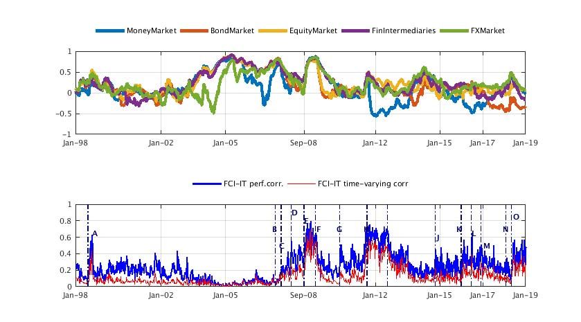
Questioni di Economia e Finanza
(Occasional Papers)

An indicator of macro-financial stress for Italy

by Arianna Miglietta and Fabrizio Venditti

Number 497 – April 2019
The series Occasional Papers presents studies and documents on issues pertaining to
the institutional tasks of the Bank of Italy and the Eurosystem. The Occasional Papers appear
alongside the Working Papers series which are specifically aimed at providing original contributions
to economic research.

                 The Occasional Papers include studies conducted within the Bank of Italy, sometimes
in cooperation with the Eurosystem or other institutions. The views expressed in the studies are those of
the authors and do not involve the responsibility of the institutions to which they belong.

                 The series is available online at www.bancaditalia.it .

ISSN 1972-6627 (print)
ISSN 1972-6643 (online)

Printed by the Printing and Publishing Division of the Bank of Italy
AN INDICATOR OF MACRO-FINANCIAL STRESS FOR ITALY
by Arianna Miglietta* and Fabrizio Venditti**
Abstract
We develop a measure of systemic stress for the Italian financial markets (FCI-IT) that
aggregates information from five major segments of the whole financial system, i.e. the
money market, the bond market, the equity market, the foreign exchange market and the
market for stocks of financial intermediaries. The index builds on the methodology of the
Composite Indicator of Systemic Stress (CISS) developed by Hollò, Kremer and Lo Duca
(2012) for the euro area. We set up a simple TVAR model to verify whether the proposed
measure is able to provide significant and consistent information about the evolution of
macroeconomic variables when financial conditions change. The indicator’s performance is
evaluated against two alternative metrics publicly available (e.g. the euro-area CISS and the
Italian CLIFS). Our results show that FCI-IT behaves quite similarly to the other indexes
considered in signalling high-stress periods, but it also identifies episodes of financial distress
for the Italian economy which are disregarded by the other two. During periods of high stress,
the effects of financial shocks on gross domestic product are significant.
JEL Classification: G01, G10, G20, E44
Keywords: Financial stability, systemic risk, financial condition index
Contents
1. Introduction ........................................................................................................................... 5
2. Data selection ........................................................................................................................ 7
3. The methodological framework ............................................................................................ 9
4. Results ................................................................................................................................. 11
5. Feedback loop between the Italian financial sector and the real sector:
a TVAR approach ................................................................................................................ 15
6. Conclusions .......................................................................................................................... 21
Appendix: Supplementary charts ............................................................................................. 22
References ................................................................................................................................ 26
_______________________________________
* Bank of Italy, Directorate General for Economics, Statistics and Research.
** European Central bank, Directorate General International and European Relations.Introduction
This note develops a measure of systemic stress for the Italian financial markets that aggregates
information from five major segments of the whole financial system, i.e. the money market, the
bond market, the equity market, the foreign exchange market and the market for stocks of financial
intermediaries. Specifically, the new index comprises 13 market-based indicators of financial stress
that originate from these five segments, and adapts to the Italian economy the Composite Indicator
of Systemic Stress (CISS) developed by Hollò, Kremer and Lo Duca (2012) for the euro area.
Unlike Iachini and Nobili (2014), who have developed an indicator of systemic liquidity risk for the
Italian financial markets, our index provides an assessment of financial distress from a broader
perspective.1 In order to verify whether the index can pinpoint episodes of stress in the financial
system that had significant consequences for economic activity, we developed a simple joint model
of our index and Italian GDP and show that, in periods of high stress, an innovation to the index is
associated with a significant economic downturn.
The post-crisis macro-financial literature has provided substantial evidence on the link between
financial stability and macroeconomic performance (for instance, Giglio, Kelly and Pruitt, 2016;
Adrian, Boyarchenko and Giannone, 2017). The financial crisis has shown that the financial sector
can be the source of strong shockwaves with disruptive consequences on the business cycle. When
faced with a large financial shock, the economy runs the risk of entering a vicious negative spiral
with financial and economic distress reinforcing each other.2 The crisis also revealed that financial
variables may have informative power about future GDP dynamics, over and above the information
contained in real variables, calling for the monitoring of financial stress and of the business cycle as
intertwined, rather than as isolated, phenomena. As a result, a large number of Financial Condition
Indexes (FCIs) has been developed in recent years to summarize in a single indicator the sometimes
conflicting signals from different segments of the financial system and to also provide information
on the future state of the economy.3
A FCI should be designed to evaluate the state of (in)stability within the financial system. Ideally,
such an index should not only identify in a time dimension the build-up of systemic imbalances
within the system (‘horizontal view’, ECB 2011), but also describe consistently the potential effects
1
The indicator developed in Iachini and Nobili (2014) provides an aggregate measure of systemic liquidity risk; three
segments of the Italian financial markets are covered, i.e. the equity and corporate market, the bond market and the
money market.
2
The mechanics underlying a standard ‘financial accelerator’ mechanism (see, e.g., Bernanke, Gertler and Gilchrist,
1999) could help explain how endogenous developments in financial markets could propagate and amplify shocks to the
real economy.
3
A non-exhaustive list of contributions on the topic includes Illing and Liu (2006), Cardarelli, Elekdag and Lall (2011),
Hakkio and Keeton (2009), Hatzius et al., (2010), Kliesen and Smith (2010), Matheson (2011), Brave and Butters
(2012), Hollò, Kremer and Lo Duca (2012), Koop and Korobilis (2014) and Iachini and Nobili (2014).
5of systemic distress when the interaction between the financial sector and the real economy is taken
into account (‘vertical view’, ECB 2011). In this respect, a FCI should capture the residual effect of
financial variables on the real economy once the direct impact of monetary policy changes has been
taken into account (Hatzius et al, 2010). Admittedly, this is not an easy task, also in light of the fact
that it is not easy to represent the complexity of the financial system through a single composite
measure; furthermore, financial innovation calls for a continuous updating of the indicators in order
to capture changes in the industry. An additional challenge faced when measuring financial
conditions is model instability. The financial/real economy nexus is not necessarily stable over
time, as it is shaped by developments in technological progress and financial innovation.4 Other
nonlinearities can arise from threshold effects such as, for instance, borrowing constraints or the
zero lower bound on interest rates.
Nonetheless, FCIs have their merits and may provide a valuable guide to policymakers to evaluate
financial conditions within an economy. In fact, a number of central banks have developed a FCI
which is included in the set of analytical instruments used to support their monetary and
macroprudential tasks, as well as their monitoring of financial stability (e.g. European Central
Bank, Bank of England, Federal Reserve, Bank of Canada, Bank of Portugal).5 In this note we take
a very similar approach to Hollò, Kremer and Lo Duca (2012), who have developed a Composite
Indicator of Systemic Stress (CISS) for the euro area. The resulting FCI for the Italian economy
moves closely with other financial condition indexes publicly available.6 This is not surprising,
given the evidence on the emergence of a ‘global financial cycle’ due to the increased integration
and openness of financial markets over the last decade (Rey, 2015; ECB, 2018). Despite this
correlation, we believe that the proposed indicator has some advantages in comparison to alternative
metrics. As with other comparable indexes, it identifies the most important episodes of stress
experienced in the last decade; it also points to further periods that have been particularly turbulent
for the Italian economy, decoupling from the other indicators considered.7 Moreover, it is able to
describe convincingly the interaction between the financial sector and the real economy. In general,
having an FCI tailored on the Italian financial system has some benefits. First, an in-house built
4
Hatzius et al., (2010) find that the predictive ability of their FCI for future GDP, relative to that of a simple
autoregressive benchmark, changes significantly over time. Hollò, Kremer and Lo Duca (2012) use a time-varying
cross-correlation structure to aggregate sub-indexes into a composite measure in order to put more weight on situations
in which there is a synchronous movement across markets.
5
FCIs have also been developed in the private sector (among others, Bloomberg, Deutsche Bank and Goldman Sachs).
6
In this note we consider the euro-area CISS and the Italian Country Level Index of Financial Stress (CLIFS; Duprey et
al., 2017). The first indicator is available weekly from the ECB Statistical Data Warehouse. The second one is instead
published with monthly frequency and focuses on three market segments only (i.e. equity market, bond market and
foreign exchange market); its information content is therefore less complete.
7
For instance, our index would flag the tensions in mid-May 2018 as a period of distress while the other two metrics
considered would remain in a ‘safe area’.
6metric of systemic distress allows a real-time monitoring of financial stability risks for the Italian
economy. Second, it can complement the indicators already included in the Risk Dashboard for the
Italian economy providing a composite and synthetic measure of financial conditions (Venditti et
al., 2018). Third, indicators of general systemic stress have been included by the ESRB among the
metrics to inform the judgment on the Countercyclical Capital Buffer during the release phase
(ESRB, 2014). From this perspective, the proposed indicator represents a first valuable step. Future
applications include, for instance, the broadening of the dataset to the infrastructure segment and the
shadow banking system and the refinement of the list of raw indicators by means of statistical
techniques.
The remainder of this note is organized as follows. Section 2 discusses the raw data used to
construct a FCI for Italy. Section 3 describes the statistical methodology. The results obtained are
illustrated in Section 4. Section 5 gauges whether the proposed measure is able to provide
significant information on the evolution of macroeconomic variables when financial conditions
change. Section 6 concludes.
2. Data selection
This section presents the data used in the construction of a FCI for the Italian economy. The idea
generally exploited in the creation of FCIs is that the financial system can be represented by three
segments: (i) financial markets, (ii) intermediaries and (iii) infrastructures. Starting from a standard
set of basic indicators, specific metrics can be computed for each segment (i.e. first level); they can
then be aggregated to provide a single measure of stress for each of the segments considered (i.e.
second level); a composite financial stress indicator for the whole financial system can finally be
obtained by using the data processed in the previous steps (i.e. third level). Notably, due to limited
data availability, most existing FCIs, including the one described in this note, neglect the
infrastructure block thus focusing on markets and intermediaries only. Integrating the dataset with
information on this group is left for future refinements of the indicator.
Based on the scheme illustrated above, we selected 5 representative market segments – i.e. the
money market, the bond market, the equity market, the foreign exchange market and the market for
stocks of financial intermediaries – which represent the bulk of most financial systems. The
selection of basic indicators is of crucial importance as they should be able to both identify key
patterns in the corresponding segment, and to capture signs of financial distress in real time, while
simultaneously providing complementary information within each segment. Therefore, we have
selected indicators based on market prices (rather than on quantities) due to both their long data
history and availability at daily/weekly frequency; in order to capture market-wide developments,
7market indices have been considered where appropriate. More detailed information on the raw data
and the metrics used is reported in Table 1.
Table 1
Description of the individual raw indicators by market segment
Market segments Source/Code Name of the variable
Money market
Volatility of the 3-month Euribor rate Datastream; code: vol-3MEur
Volatility calculated as the weekly average of absolute daily rate changes. IT: ITIBK3M
Interest rate spread between 3-month Euribor and 3-month T-bills (Italian Datastream; code: spread(Eur-Govt)
3months T-bills) IT: ITIBK3M, ITBT03G
Variable computed as weekly average of daily data.
Bond market
Volatility of the 10-year Govt. benchmark bond index (Italian benchmark Datastream; code: vol-10 Govt
bond) IT: BMIT10Y
Volatility is calculated as the weekly average of absolute daily yield changes.
10-year interest rate swap spread Datastream; code: 10Y IRS Spread
Variable computed as weekly average of daily data. IT: ICITL10, BMBD10Y
10-year IT-DE Govt. Bond spread Datastream; code: Btp-Bund10Y spread
Variable computed as weekly average of daily data. IT: BMIT10Y, DE: BMBD10Y
Equity market
Volatility of the non-financial sector stock market price index. Datastream; code: vol non-fin
Volatility is calculated as the weekly average of absolute daily log returns. IT: TOTLIIT
CMAX variable interacted with the inverse of the price to book ratio. Datastream; code: CMAX non-fin*BtoP
The variable is calculated as the maximum cumulated losses of the non-financial IT: TOTLIIT
sector stock market index, over a 2-year moving window (i.e. CMAX (t) = 1-x(t)
/max[x ϵ (x(t-j)| j= 0,1,...T)] with T = 104 for weekly data.
Both the CMAX and the inverse of the price-to-book ratio are first transformed by
their recursive sample CDF and then multiplied by each other. The final indicator is
given by the square root of this product.
Stock-bond correlation Datastream; code: corr SB
The variable is calculated as the weekly average of the difference between the 4-
year (1040 business days) and the 4-week (20 business days) correlation IT: TOTMKIT, BMIT10Y
coefficients between daily log returns of the total stock market price index and the
10-year Govt. benchmark bond price index (Italian benchmark bond). The
correlation takes a value of zero for negative differences.
Financial intermediaries
Volatility of the idiosyncratic equity return of the bank sector stock market Datastream; code: equity vol(bk/non-fin)
index divided by the non-financial sector stock market index IT: BANKSIT, TOTLIIT
Idiosyncratic equity return is calculated as the residual from an OLS regression of
the daily log bank return on the log market return over a moving 2-year window
(522 business days). Volatility is computed as the weekly average of absolute daily
idiosyncratic returns.
CMAX variable interacted with the inverse of the price-to-book ratio. Datastream; code: CMAX fin*BtoP
The variable is calculated as the maximum cumulated losses of the financial sector IT: FINANIT
stock market index, over a 2-year moving window (i.e. CMAX (t) = 1-x(t) /max[x ϵ
(x(t-j)| j= 0,1,...T)] with T = 104 for weekly data.
Both the CMAX and the inverse of the price-to-book ratio are first transformed by
their recursive sample CDF and then multiplied by each other. The final indicator is
given by the square root of this product.
Foreign exchange market
Volatility of the EUR/USD, EUR/Yen, EUR/GBP exchange rate. Datastream; code: FX eur/jp, FX eur/uk, FX eur/us
Volatility is calculated as the weekly average of absolute daily log FX returns. TDEURSP, TEGBPSP, TEJPYSP
Tensions are measured on the basis of metrics such as volatilities, valuation losses,8 time-varying
correlations and risk spreads. Overall, we have selected 13 variables adapting the original list used
8
Significant falls in asset prices are captured by high levels of CMAX variables. This type of variable has been used to
determine periods of crisis in equity markets (Patel and Sarkar, 1998) or as a direct input in stress indicators (Illing and
Lui, 2006). The variable CMAXfin*BtoP aims to capture the interaction between asset prices and a company’s market
8in Hollò et al.. (2012) to the Italian financial markets.9 Data are extracted daily from Thomson
Reuters Datastream, and cover the period January 1973 to January 2019.10 The evolution of basic
indicators for Italy is shown in Figure 1 in the Appendix.
3. The methodological framework
The methodology we adopt is the one by Hollò, Kremer and Lo Duca (2012). In this section we
describe it step by step. From an operational point of view we first need to map all the indicators to
a common scale in order to have a unique metric for comparison. Therefore, we have transformed
raw indicators into order statistics considering their empirical cumulative distribution function
(ECDF) rather than a simple standardization process (i.e. by subtracting the sample mean from the
raw score and dividing this difference by the sample standard deviation). This approach has its
advantages, as it allows us to mitigate the overly simplistic assumption underlying simple
standardization techniques, namely that variables are normally distributed.11 Let us consider a data
set of a raw stress indicator , where t goes from 1 to n, with n being the total number of
observations in the sample. The ordered sample is denoted as , ,…, , where
... holds for all observations in the sample; [r] represents the number in ascending
order associated with each realization of the variable .12 The transformed stress indicators are
computed on the basis of the underlying ECDF as follows:
0 for
for (1)
1 for
valuation in comparison with its book value. High levels of this variable are a consequence of high values in CMAX
and/or low values in the price-to-book ratio, which happen respectively when there is a large drop in asset prices or
when the market value of a corporation has fallen below its book value.
9
Unlike in Hollò et al., due to data limitations we do not include: 1) MFIs recourse to the marginal lending facility
(money market segment), 2) the yield spread between A-rated non-financial corporations and government bonds (bond
market segment) and 3) the yield spread between A-rated financial and non-financial corporations (financial
intermediaries segment). We instead apply the following changes: 1) we consider the 10-year BTP-Bund spread (bond
segment); 2) we use the non-financial sector stock market index rather than the total stock market index to compute the
variable volatility (financial intermediaries segment) due to the large correlation between the total and the bank stock
market index in the case of Italy; 3) we interact the CMAX variable with the inverse of the price-to-book ratio (equity
market segment).
10
Sampling of raw data dates back to 1973 in order to compute some variables for which a long-time series is needed
(e.g. corrSB in Table 1 is based on a 4-year moving window). The estimated financial condition index instead starts
later, that is when a common sample for a large subset of selected indicators is available.
11
This assumption is in fact violated by many of the series considered, thus enhancing potential estimation bias from
outlier observations.
12
In other words, realizations of the variables on the original data set are arranged in ascending order, such that x and
x represent, respectively, the highest and lowest level of a stress indicator.
9for 1, 2, … , 1 and t = 1, 2, …, n. In practice, the ECDF measures the share of observations
∗ ∗
below a particular value , which is equal to the corresponding ranking number , divided by
the total number of observations in the sample. Notably, to embed the real-time feature the ECDF
transformation described in (1) is applied recursively over expanding samples; in practice, ordered
samples are recalculated with one new observation added each time:
for
(2)
1 for
For 1, 2, … . , 1, … , 1 and T 1, 2, … . , , where N indicates the last observation
date in the sample. The above transformations convey a group of homogeneous unit-free stress
indicators in the interval [0, 1], with 0 representing a situation of minimum risk and 1 maximum
risk. These indicators are then aggregated by taking a simple arithmetic average, thus obtaining five
sub-indices of financial stress, one for each segment considered (i.e. the money market, the bond
market, the equity market, the foreign exchange market and the market for stocks of financial
intermediaries).
Market sub-indices are then combined to obtain a composite indicator of financial conditions. Two
features are worth highlighting. First, aggregation at this level draws inspiration from standard
portfolio theory as it takes into account not only variances, but also cross-correlations between
indicators. The rationale underlying this choice is that co-movement, i.e. a high level of correlation,
signals the presence of risks in several market segments which, in turn, may represent a threat to
financial stability. Therefore, cross-correlations are time-varying so that situations of concurrent
distress across market segments are given relatively more weight. Second, the ‘portfolio share’ of
each sub-index in the composite indicator is assigned according to its importance for the economy
under analysis. The following time-invariant weighting scheme is applied to our indicator: money
market, 7 per cent; bond market, 46 per cent; equity market, 10 per cent; financial intermediaries,
30 per cent; and foreign exchange market, 7 per cent. Portfolio weights are estimated through a
grid-search method (10,000 random draws) that provides the vector of ‘best weights’, namely those
that minimize the RMSE from a linear VAR model where the Italian GDP and the sector sub-
indexes are the endogenous variables. Comparable results are obtained by using Italian industrial
production growth.
The composite indicator is computed according to the following formula:
° ° ′ (3)
10where , , , , is the vector of weights assigned to market sub-indices;
, , , , is the vector of sub-indices (i.e. money market, bond market, equity market,
financial intermediaries and foreign exchange market); ° is the Hadamard-product (i.e. element-
by-element multiplication) between the vector of weights and that of sub-index values and is a
the matrix of time-varying cross-correlation coefficients , between sub-indices i and j, with i = 1,
2, …, 5 and j = 1, 2, …, 5.13 When all sub-indices are perfectly correlated, i.e. , 1 for all i ≠ j,
the FCI would be equal to the square of the vector ° . This condition would typically correspond
to a situation where all sub-indices stand simultaneously either at low levels (low systemic risk) or
high levels (high systemic risk). Such a state of perfect co-movement is rather exceptional as most
of the time cross-correlations are lower than 1. It follows that the ‘perfect correlation’ case
represents an upper bound for the FCI; the higher the cross-correlations, the smaller the gap
between the FCI and its ‘perfect correlation’ version.
4. Results
In this section we present the empirical results of the aggregation methodology described in Section
3.14 All the charts presented start in January 2007 to verify anecdotally whether the indicator
proposed has performed well during the great financial crisis; the same charts covering a longer
period (i.e. since 1998) are reported in the Appendix (Figures 5 and 6).
The discussion in this section provides evidence on the so-called ‘horizontal view’ (ECB, 2011),
namely the idea that a well-performing FCI should be able to capture the systemic dimension of
financial distress. In this respect, a key feature of the framework is that cross-correlations are time-
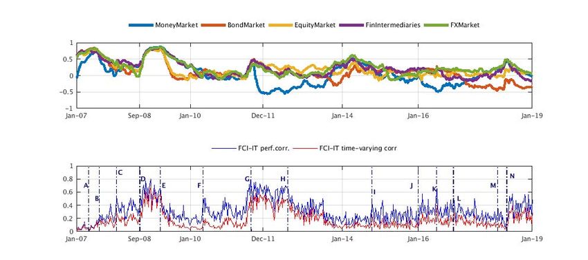
varying, thus enabling us to capture the evolution of systemic risk. The upper panel in Figure 1
shows the average estimated cross-correlations among the five markets selected for the analysis,
while the lower panel reports the Italian FCI computed under both a ‘perfect correlation’ and a
‘normal’ scenario, according to the formula in equation (3).
13
The time-varying correlations ρ , are estimated recursively following an exponentially-weighted moving average
model with a decay lambda-factor equal to 0.93.
14
The evolutions of the raw stress indicators, as well as their ECDF, are reported in Figures 1 and 2 in the Appendix.
Unit-free stress variables and market sub-indices of financial stress are, respectively, reported in Figures 3 and 4 in the
Appendix. Unit-free stress indicators are obtained according to formula (2) in Section 3, with 0 representing a situation
of minimum risk and 1 of maximum risk. Comparable indicators are combined by taking a simple arithmetic average,
thereby obtaining the five market sub-indices of financial stress.
11Figure 1
Average time-varying correlations
and the Italian Financial Condition Index (1) (2)
Source: Thomson Reuters Datastream and authors’ calculations.
(1) The figure shows the average estimated time-varying correlation between each market segment and the remaining four
considered; (2) The indicator’s range of variation is [0,1], where 0 represents a state of minimum systemic risk while 1 is of
maximum risk; (A) First signs in the US of financial losses due to exposure in the subprime mortgage market; (B) BNP Paribas halts
redemptions on three of its Investment Funds; (C) The US Federal Reserve cuts rates by three quarters of a percentage point; (D)
Lehman Brothers’ default; (E) G20 finance ministers and central banks’ pre-summit in London; (F) Greek sovereign debt crisis; (G)
Concerns over sovereign debt sustainability spread to Italy and Spain; (H) Draghi announces that ‘The ECB is ready to do whatever it
takes’; (I) Uncertainty about the Greek political and financial situation; (J) Heightened uncertainty over global growth prospects and
sharp correction of share prices; (K) UK Referendum on Brexit; (L) Italian constitutional referendum; (M) VIX turmoil; (N) New
government in Italy following March general election.
As expected, the two indicators almost overlap when cross-correlations are high. The FCI for the
Italian economy started increasing in March 2007, when the first signs of the forthcoming wave of
financial losses due to exposure to the US subprime mortgage market appeared (point A in Figure
1). Subsequently, the tensions in financial markets accumulated gradually (point B in Figure 1)
leading to the outbreak of the crisis in September 2008 when Lehman Brothers collapsed (point D
in Figure 1). The panic and uncertainty which followed the event pushed the indicator up further,
until it reached its historical peak of about 0.7 in December 2008. Following the extraordinary
monetary policy measures undertaken by central banks in the aftermath of the crisis, the indicator
slowly declined (point E in Figure 1).15 The intensification of the Greek sovereign debt crisis in
spring 2010, and its propagation to other Eurozone countries, led to an uptick in systemic risk (point
F in Figure 1); the announcement of the Securities Market Programme on May 10 marks, amid
15
The significant drop in mid-March 2009 coincides with the G20 meeting when finance ministers and central banks
decided to implement a large global stimulus package and to propose new regulatory measures to repair and strengthen
the financial system.
12some volatility, a decline in the indicator until the beginning of summer 2011 when a severe
deterioration in global financial markets led to a gradual increase in systemic risk.16 The Italian
sovereign debt crisis, which started later in the summer (August 2011), is well identified by the
dynamics of our metric (point G in Figure 1). The appointment of a new government in November
2011 contributed relatively little to ease financial conditions. The indicator in fact continued to stay
at high levels, despite some short-lived decreases following the big take-up by Italian banks of the
3-year LTROs in December 2011 and February 2012. The statement by the ECB President, Mr.
Mario Draghi, in July 2012 (‘Within our mandate, the ECB is ready to do whatever it takes to
preserve the euro. And believe me, it will be enough’; point H in Figure 1) helped to mitigate market
concerns about the euro’s irreversibility and gradually pushed the indicator down for a prolonged
period. Systemic risk increased slightly at the end of 2015, following the resolution of four banks in
crisis under special administration, and in the early months of 2016 when heightened uncertainty
over global growth prospects led to a sharp correction of share prices and increased volatility on
capital markets around the world (point J in Figure 1). The decline in prices was especially marked
for banks’ securities; in Italy, banks’ stocks valuations were also dampened by the large volume of
non-performing loans and by investors’ uncertainty about the outcome of a few scheduled rights
issues. The volatility which followed the outcome of the UK Referendum on leaving the European
Union in June 2016 is also well captured (point K in Figure 1). The release of the EBA 2016 stress
test results at the end of July did not significantly alter the risk outlook for the Italian financial
markets; similarly the Italian referendum on constitutional reforms in late 2016 also had temporary
small effects (point L in Figure 1). Similarly, the sharp correction in stock markets in late January
and early February 2018 led to a negligible increase in the indicator (point M in Figure 1). By
contrast, the market tensions which began in mid-May 2018 were reflected in the FCI’s dynamics,
with the indicator jumping from 0.08 at the beginning of May to 0.32 at the end of the same month
(point N in Figure 1); these levels are lower than those seen during the sovereign debt crisis of
2011-12. Since then the indicator has stabilized at relatively higher levels in comparison to the
previous part of the year.
Taking the difference between the indicators obtained in ‘normal’ situations and the ‘perfect
correlation’ allows us to disentangle the extent to which higher (lower) portfolio diversification
16
The renewed tensions were due primarily to increased concerns regarding the global economic outlook, the
sustainability of public finances in the United States and the possible spread of the European sovereign debt crisis to
Spain and Italy. In those days the US government debt was approaching its ceiling. The Congress and the US
Administration reached a last-minute agreement on a fiscal consolidation plan. In the same period, there was
widespread concern that rating agencies would downgrade and/or assign a negative outlook to the US federal
government.
13contributes to reduce (increase) systemic risk. The closer markets co-move – which can
alternatively happen in periods of calm or distress – the lower the level of portfolio diversification
and the more limited the role of cross-correlations to systemic risk reduction (Figure 2). 17
Figure 2
Decomposition of the Italian FCI
Source: Thomson Reuters Datastream and authors’ calculations.
Following the collapse of Lehman Brothers in September 2008, systemic risk built up especially in
the money market, the financial intermediaries and the foreign exchange segments, which provided
the largest contribution to the FCI in Italy; there was also significant distress in the equity and bond
markets, although their contribution was relatively less pronounced. When the sovereign debt crisis
erupted, the bond and financial intermediaries’ sectors accounted for most of the systemic distress;
the equity and foreign exchange segments followed, while the money market accounted for
relatively less. Following the tensions in mid-May 2018, systemic risk was especially marked in the
bond market, followed by the financial intermediaries’ segments.
Correlation over the whole sample of our index with the euro-area CISS amounts to 0.69. This
relatively high value is not surprising as market-based FCIs are in general very much correlated.
According to the literature, increasing financial integration and openness over the past decade has
led to the emergence of a ‘global financial cycle’ which is characterized by the co-movement of
17
The shaded areas are obtained by the following procedure: 1) squaring the five market sub-indices , , for i=1…5 and
t=1…T; 2) computing, for each t, , / , with i=1…5 and t=1…T; (3) multiplying, for each point in time, the matrix
obtained in step 2 with the FCI under the perfect correlation hypothesis. The sum of these five components equals the
FCI under the perfect correlation scenario.
14cross-border flows and more aligned risky assets prices across different economies (Rey, 2015;
ECB, 2018). This is especially true when financial markets are also exposed to the same monetary
policy which could make some raw indicators move very tightly, especially in those segments
crucial for the transmission mechanism (e.g. money markets). In the light of these considerations,
one may argue that the euro-area CISS would be sufficient to infer financial stability risks
accumulating in Italy. We challenge this view. First, we see merit in having an in-house built metric
of systemic distress which can allow a real-time monitoring of financial stability risks for the Italian
economy. Second, this measure could integrate the information contained in the Risk Dashboard for
the Italian economy, thus enhancing the toolkit available for financial stability risks’ monitoring.
Third, indicators of general systemic stress have been included by the ESRB among the metrics to
analyze during the release phase of the Countercyclical Capital Buffer (ESRB, 2014). In the next
section we show that the proposed indicator has its own value with respect to other metrics; it also
convincingly describes the interaction between the financial sector and the real economy.
5. Feedback loop between the Italian financial sector and the real sector: a TVAR approach
Activity in the real economy could be severely endangered when financial conditions deteriorate.
Systemic risk could be a cause of major concern when its materialization unfolds into large
economic shocks, which affect the distribution of real economic growth.
In this section, we attempt to integrate the so-called ‘vertical view’ (ECB, 2011) into our analysis
assessing whether the proposed measure is able to give significant and consistent information about
the evolution of macroeconomic variables when financial conditions change. To take into account
the non-linear mechanisms that link financial markets to the real economy we estimate a very
simple bivariate TVAR model, which allows for the possibility of regime switching any time an
observable variable crosses a certain threshold.18 The main goal of this empirical exercise is to test
the capacity of the proposed metric to capture the state-dependent adverse feedback loop between
the financial sector and the real economy during periods of financial instability. The FCI
performance is then evaluated against two alternative indicators of systemic stress for the Italian
financial markets, namely the euro-area CISS and the Italian CLIFS (Country Level Index of
Financial Stress), which exhibit a relatively high level of correlation with the Italian FCI
(respectively 0.69 and 0.64). As we will show next in the section regarding the IRFs analysis and
forecasting exercise, there is no clear evidence of superior behaviour. However, the comparison
18
In our application, the TVAR model provides a method to split the sample into different regimes. Within each regime,
a linear VAR model is then estimated.
15may suffer from the fact that the estimation period includes a global deep financial crisis which may
drive results in the same direction, thus providing a pretty similar performance.
In this framework, the Italian FCI and the monthly growth in Italian gross domestic product are
taken as endogenous variables to allow for flexibility in model parameters through a regime
switching behavior.19 In this simple framework, only two regimes exist (high-stress vs. low-stress)
and one threshold is estimated.20 The conjecture underlying the selected model is that financial
shocks have a different role in the two regimes, with a stronger impact on output when financial
conditions are tighter (i.e. during high-stress regimes). The basic specification is the following:
for (4a)
for (4b)
Where high and low indicate, respectively, high- and low-stress regimes. In the above set-up, the
vector , contains the two endogenous variables (i.e. the monthly average FCI
and the monthly growth in GDP), and are respectively the intercept and the matrix of the
slope coefficients for lags j = 1, 2, is the vector of regression errors for states s= high, low, with
~ 0, ). The threshold variable is denoted by , with d representing the delay
parameter and the threshold parameter; in our application, the FCI is the threshold variable whose
dynamics determine regime switch across the two regimes.
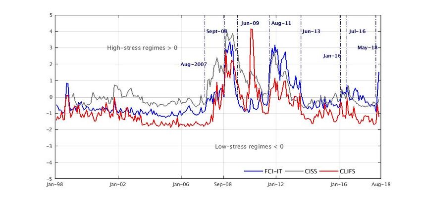
The thresholds deriving from the estimation of the TVAR model in (4a-4b) are shown in Figure 3
(together with the respective indicator computed on a monthly basis), with values equal to about
0.14 (euro-area CISS), 0.15 (Italian FCI) and 0.18 (Italian CLIFS). Figure 4 plots the difference
between the financial condition indicator and the estimated threshold (normalized by standard
deviation); positive (negative) values are classified as high-stress (low-stress) regimes.
19
The model is estimated over the period January 1998 to June 2018. It is worth recalling that the CISS indicator has
been available since January 1999. The monthly observations for Italian GDP are estimated taking into account the
evolution of the Italian industrial production index.
20
A more exhaustive model could certainly fit the data better and provide a more reliable estimate of the economic
impact of financial distress, but this is beyond the scope of this analysis.
16Figure 3
Estimated thresholds
Source: Thomson Reuters Datastream and authors’ calculations.
Figure 4
High-stress vs. low-stress regimes
Source: Thomson Reuters Datastream and authors’ calculations.
Visual inspection indicates that overall our index behaves quite similarly to the other two metrics in
signalling high-stress periods. Unlike the other two metrics, the period spring/summer 2010 is not
classified as high stress; during the first phase of the euro-area sovereign debt crisis Italy was in fact
only marginally affected. More importantly, our FCI spots episodes of financial distress, which are
disregarded by the other two. For instance, our indicator (and the euro-area CISS) would consider
the first half of 2016, as well as the end of the year, as ‘high stress’ periods reflecting the volatility
17which followed the global stock market sell-off (February), the UK vote on Brexit (June) and the
fall of the Government in December. More importantly, during the recent tensions in mid-May, the
Italian FCI enters a ‘high-stress mode’ while the other two remain in a safe area.
To explore more in depth the hypothesis that financial shocks play a different role in the two
regimes, we apply Impulse-Response-Functions (IRFs) analysis. Figure 5 shows the estimated
impact of systemic stress in terms of real economic activity. In particular, we focus on the responses
of Italian GDP (right column) to a one-standard-deviation shock in financial conditions (left
column); the size of the shock changes across regimes. Low- and high-stress periods are,
respectively, shown in the upper and lower panel. For each regime, we report median responses and
68 per cent confidence bands. This exercise is replicated over the three systemic risk indicators
considered.
The use of the newly constructed FCI for the Italian economy produces the following results: during
periods of low stress, the effects of financial shocks on gross domestic product are negligible; in
contrast, output would drop during high-stress periods with a cumulated loss of about 0.9 per cent
on an annual basis. In contrast, a one-standard-deviation shock in the euro-area CISS would make
Italian GDP decline in both states, with output falling to a larger extent during high-stress regimes
(-0.8 versus -0.3 per cent on an annual basis, respectively for the high- and low-stress regime). The
Italian CLIFS instead produces counterintuitive results, as output would remain flat during high-
stress regimes and decline during low-stress periods. These findings suggest that the CLIFS metric
does not capture in a convincing way the adverse impact that states of financial instability could
have in terms of economic activity for the Italian economy. We therefore restrict the ‘horse race’
between the FCI-IT and the euro area CISS.
One striking feature emerges from the above analysis: for both indicators the drop in output is more
pronounced during crisis times. The diverse patterns and responses during low- and high-stress
regimes can be partly attributed to the fact that the standard deviation of the shocks is, for both
indicators, slightly larger during high-stress regimes (Figure 5, right panel).
18Figure 5
Impulse Response Functions Analysis - One standard deviation shock
GDP growth Financial conditions index
Italian FCI
Euro-area CISS
Italian CLIFS
In order to focus on the role of the transmission mechanism only, we follow Alessandri and
Mumtaz (2017) and compute IRFs when shocks are normalized in both regimes to the same
magnitude (0.2 units). The results are shown in Figure 7 in the Appendix. For both financial
19condition indicators, the drop in GDP is still much larger than the one observed during low-stress
periods thus indicating that the transmission mechanism which characterizes the regime also plays a
role. However, confidence bands are wider thus providing an indication that the impact of the
transmission mechanism is estimated with relatively less precision than the shock itself.
A number of standard diagnostics have been computed over the entire period to select the best
fitting variable to estimate the model in 4(a)-4(b); for our purpose, we have focused on equation 2,
which delivers the estimated impact of financial conditions on GDP growth. The results show that
the FCI-IT indicator performs relatively better during high-stress regimes. The RMSEs for equation
2 indicates that the specification including the FCI-IT tends to be marginally more accurate than the
one using the euro-area CISS during high-stress regimes; it is instead slightly less precise in the
case of low-stress regimes.
FCI CISS
Low Stress High Stress Low Stress High Stress
R-squared
Equation1 0.37 0.61 0.32 0.86
Equation2 0.38 0.16 0.27 0.25
R-adjusted
Equation1 0.35 0.58 0.30 0.85
Equation2 0.37 0.09 0.24 0.21
RMSE
Equation1 0.03 0.04 0.03 0.04
Equation2 0.74 0.41 0.63 0.64
As a final step, we perform a forecasting exercise to compare the out-of-sample forecasting
accuracy of the two composite indicators considered (i.e. IT-FCI and euro-area CISS). The model is
estimated recursively over an expanding data window, which starts from January 1998 until
December 2013.21 We examine horizons of one, three, six and twelve months. The first columns of
Table 3 show the average root mean square errors (RMSE) produced by the model using the two
indicators over the evaluation period which runs from January 2014 to June 2018; the following
columns show the same statistics computed over different evaluation periods.22 The results suggest
that the proposed indicator does not perform better than the euro-area CISS in forecasting Italian
21
The model using the euro-area CISS is estimated from January 1999, which is the first date of observation.
22
Computing point forecasts is more complicated in light of the non-linear nature of our model. Following Terasvirta
(2005), the (t+1) forecast is determined given the regime prevailing at point t. From (t+2) on, the forecast is obtained
determining endogenously whether the regime is low/high-stress. In this respect, the procedure runs as follows: 1) the
(with j=1…11) is shocked with ϵi drawn from a N(0,Σst), s=low/high-stress regime and i =1…n); 2) for
each i, the TVAR model is estimated given the prevailing regime and the forecasts obtained in the previous periods for
lagged variables; 3) the forecasts obtained over the n-draws are then averaged to obtain a point forecast for period t.
20GDP; the ratio of the average RMSEs is always around 1 and there is no clear improvement from
estimating the model over longer evaluation periods. A word of caution is, however, necessary
when interpreting these findings. The results may suffer from the low number of observations in the
high-stress scenario (25 and 42 per cent respectively for the Italian FCI and the euro-area CISS).
These observations are more frequent after 2007; therefore, the estimates may be affected by the
dynamics observed during the latest global financial crisis. A longer time period would be
preferable to compare the predictive power of both variables. However, due to data limitations – in
particular for the euro-area CISS – it is not possible to expand the estimation period to include data
points before January 1999.
1998-2013 1998-2014 1998-2015 1998-2016
1M 3M 6M 12M 1M 3M 6M 12M 1M 3M 6M 12M 1M 3M 6M 12M
IT-FCI (a) 0.30 0.21 0.21 0.21 0.20 0.22 0.23 0.23 0.33 0.22 0.20 0.21 0.24 0.25 0.27 0.22
euro-area CISS (b) 0.31 0.21 0.21 0.21 0.20 0.22 0.23 0.23 0.33 0.24 0.21 0.21 0.24 0.27 0.26 0.22
Ratio (a/b) 0.98 0.98 0.99 1.00 1.03 1.00 0.99 0.99 1.00 0.91 0.95 1.00 1.00 0.94 1.02 0.99
Conclusions
The financial crisis has demonstrated the importance of using an analytical toolkit to analyze and
monitor systemic risk. As a consequence, FCIs have been developed by a number of central banks
and international institutions to support monetary and macroprudential tasks, as well as to monitor
the build-up of risks within the system. We developed a first index of financial conditions for the
Italian economy. It can serve as a useful tool to gauge the state of stability/instability within
financial markets. The most important implications of our index for systemic risk monitoring are
the following: 1) the daily frequency can provide a real-time assessment of stress levels within the
system; 2) the decomposition can give information on how much each financial market contributes
to the build-up of systemic stress at any given point in time thus allowing us to pinpoint accurately
where financial stress is accumulating. Possible extensions for future work could include: i) the
broadening of the framework to incorporate data on both infrastructures and the shadow banking
system so as to get a very comprehensive measure for the whole system; ii) the refinement of the
list of raw indicators by means of statistical techniques (e.g. Area Under the Receiver Operator
Curve - AUROC) and iii) the analysis of the role of cross-sectional links (i.e. contagion risks) in
order to gauge the channels through which financial shocks are amplified.
21APPENDIX: supplementary charts
Figure 1
Raw stress indicators
Source: Thomson Reuters Datastream and authors’ calculations.
Figure 2
Quantile transformation of raw stress indicators
Source: Thomson Reuters Datastream and authors’ calculations.
22Figure 3
Unit-free stress indicators
Source: Thomson Reuters Datastream and authors’ calculations.
Figure 4
Financial stress indicators by market
Source: Thomson Reuters Datastream and authors’ calculations.
23Figure 5
Average time-varying correlations
and the Italian Financial Condition Index (1) (2)
Source: Thomson Reuters Datastream and authors’ calculations.
(1) The figure shows the average estimated time-varying correlation between each market segment and the remaining four
considered; (2) The indicator’s range of variation is [0,1], where 0 represents a state of minimum systemic risk while 1 of maximum
risk; (A) Russian crisis and LTCM default; (B) First signs in the US of financial losses due to exposure in the subprime mortgage
market; (C) BNP Paribas halts redemptions on three of its Investment Funds; (D) The US Federal Reserve cuts rates by three quarters
of a percentage point; (E) Lehman Brothers’ default; (F) G20 finance ministers and central banks’ pre-summit in London; (G) Greek
sovereign debt crisis; (H) Concerns over sovereign debt sustainability spread to Italy and Spain; (I) Draghi announces that ‘The ECB
is ready to do whatever it takes’; (J) Uncertainty about the Greek political and financial situation; (K) Heightened uncertainty over
global growth prospects and sharp correction of share prices; (L) UK Referendum on Brexit; (M) Italian constitutional referendum;
(N) VIX turmoil; (O) New government in Italy following March general election.
Figure 6
Decomposition of the Italian Financial Condition Index
Source: Thomson Reuters Datastream and authors’ calculations.
24Figure 7
Impulse response functions of GDP growth
standardized shock = 0.2
Italian FCI Euro-area CISS
25References
Adrian T, Boyarchenko N. and Giannone D. (2017). ‘Vulnerable Growth’. Federal Reserve Bank of
New York Staff Reports, No. 794.
Bernanke, B. S., Gertler M. and Gilchrist S. (1999). The financial accelerator in a quantitative
business cycle framework. Handbook of Macroeconomics, ed. by J. B. Taylor and M. Woodford,
Vol. 1, chap. 21, pp. 1341 and 1393, Elsevier.
Brave, S. and Butters A., (2012). ‘Diagnosing the Financial System: Financial Conditions and
Financial Stress’. International Journal of Central Banking, Vol. 8, No. 2, 191-239.
Cardarelli R., Elekdag S. and Lall S., (2011). ‘Financial stress and economic contractions’. Journal
of Financial Stability, Vol. 7, No. 2, 78-97.
Duprey, T., Klaus, B. and Peltonen T. (2017). ‘Dating systemic financial stress episodes in the EU
countries’. Journal of Financial Stability, Vol. 32, 30-56.
European Central Bank, (2011). ‘Special feature C: Systemic risk methodologies’. Financial
Stability Review, June, 141-148.
European Central Bank, (2018). ‘The global financial cycle: implications for the global economy
and the euro-area’. ECB Economic Bulletin, Issue 6/2018.
European Systemic Risk Board (2014), Recommendations of the European Systemic Risk Board on
guidance for setting countercyclical buffer rates (ESRB/2014/1)
Giglio, S., Kelly B., and Pruitt S. (2016). ‘Systemic risk and the macroeconomy: An empirical
evaluation’, Journal of Financial Economics, 119, 457–471.
Hakkio, C. S., and W. R. Keeton. 2009. ‘Financial Stress: What Is It, How Can It Be Measured, and
Why Does It Matter?’. Economic Review (Federal Reserve Bank of Kansas City) (Second Quarter):
5-50.
Hatzius J., Hooper P., Mishkin F.S., Schoenholtz L.K., and Watson M.W. (2010). ‘Financial
Conditions Indexes: A Fresh Look after the Financial Crisis’. NBER Working Papers No. 16150.
Hollò, D., Kremer, M. and M. Lo Duca, (2012). ‘CISS - a composite indicator of systemic stress in
the financial system’. Working Paper Series 1426, European Central Bank.
Iachini E. and Nobili S. (2014). ‘An indicator of systemic liquidity risk in the Italian financial
markets’. Banca d’Italia, Questioni di economia e finanza (Occasional Papers), 217.
Illing, M. and Liu Y., (2006). ‘Measuring Financial Stress in a Developed Country: an application
to Canada’. Journal of Financial Stability, Vol. 2., No. 4, 243-265.
Kliesen K. and Smith D. C., (2010). ‘Measuring Financial Market Stress’. Federal Reserve Bank of
St. Louis, Economic Synopses, No. 2, January.
Koop, G. and Korobilis D. (2014). ‘A New Index of Financial Conditions’. European Economic
Review, 71, 101-116.
Matheson, T. D. (2012). ‘Financial conditions indexes for the United States and euro area’.
Economics Letters, 115(3), 441-446.
Patel, S. and Sarkar A. (1998). ‘Stock Market Crises in Developed and Emerging Markets’.
Financial Analysts Journal, Vol. 54, pp. 50-59.
Rey, H (2015). ‘Dilemma not Trilemma: the global financial cycle and monetary policy
independence’. NBER Working Paper No. 21162.
Terasvirta, T. (2005), ‘Forecasting with Nonlinear Models’, in G. Elliott, C.W.J. Granger and A.
Timmermann (eds.), Handbook of Economic Forecasting, forthcoming.
Venditti, F., Columba F. and Sorrentino A. (2018), ‘A risk dashboard for the Italian economy’.
Banca d’Italia, Questioni di economia e finanza (Occasional Papers), 425.
26You can also read