Self-Supervised Visibility Learning for Novel View Synthesis
←
→
Page content transcription
If your browser does not render page correctly, please read the page content below
Self-Supervised Visibility Learning for Novel View Synthesis

                                                                             Yujiao Shi 1 , Hongdong Li 1 , Xin Yu 2
                                                         1
                                                           Australian National University and ACRV 2 University of Technology Sydney
                                                              yujiao.shi@anu.edu.au, hongdong.li@anu.edu.au, xin.yu@uts.edu.au
arXiv:2103.15407v2 [cs.CV] 4 Apr 2021

                                        Figure 1: Given a few sparse and unstructured input multi-view images, our goal is to synthesize a novel view from a given target camera pose. Our
                                        method estimates target-view depth and source-view visibility in an end-to-end self-supervised manner. Compared with the previous state-of-the-art, such
                                        as Choi et al. [4] and Riegler and Koltun [24], our method produces superior novel view images of higher quality and with finer details, better conform to
                                        the ground-truth.

                                                                     Abstract                                           bility and target-view depth. At last, our network is trained
                                                                                                                        in an end-to-end self-supervised fashion, thus significantly
                                                                                                                        alleviating error accumulation in view synthesis. Experi-
                                           We address the problem of novel view synthesis (NVS)                         mental results demonstrate that our method generates novel
                                        from a few sparse source view images. Conventional image-                       views in higher quality compared to the state-of-the-art.
                                        based rendering methods estimate scene geometry and syn-
                                        thesize novel views in two separate steps. However, erro-
                                        neous geometry estimation will decrease NVS performance                         1. Introduction
                                        as view synthesis highly depends on the quality of estimated
                                        scene geometry. In this paper, we propose an end-to-end                             Suppose after taking a few snapshots of a famous sculp-
                                        NVS framework to eliminate the error propagation issue.                         ture, we wish to look at the sculpture from some other dif-
                                        To be specific, we construct a volume under the target view                     ferent viewpoints. This task would require us to generate
                                        and design a source-view visibility estimation (SVE) module                     novel-view images from the captured ones and is generally
                                        to determine the visibility of the target-view voxels in each                   referred to as “NVS”. However, compared with previous so-
                                        source view. Next, we aggregate the visibility of all source                    lutions, our setting is more challenging, because the num-
                                        views to achieve a consensus volume. Each voxel in the                          ber of available real views is very limited, and the underly-
                                        consensus volume indicates a surface existence probability.                     ing 3D geometry is not available. Moreover, the occlusion
                                        Then, we present a soft ray-casting (SRC) mechanism to find                     along target viewing rays and the visibility of target pixels
                                        the most front surface in the target view (i.e., depth). Specif-                in source views are hard to infer.
                                        ically, our SRC traverses the consensus volume along view-                          Conventional image-based rendering (IBR) methods [4,
                                        ing rays and then estimates a depth probability distribution.                   24, 10, 42, 23] first reconstruct a proxy geometry by a multi-
                                        We then warp and aggregate source view pixels to synthe-                        view stereo (MVS) algorithm [12, 47, 48, 46]. They then
                                        size a novel view based on the estimated source-view visi-                      aggregate source views to generate the new view according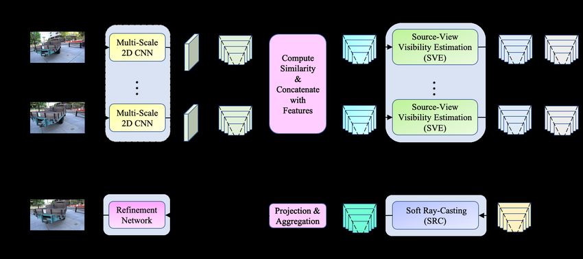
to the estimated geometry. Since the two steps are separated
from each other, their generated image quality is affected by
the accuracy of the reconstructed 3D geometry.
    However, developing an end-to-end framework that
combines geometry estimation and image synthesis is non-
trivial. It requires addressing the following challenges.
First, estimating target view depth by an MVS method will
be no longer suitable for end-to-end training because they
need to infer depth maps for all source views. It is time-
and memory-consuming. Second, when source view depths
                                                                    Figure 2: Given a set of unstructured and disordered source views, we aim
are not available, the visibility of target pixels in each source
                                                                    to synthesize a new view from a position not in the original set. For a
view is hard to infer. A naive aggregation of warped input          3D point lies in a target viewing ray, when its projected pixels on source
images would cause severe image ghosting artifacts.                 view images are consistent with each other, it is of high probability that a
    To tackle the above challenges, we propose to estimate          surface exists at the corresponding location. The color of this surface can
                                                                    be computed as a visibility-aware combination of source view pixel colors.
target-view depth and source-view visibility directly from
source view images, without estimating depths for source
views. Specifically, we construct a volume under the target
                                                                    rendering problem as a color reconstruction without explicit
view camera frustum. For each voxel in this volume, when
                                                                    3D geometry modelling. Penner and Zhang [23] propose
its projected pixel in a source view is similar to the projected
                                                                    a soft 3D reconstruction model that maintains continuity
pixels in other source views, it is likely that the voxel is
                                                                    across views and handles depth uncertainty.
visible in this source view. Motivated by this, we design
                                                                        Learning-based methods. Recently, learning-based ap-
a source-view visibility estimation module (SVE). For each
                                                                    proaches have demonstrated their powerful capability of
source view, our SVE takes the warped source view features
                                                                    rendering new views. Several works have been proposed to
as input, compares their similarity with other source views,
                                                                    train a neural network that learns geometry implicitly and
and outputs visibility of the voxels in this source view.
                                                                    then synthesizes new views [53, 39, 20, 22, 6, 51]. Most
    Then, we aggregate the estimated visibility of the vox-
                                                                    of those methods can synthesize arbitrarily new views from
els in all source views, obtaining a consensus volume. The
                                                                    limited input views. However, their performance is limited
value in each voxel denotes a surface existence probability.
                                                                    due to the lack of built-in knowledge of scene geometry.
Next, we design a soft ray-casting (SRC) mechanism that
                                                                        Scene representations. Some end-to-end novel view
traverses through the consensus volume along viewing rays
                                                                    synthesis methods model geometry by introducing spe-
and finds the most front surfaces (i.e., depth). Since we do
                                                                    cific scene representations, such as multi-plane images
not have ground truth target-view depth as supervision, our
                                                                    (MPI) [52, 18, 38, 43, 8] and layered depth images
SRC outputs a depth probability instead of a depth map to
                                                                    (LDI) [29, 44, 34, 44]. MPI represents a scene by a set
model uncertainty.
                                                                    of front-parallel multi-plane images, and then a novel view
    Using the estimated target-view depth and source-view
                                                                    image is rendered from it. Similarly, LDI depicts a scene in
visibility, we warp and aggregate source view pixels to gen-
                                                                    a layered-depth manner.
erate the novel view. Since the 3D data acquisition is ex-
                                                                        Deep networks have also been used as implicit functions
pensive to achieve in practice, we do not have any explicit
                                                                    to represent a specific scene by encapsulating both geom-
supervision on the depth or visibility. Their training signals
                                                                    etry and appearance from 2D observations [19, 49, 37, 21,
are provided implicitly by the final image synthesis error.
                                                                    36, 41]. Those neural scene representations are differen-
We then employ a refinement network to further reduce ar-
                                                                    tiable and theoretically able to remember all the details of
tifacts and synthesize realistic images. To tolerate the visi-
                                                                    a specific scene. Thus, they can be used to render high-
bility estimation error, we feed our refinement network the
                                                                    quality images. However, since these neural representations
aggregated images along with warped source view images.
                                                                    are used to depict specific scenes, models trained with them
                                                                    are not suitable to synthesize new views from unseen data.
2. Related Work
                                                                        Image-based rendering. Image-based rendering tech-
   Traditional approaches. The study of NVS has a                   niques incorporate geometry knowledge for novel view syn-
long history in the field of computer vision and graph-             thesis. They project input images to a target view by an es-
ics [9, 15, 28, 5]. It has important applications in robot navi-    timated geometry and blend the re-projected images [4, 24,
gation, film industry, and augmented/virtual reality [31, 33,       10, 42, 23]. Thus, they can synthesize free-viewpoint im-
32, 30, 11]. Buehler et al. [2] define an unstructured Lu-          ages and generalize to unseen data. However, as geometry
migraph and introduce the desirable properties for image-           estimation and novel view synthesis are two separate steps,
based rendering. Fitzgibbon et al. [7] solve the image-based        these techniques usually produce artifacts when inaccurate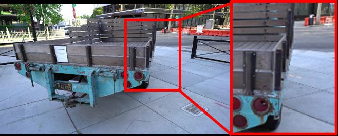
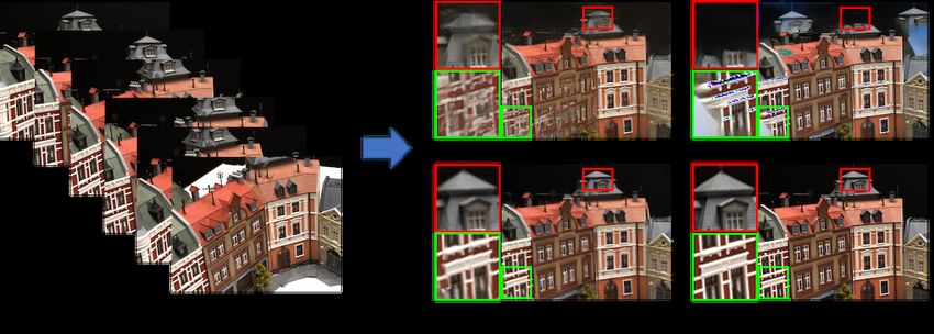
Figure 3: An overall illustration of the proposed framework. We first extract multi-scale features (Phase I) from source images and warp them to the
target view. We then design a source-view visibility estimation (SVE) module (Phase II) to estimate the visibility of target voxels in each source view. By
aggregating visibility features from all source views, we construct a consensus volume to represent surface existence at different voxels. Next, we design an
LSTM-based soft ray-casting (SRC) mechanism (Phase III) to render the depth probability from the consensus volume. By using the estimated source-view
visibility and target-view depth, we warp and aggregate source view images. We finally apply a refinement network (Phase IV) to further reduce artifacts in
the aggregated images and synthesize realistic novel views.

geometry or occlusions occur. Choi et al. [4] estimate a                             We assume a uniform prior on the target view depth, and
depth map in the target view by warping source view prob-                         reformulate Eq. (1) as a probability conditioned on depth d:
ability distributions computed by DeepMVS [12]. To tol-                                                                  dmax
erate inaccurate depths, aggregated images as well as orig-
                                                                                                                         X
                                                                                                 I t∗ = argmax                   p I t |d p (d)

inal patches extracted from source view images are fed to                                                     It        d=dmin
their proposed refinement network. Riegler and Koltun [24]                                                                                                 (2)
                                                                                                          dmax
                                                                                                          X
                                                                                                                                          t
leverage COLMAP [26, 27] to reconstruct 3D meshes from

                                                                                                     =                 argmax p I |d               p(d),
a whole sequence of input images and obtain target view                                                  d=dmin          It

depths using the estimated geometry.
                                                                                  where dmin and dmax are statistical minimum and maximum
3. Problem Statement                                                              depths of a target view respectively. As the source view
                                                                                  images are given, we omit them in this equation.
     Our goal is to synthesize a novel view I t , given target                       Following conventional methods, we compute the target
camera parameters K t , Rt , T t , from a set of input images,                    view color I t with the highest probability given depth d as
Iis , i = 1, 2, ..., N . We assume there is sufficient overlap                    a visibility-aware combination of source view colors:
between the source views such that correspondences can be                                                             N
established. We estimate source view camera intrinsic and                                                           X
                                                                                                    argmax p I t |d =   wid Cdi ,                          (3)
extrinsic by a well-established structure-from-motion (SfM)                                              It                         i=1
pipeline, e.g.COLMAP [26]. Fig. 2 illustrates the situation.
Mathematically, we formulate this problem as:                                     where Cdi ∈ RH×W ×3 is a collection of re-projected tar-
                                                                                  get pixels in source view i by inverse warping [16], wid ∈
               I t∗ = argmax p I t |I1s , I2s , ..., IN
                                                      s
                                                          ,            (1)        RH×W is the blending weight of source view i, and it is
                           It
                                                                                  computed from the visibility of target pixels in each source
where p(·) is a probability function.
                                                                                  view:
    Due to the expensive accessibility of 3D data (e.g.,                                                      X  N
depths) and a limited number of input views, it is hard to                                         wid = exp Vid /   exp Vid ,                             (4)
compute accurate 3D geometry from input source views.                                                                         i=1

Therefore, our intuition is to develop an end-to-end frame-                       where Vid ∈ RH×W is the visibility of target pixels in
work that combines geometry estimation and image synthe-                          source view i given the target-view depth d.
sis, to eliminate the error propagation issue. We achieve                            In the next section, we will provide technical details on
this goal by estimating target-view depth and source-view                         how to estimate the source-view visibility Vid and target-
visibility for target pixels directly under the target view.                      view depth probability distribution p(d).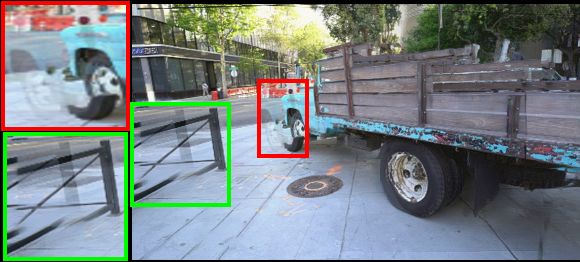
4. The Proposed Framework
   We aim to construct an end-to-end framework for novel
view synthesis from a few sparse input images. By doing so,
inaccurately-estimated geometry can be corrected by image
synthesis error during training. We achieve this goal by esti-
mating target-view depth and source-view visibility directly
under the target view. Fig. 3 depicts the proposed pipeline.
   Start from a blank volume in the target-view camera frus-
tum. Our goal is to select pixels from source-view images           Figure 4: Illustration of our soft ray-casting mechanism. Our SRC tra-
to fill in the voxels of this volume. After that, we can ren-       verses through the surface probability curve along target viewing rays from
                                                                    near to far, increases the depth probability of the first opaque element, and
der the target view image from this colored volume. In this         decreases depth probabilities of later elements no matter they are opaque
process, the visibility of the voxels in each source view, and      or not.
the target-view depth, are two of the most crucial issues.

4.1. A multi-scale 2D CNN to extract features                       depth dimension. Our SVE module takes into account self-
                                                                    information (Fdi ), local information (Sdi ) and global infor-
    When a voxel of this volume is visible in a source view,                 PN
                                                                    mation ( i=1 Sdi /N ) to determine the visibility of the vox-
its projected pixel in this source view should be similar to
                                                                    els in each source view. Mathematically, we express it as:
the projected pixels in other source views. This is the under-
lying idea for the source-view visibility estimation. How-                                        "                 N
                                                                                                                    X
                                                                                                                                   #                 !
ever, the pixel-wise similarity measure is not suitable for            Vid , Bdi , statedf   =f       Fdi , Sdi ,         Sdi /N       , statefd−1       ,   (6)
textureless and reflective regions. Hence, we propose to ex-                                                        i=1

tract high-level features from source view images for the           where [·] is a concatenation operation, Vid ∈ RH×W is
visibility estimation by a 2D CNN.                                  the estimated visibility for target-view voxels at depth d in
    Our 2D CNN includes a set of dilation convolutional lay-        source view i, Bdi ∈ RH×W ×8 is the associated visibility
ers with dilation rates as 1, 2, 3, 4 respectively. Its output is   feature, f (·) denotes the proposed SVE module, stated−1 f
a concatenation of extracted multi-scale features. This de-         is the past memory of our SVE module before depth d and
sign is to increase the receptive field of extracted features       statedf is the updated memory at depth d.
and retain low-level detailed information [45], thus increas-
ing discriminativeness for source view pixels.                      4.3. Soft ray-casting (SRC) mechanism
    Denote Fi ∈ RH×W ×D×C as the warped features of
                                                                       By aggregating visibility from all source views, we ob-
source view i, where D is the sampled depth plane number
                                                                    tain a surface existence probability for each voxel in the tar-
in the target view. For target-view voxels at depth d, we
                                                                    get view. As shown in Fig. 4, the surface probability curve
compute the similarity between corresponding features in
                                                                    along a target viewing ray might be multi-modal, where
source view i and other source views as:
                                                                    a smaller peak indicates that a surface is visible by fewer
                     N
                     X                                            source views and a larger peak suggests that its correspond-
            Sdi =              Sim Fdi , Fdj /(N − 1),        (5)   ing surface is visible by a large number of source views.
                    j=1,j6=i
                                                                       To increase the representative ability, we aggregate the
                                                                    visibility features, instead of visibility, of source views to
where Sim(·, ·) is a similarity measure between its two in-
                                                                    compute a consensus volume:
puts, and we adopt cross-correlation in this paper.
                                                                                                          N
                                                                                                          X
4.2. Source-view visibility estimation (SVE) module                                               C=            Bi /N,                                       (7)
                                                                                                          i=1
    In theory, deep networks are able to learn viewpoint in-
variant features. However, we do not have any explicit su-          where C ∈ RH×W ×D×8 is the obtained consensus volume.
pervision on the warped source-view features. The compu-               Then, we design a soft ray-casting (SRC) mechanism to
tation of source-view visibility for the voxels is too com-         render the target view depth from the consensus volume.
plex to be modeled by Eq. (5). Hence, we propose to learn           Our SRC is implemented in the form of an LSTM layer.
a source-view visibility estimation (SVE) module to predict         Similar to our SVE module, the LSTM layer is to encode
the visibility of the voxels in each source view.                   sequential relationship along the depth dimension.
    Our SVE module is designed as an encoder-decoder ar-               The LSTM layer traverses though the consensus volume
chitecture with an LSTM layer at each stage. The LSTM               along target viewing rays from near to far. When meeting
layer is adopted to encode sequential information along the         the most front surface, it outputs a large depth probability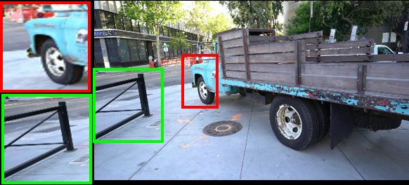
value for the corresponding voxel. For the later voxels, the                  5. Experiments
LSTM layer sets their probability values to zero. Denote
the LSTM cell as r(·). At each depth d, it takes as input the                     Dataset and evaluation metric. We conduct exper-
current consensus feature C d and its past memory staterd−1 ,                 iments on two datasets, Tanks and Temples [14], and
and outputs the depth probability p(d) along with the up-                     DTU [1]. Camera movements in the two datasets include
                                                                              both rotations and translations.
dated memory statedr :
                                                                                  On the Tanks and Temples, we use the training and
                statedr , p(d) = r(C d , stated−1
                                              r   ).                    (8)   testing split provided by Riegler and Koltun [24]. In this
                                                                              dataset, 17 out of 21 scenes are selected out as the train-
4.4. Refinement network                                                       ing set. The remaining four scenes, Truck, Train, M60, and
                                                                              Playground, are employed as the testing set. We apply the
    Using the estimated source-view visibility and target-                    leave-one-out strategy for training, namely, designating one
view depth probability, we aggregate the source images and                    of the images as target image and selecting its nearby N
obtain I t∗ by Eq. (2). We then employ a refinement network                   images as input source images. For testing, different from
to further reduce artifacts on the aggregated image.                          Riegler and Koltun [24] which uses whole sequences as in-
    Our refinement network is designed in an encoder-                         put, we select N nearby input images for each target view.
decoder architecture with convolutional layers. To tolerate                       For the DTU dataset, it is employed to further demon-
errors caused by the visibility estimation block, the encoder                 strate the generalization ability of trained models. We do
in our refinement network is in two branches: one for the                     not train on this dataset and use the validation set provided
                     t∗
aggregatedPDimage I and another for a warped source view                      by Yao et al. [47]. The validation set includes 18 scenes.
Iiwarp = d=1 Cdi p(d). Its outputs are a synthesized target                   Each of the scenes contains 49 images. We apply the same
view image Iˆit along with a confidence map mi :                              leave-one-out strategy as on the Tanks and Temples dataset.
                                              warp                                Following recent NVS works [4, 24, 17, 8], we adopt the
               Iˆit , mi = Refinement(I t∗ , Ii ).                      (9)
                                                                              commonly used SSIM, PSNR and LPIPS [50] for quality
The final output of our refinement network is computed as:                    evaluation on synthesized images.
                                   N
                                                                                  Implementation details. For the Tanks and Temples,
                        Iet =
                                   X
                                         mi Iˆit .                     (10)   we experiment on image resolution of 256 × 448. For the
                                   i=1                                        DTU dataset, the input image resolution is 256 × 320. We
                                                                              use a TITAN V with 12GB memory to train and evaluate
4.5. Training objective                                                       our models. We train 10 epochs on the Tanks and Tem-
   We employ the GAN training scheme to train our frame-                      ples dataset with a batch size of 1. It takes 20 hours for
work. For brevity, we omit the adversarial loss in this pa-                   training using 6 input images, and 0.35s per image (av-
per. Interested readers are referred to Isola et al. [13]. For                erage) for evaluation. We apply inverse depth sampling
the target image supervision, we adopt the perceptual loss                    strategy with depth plane number D = 48. For outdoor
of Chen and Koltun [3]:                                                       scenes, i.e., the Tanks and Temples, we set dmin = 0.5m and
                               X                                              dmax = 100m. For constrained scenes, i.e., the DTU dataset,
    Lper = Iet − I t       +        λl φl (Iet ) − φl (I t )       ,   (11)   we employ the minimum (425mm) and maximum (937mm)
                       1                                       1
                               l
                                                                              depth in the whole dataset. The source code of this paper
where φ(·) indicates the outputs of a set of layers from a                    is available at https://github.com/shiyujiao/
pretrained VGG-19 [35], and k·k1 is the L1 distance. The                      SVNVS.git.
settings for coefficients λl are the same as Zhou et al. [52].
                                                                              5.1. Comparison with the state-of-the-art
   Self-supervised training signal for our SRC and SVE.
Generally, it is difficult for our SRC to decide which is the                    We first compare with two recent and representative IBR
most front surface in a viewing ray, especially when the                      methods, Extreme View Synthesis (EVS) [4] and Free View
surface probability curve is multi-modal. We expect this                      Synthesis (FVS) [24], with six views as input. We present
soft determination can be learned statistically from training.                the quantitative evaluation in the first three rows of Tab. 1.
Particularly, when the estimated depth is incorrect, the color                Qualitative comparisons on the Tanks and Temples are pre-
of warped pixels from source-view images will deviate from                    sented in Fig. 5.
the ground truth target view color. This signal would pun-                       Both EVS and FVS first estimate depth maps for source
ish the LSTM and helps it to make the right decisions. The                    views. In their methods, the visibility of target pixels in
same self-supervised training scheme is applied to our SVE                    source views is computed by a photo-consistency check
module. We illustrate the estimated depth for a target pixel                  between source and target view depths. EVS aggregates
in Fig. 4, and an example of the visibility-aware aggregated                  source views simply based on the source-target camera dis-
image in Fig. 7.                                                              tance. Their aggregation weights do not have the ability to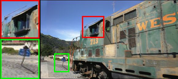
(a) EVS [4]                           (b) FVS [24]                            (c) Ours                           (d) Ground Truth
Figure 5: Qualitative visualization of generated results on the Tanks and Temples dataset with six views as input. The four examples are from scene Truck,
Train, M60, Playground respectively.

Table 1: Quantitative comparison with the state-of-the-art. Here, “Whole” denotes using the whole sequence as input; “*” indicates that results are from
Zhang et al. [49]; and “† ” represents that results are from Riegler and Koltun [24].
             Input                                  Tanks and Temples
                                                                                                       DTU
             View         Truck               Train                   M60        Playground
            Number LPIPS↓ SSIM↑ PSNR↑ LPIPS↓ SSIM↑ PSNR↑ LPIPS↓ SSIM↑ PSNR↑ LPIPS↓ SSIM↑ PSNR↑ LPIPS↓ SSIM↑ PSNR↑
 EVS[4]        6      0.301    0.588   17.74    0.434    0.434    15.38    0.314   0.585    16.40     0.243   0.702   21.57     0.32    0.645    17.83
 FVS[24]       6      0.318    0.638   15.82    0.447    0.502    13.71    0.486   0.548    11.49     0.417   0.586   14.95     0.47    0.530    10.45
  Ours         6      0.233    0.708   21.33    0.386    0.542    18.81    0.250   0.732    19.20     0.245   0.710   22.12    0.303    0.721    19.20
               2      0.294    0.627   19.20    0.475    0.464    17.44    0.303   0.667    18.14     0.350   0.604   19.98    0.362    0.625    17.54
   Ours        4      0.254    0.682   20.41    0.430    0.495    17.82    0.283   0.698    19.37     0.275   0.663   21.31    0.359    0.646    17.84
               6      0.233    0.708   21.33    0.386    0.542    18.81    0.250   0.732    19.20     0.245   0.710   22.12    0.303    0.721    19.20
NeRF[19] Whole        0.513* 0.747* 20.85* 0.651* 0.635* 16.64* 0.602* 0.702* 16.86* 0.529* 0.765* 21.55*                        –        –        –
FVS[24] Whole          0.11† 0.867† 22.62† 0.22† 0.758† 17.90† 0.29† 0.785† 17.14† 0.16† 0.837† 22.03†                           –        –        –

tolerate visibility error caused by in-accurate depth. Thus,                    eralization ability, we employ the trained models of the
the synthesized images by EVS suffer severe ghosting arti-                      three algorithms to test on the DTU dataset. Quantitative re-
facts, as shown in Fig. 5(a). FVS employs a COLMAP to                           sults are presented in the last column of Tab. 1. Our method
reconstruct the 3D mesh. When input images densely cover                        consistently outperforms the recent state-of-the-art algo-
a scene, the reconstructed geometry is exceptionally good,                      rithms. We present two visualization examples in Fig. 6.
and the synthesized images are of high-quality, as shown                        More qualitative results are provided in the supplementary
in the last row of Tab. 1. However, when the number of                          material.
input images are reduced, i.e., 6, the reconstructed mesh
                                                                                   Different input view number. We further conduct ex-
by COLMAP is of poor quality, and the depth-incorrect re-
                                                                                periments on reducing the number of input views of our
gions in the synthesized images are blurred, as indicated
                                                                                method. Quantitative results are presented in the bottom
in 5(b). In contrast, our method does not rely on the accu-
                                                                                part of Tab. 1. Increasing the input view number improves
racy of estimated source-view depths or reconstructed 3D
                                                                                the quality of synthesized images. This conforms to our
mesh. Instead, we directly recover target-view depth and
                                                                                general intuition that image correspondences can be easily
source-view visibility from input images. Thus, our synthe-
                                                                                established and more disoccluded regions can be observed
sized images show higher quality than the recent state-of-
                                                                                when more input views are available.
the-art.
                                                                                   Comparison with NeRF. For completeness, we present
   Generalization ability. To further demonstrate the gen-                      the performance of NeRF [19] with the whole sequence as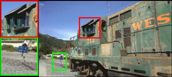
(a) EVS [4]                           (b) FVS [24]                            (c) Ours                         (d) Ground Truth
Figure 6: Qualitative visualization of generated results on the DTU dataset with six views as input. The two examples are from scene scan3 and scan106,
respectively.

input in the penultimate row of Tab. 1. The major differ-                     are presented in the first row of Tab. 2. It can be seen that
ence between NeRF and our method is the different prob-                       the performance drops significantly compared to our whole
lem settings. NeRF is more suitable to view synthesis on a                    pipeline. This indicates that it is hard for the refinement
specific scene with many images as input. When the scene                      network to select visible pixels from source views.
is changed, NeRF needs to be re-trained on the new scene.                         We present a visualization example of our visibility-
In contrast, we expect our network to learn common knowl-                     aware aggregated result in Fig. 7. As shown in Fig. 7(a),
edge from its past observations (training data) and be able                   directly warped source images contain severe ghosting ar-
to apply the learned knowledge to unseen scenes without                       tifacts due to occlusions, i.e., disoccluded regions in tar-
further fine-tuning. Thus, our approach is a better choice                    get view are filled by replicas of visible pixels from a
when the trained model is expected to generalize, and the                     source view. By using the proposed SVE module to esti-
number of input images is small.                                              mate the visibility of source views, our aggregated result,
    Comparison with Szeliski and Golland [40]. We found                       Fig. 7(b), successfully reduces the ghosting artifacts and is
our work shares the same spirit with a classical work [40].                   much more similar to the ground truth image, Fig. 7(c).
Both works construct a virtual camera frustum under the                           Soft ray-casting. We first remove the soft ray-casting
target view and aim to estimate the color and density (depth                  mechanism from our whole pipeline, expressed as “Ours
probability in our work) for each of its elements. Szeliski                   w/o ray-casting”. Instead, we use the surface probability,
and Golland [40] first compute an initial estimation by find-                 i.e., the red curve in Fig. 4, as the depth probability to warp
ing agreement among source views. Next, they project                          and aggregate source views. As indicated by the second row
the estimation to the source views, compute the visibil-                      of Tab. 2, the results are significantly inferior to our whole
ity of source views, and then refine the estimation itera-                    pipeline. Furthermore, we replace the SRC as the conven-
tively. Benefited from learning-based techniques, our ap-                     tional over alpha compositing scheme, denoted as “Ours w
proach encodes the visibility estimation as a single forward                  over compositing”. The results are presented in the third
step (compared to iterative refinement in Szeliski and Gol-                   row of Tab. 2. It can be seen that our SRC is necessary and
land [40]) and can handle more complex scenarios, such as                     cannot be replaced by the over alpha compositing scheme.
textures and reflective regions, as shown in the qualitative                      Both SRC and over alpha compositing are neural render-
visualizations of this paper and supplementary material.                      ers in NVS. Over-compositing uses opacity to handle occlu-
                                                                              sions, while our method does not regress opacity for vox-
5.2. Ablation study
                                                                              els. Our input curve to SRC is obtained by majority voting
    In this section, we conduct experiments to verify the ef-                 from source views. A smaller peak in the curve indicates
fectiveness of each component in the proposed framework.                      that a surface is visible by fewer source views and a larger
    Source-view visibility estimation. We first remove                        peak suggests that a surface is visible by more source views.
the visibility-aware source view aggregation (indicated by                    Due to the fixed weight embedding in over-compositing, the
Eq. (2)) from our framework, denoted as “Ours w/o visi-                       smaller peak at a nearer distance will be ignored while the
bility”. Instead, we feed the warped source images to our                     larger peak will be highlighted. By using LSTM, our SRC
refinement network directly and equally. We expect the                        can be trained to decide which peak is the top-most surface.
refinement network to learn the visibility-aware blending                         Refinement network. We further ablate the refine-
weights for source view images automatically. The results                     ment network. In doing so, we remove the warped source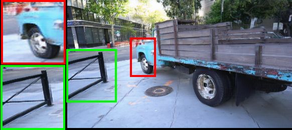
(b) Aggregated Image

                                  (a) Warped Source-View Images in Target View                                 (c) Ground Truth
Figure 7: Qualitative illustration on our visibility-aware aggregation. (a) Warped source images in target view. There are severe ghosting
artifacts due to occlusions. (b) Aggregated image by using our visibility-aware blending weights. (c) Target view ground truth image.

                                           Table 2: Necessity of each module in the proposed framework.
                                                           Tanks and Temples
                                                                                                              DTU
                                 Truck               Train                   M60        Playground
                          LPIPS↓ SSIM↑ PSNR↑ LPIPS↓ SSIM↑ PSNR↑ LPIPS↓ SSIM↑ PSNR↑ LPIPS↓ SSIM↑ PSNR↑ LPIPS↓ SSIM↑ PSNR↑
Ours w/o visibility       0.271   0.660   20.35   0.437   0.482   17.93   0.322   0.656   16.83   0.277   0.665   21.40   0.367   0.641   17.03
Ours w/o ray-casting      0.761   0.643   20.04   0.665   0.487   17.83   0.766   0.654   17.45   0.737   0.649   20.98   0.397   0.649   18.71
Ours w over compositing   0.308   0.695   21.19   0.445   0.531   18.14   0.321   0.709   19.32   0.334   0.689   21.57   0.409   0.684   19.02
Ours w/o warped sources   0.250   0.697   20.89   0.402   0.534   18.58   0.263   0.729   19.31   0.254   0.704   22.51   0.322   0.705   19.65
Ours w/o refinement       0.237   0.675   20.99   0.380   0.533   18.28   0.220   0.717   20.13   0.244   0.689   22.88   0.239   0.765   21.44
Our whole pipeline        0.233   0.708   21.33   0.386   0.542   18.81   0.250   0.732   19.20   0.245   0.710   22.12   0.303   0.721   19.20

view images from the refinement network input, denoted                      be accurately searched. Another limitation of our method is
as “Ours w/o warped sources”. As shown by the results in                    that we have not incorporated temporal consistency into our
Tab. 2, there is only a small performance drop compared to                  method when synthesizing a sequence of new views. There
our whole pipeline. This indicates that our visibility-aware                might be shifting pixels between the synthesized images,
aggregated images are already powerful enough to guide the                  especially for thin objects. We expect these limitations can
refinement network to synthesize realistic images.                          be handled in future works.
    We further remove the refinement network from our
whole pipeline, denoted as “Ours w/o refinement”. The re-                   6. Conclusion
sults are presented in the penultimate row in Tab. 2. For the
                                                                                In this paper, we have proposed a novel geometry-based
test scenes on the Tanks and Temples dataset, the perfor-
                                                                            framework for novel view synthesis. Different from con-
mance drops compared to our whole pipeline. While for the
                                                                            ventional image-based rendering methods, we combine ge-
results on the DTU dataset, “Ours w/o refinement” achieves
                                                                            ometry estimation and image synthesis in an end-to-end
significantly better performance. This is due to the huge
                                                                            framework. By doing so, inaccurately estimated geometry
color differences between the training (outdoor) and test-
                                                                            can be corrected by image synthesis error during training.
ing(indoor) scenes. In practice, we suggest the users first
                                                                            Our major contribution as well as the central innovation is
visually measure the color differences between the training
                                                                            that we estimate the target-view depth and source-view vis-
and testing scenes and then choose a suitable part of our ap-
                                                                            ibility in an end-to-end self-supervised manner. Our net-
proach. We found that a concurrent work [25] provides a
                                                                            work is able to generalize to unseen data without further
solution to this problem. Interested readers are referred to
                                                                            fine-tuning. Experimental results demonstrate that our gen-
this work for detailed illustration.
                                                                            erated images have higher-quality than the recent state-of-
    Limitations. The major limitation of our approach is
                                                                            the-art.
the GPU memory. The required GPU memory increases
with the depth plane sampling number and the input view                     7. Acknowledgments
number. By using a 12GB memory GPU, our approach can
handle a maximum of 6 input views and 48 depth plane                           This research is funded in part by the ARC Centre of
numbers. The advantage of inverse depth plane sampling                      Excellence for Robotics Vision (CE140100016) and ARC-
is that it can recover near objects precisely. The downside                 Discovery (DP 190102261). The first author is a China
is that it handles worse for scene objects with fine structures             Scholarship Council (CSC)-funded PhD student to ANU.
at distance, because the depth planes at distance is sampled                We thank all anonymous reviewers and ACs for their con-
sparsely and the correct depth of some image pixels cannot                  structive suggestions.
References                                                                sarial networks. In Proceedings of the IEEE conference on
                                                                          computer vision and pattern recognition, pages 1125–1134,
 [1] Henrik Aanæs, Rasmus Ramsbøl Jensen, George Vogiatzis,               2017. 5
     Engin Tola, and Anders Bjorholm Dahl. Large-scale data for
                                                                   [14]   Arno Knapitsch, Jaesik Park, Qian-Yi Zhou, and Vladlen
     multiple-view stereopsis. International Journal of Computer
                                                                          Koltun. Tanks and temples: Benchmarking large-scale
     Vision, 120(2):153–168, 2016. 5
                                                                          scene reconstruction. ACM Transactions on Graphics (ToG),
 [2] Chris Buehler, Michael Bosse, Leonard McMillan, Steven               36(4):1–13, 2017. 5
     Gortler, and Michael Cohen. Unstructured lumigraph ren-
                                                                   [15]   Marc Levoy and Pat Hanrahan. Light field rendering. In Pro-
     dering. In Proceedings of the 28th annual conference on
                                                                          ceedings of the 23rd annual conference on Computer graph-
     Computer graphics and interactive techniques, pages 425–
                                                                          ics and interactive techniques, pages 31–42, 1996. 2
     432, 2001. 2
                                                                   [16]   Hongdong Li and Richard Hartley. Inverse tensor trans-
 [3] Qifeng Chen and Vladlen Koltun. Photographic image syn-
                                                                          fer with applications to novel view synthesis and multi-
     thesis with cascaded refinement networks. In Proceedings of
                                                                          baseline stereo. Signal Processing: Image Communication,
     the IEEE international conference on computer vision, pages
                                                                          21(9):724–738, 2006. 3
     1511–1520, 2017. 5
                                                                   [17]   Miaomiao Liu, Xuming He, and Mathieu Salzmann.
 [4] Inchang Choi, Orazio Gallo, Alejandro Troccoli, Min H
                                                                          Geometry-aware deep network for single-image novel view
     Kim, and Jan Kautz. Extreme view synthesis. In Proceedings
                                                                          synthesis. In Proceedings of the IEEE Conference on Com-
     of the IEEE International Conference on Computer Vision,
                                                                          puter Vision and Pattern Recognition, pages 4616–4624,
     pages 7781–7790, 2019. 1, 2, 3, 5, 6, 7, 13
                                                                          2018. 5
 [5] Paul E Debevec, Camillo J Taylor, and Jitendra Malik. Mod-
     eling and rendering architecture from photographs: A hybrid   [18]   Ben Mildenhall, Pratul P Srinivasan, Rodrigo Ortiz-Cayon,
     geometry-and image-based approach. In Proceedings of the             Nima Khademi Kalantari, Ravi Ramamoorthi, Ren Ng, and
     23rd annual conference on Computer graphics and interac-             Abhishek Kar. Local light field fusion: Practical view syn-
     tive techniques, pages 11–20, 1996. 2                                thesis with prescriptive sampling guidelines. ACM Transac-
                                                                          tions on Graphics (TOG), 38(4):1–14, 2019. 2
 [6] SM Ali Eslami, Danilo Jimenez Rezende, Frederic Besse,
     Fabio Viola, Ari S Morcos, Marta Garnelo, Avraham Ru-         [19]   Ben Mildenhall, Pratul P Srinivasan, Matthew Tancik,
     derman, Andrei A Rusu, Ivo Danihelka, Karol Gregor,                  Jonathan T Barron, Ravi Ramamoorthi, and Ren Ng. Nerf:
     et al. Neural scene representation and rendering. Science,           Representing scenes as neural radiance fields for view syn-
     360(6394):1204–1210, 2018. 2                                         thesis. arXiv preprint arXiv:2003.08934, 2020. 2, 6
 [7] Andrew Fitzgibbon, Yonatan Wexler, and Andrew Zisser-         [20]   Phong Nguyen-Ha, Lam Huynh, Esa Rahtu, and Janne
     man. Image-based rendering using image-based priors.                 Heikkila. Sequential neural rendering with transformer.
     International Journal of Computer Vision, 63(2):141–151,             arXiv preprint arXiv:2004.04548, 2020. 2
     2005. 2                                                       [21]   Michael Niemeyer, Lars Mescheder, Michael Oechsle, and
 [8] John Flynn, Michael Broxton, Paul Debevec, Matthew Du-               Andreas Geiger. Differentiable volumetric rendering: Learn-
     Vall, Graham Fyffe, Ryan Overbeck, Noah Snavely, and                 ing implicit 3d representations without 3d supervision. In
     Richard Tucker. Deepview: View synthesis with learned                Proceedings of the IEEE/CVF Conference on Computer Vi-
     gradient descent. In Proceedings of the IEEE Conference              sion and Pattern Recognition, pages 3504–3515, 2020. 2
     on Computer Vision and Pattern Recognition, pages 2367–       [22]   Eunbyung Park, Jimei Yang, Ersin Yumer, Duygu Ceylan,
     2376, 2019. 2, 5                                                     and Alexander C Berg. Transformation-grounded image
 [9] Steven J Gortler, Radek Grzeszczuk, Richard Szeliski, and            generation network for novel 3d view synthesis. In Proceed-
     Michael F Cohen. The lumigraph. In Proceedings of the                ings of the ieee conference on computer vision and pattern
     23rd annual conference on Computer graphics and interac-             recognition, pages 3500–3509, 2017. 2
     tive techniques, pages 43–54, 1996. 2                         [23]   Eric Penner and Li Zhang. Soft 3d reconstruction for view
[10] Peter Hedman, Julien Philip, True Price, Jan-Michael Frahm,          synthesis. ACM Transactions on Graphics (TOG), 36(6):1–
     George Drettakis, and Gabriel Brostow. Deep blending for             11, 2017. 1, 2
     free-viewpoint image-based rendering. ACM Transactions        [24]   Gernot Riegler and Vladlen Koltun. Free view synthesis. In
     on Graphics (TOG), 37(6):1–15, 2018. 1, 2                            European Conference on Computer Vision, pages 623–640.
[11] Yunzhong Hou, Liang Zheng, and Stephen Gould. Multiview              Springer, 2020. 1, 2, 3, 5, 6, 7, 12, 13
     detection with feature perspective transformation. In Euro-   [25]   Gernot Riegler and Vladlen Koltun. Stable view synthesis.
     pean Conference on Computer Vision, pages 1–18. Springer,            arXiv preprint arXiv:2011.07233, 2020. 8
     2020. 2                                                       [26]   Johannes L Schonberger and Jan-Michael Frahm. Structure-
[12] Po-Han Huang, Kevin Matzen, Johannes Kopf, Narendra                  from-motion revisited. In Proceedings of the IEEE Con-
     Ahuja, and Jia-Bin Huang. Deepmvs: Learning multi-view               ference on Computer Vision and Pattern Recognition, pages
     stereopsis. In Proceedings of the IEEE Conference on Com-            4104–4113, 2016. 3
     puter Vision and Pattern Recognition, pages 2821–2830,        [27]   Johannes L Schönberger, Enliang Zheng, Jan-Michael
     2018. 1, 3                                                           Frahm, and Marc Pollefeys. Pixelwise view selection for
[13] Phillip Isola, Jun-Yan Zhu, Tinghui Zhou, and Alexei A               unstructured multi-view stereo. In European Conference on
     Efros. Image-to-image translation with conditional adver-            Computer Vision, pages 501–518. Springer, 2016. 3
[28] Steven M Seitz and Charles R Dyer. View morphing. In Pro-             object rendering. In International Conference on Learning
     ceedings of the 23rd annual conference on Computer graph-             Representations, 2019. 1, 2
     ics and interactive techniques, pages 21–30, 1996. 2           [43]   Richard Tucker and Noah Snavely. Single-view view synthe-
[29] Jonathan Shade, Steven Gortler, Li-wei He, and Richard                sis with multiplane images. In Proceedings of the IEEE/CVF
     Szeliski. Layered depth images. In Proceedings of the                 Conference on Computer Vision and Pattern Recognition,
     25th annual conference on Computer graphics and interac-              pages 551–560, 2020. 2
     tive techniques, pages 231–242, 1998. 2                        [44]   Shubham Tulsiani, Richard Tucker, and Noah Snavely.
[30] Yujiao Shi, Dylan Campbell, Xin Yu, and Hongdong                      Layer-structured 3d scene inference via view synthesis. In
     Li. Geometry-guided street-view panorama synthesis from               Proceedings of the European Conference on Computer Vi-
     satellite imagery. arXiv preprint arXiv:2103.01623, 2021. 2           sion (ECCV), pages 302–317, 2018. 2
[31] Yujiao Shi, Liu Liu, Xin Yu, and Hongdong Li. Spatial-         [45]   Jianfeng Yan, Zizhuang Wei, Hongwei Yi, Mingyu Ding,
     aware feature aggregation for image based cross-view geo-             Runze Zhang, Yisong Chen, Guoping Wang, and Yu-Wing
     localization. In Advances in Neural Information Processing            Tai. Dense hybrid recurrent multi-view stereo net with dy-
     Systems, pages 10090–10100, 2019. 2                                   namic consistency checking. In European Conference on
[32] Yujiao Shi, Xin Yu, Dylan Campbell, and Hongdong                      Computer Vision, pages 674–689. Springer, 2020. 4
     Li. Where am i looking at? joint location and orien-           [46]   Jiayu Yang, Wei Mao, Jose M Alvarez, and Miaomiao Liu.
     tation estimation by cross-view matching. arXiv preprint              Cost volume pyramid based depth inference for multi-view
     arXiv:2005.03860, 2020. 2                                             stereo. In Proceedings of the IEEE/CVF Conference on Com-
[33] Yujiao Shi, Xin Yu, Liu Liu, Tong Zhang, and Hongdong                 puter Vision and Pattern Recognition, pages 4877–4886,
     Li. Optimal feature transport for cross-view image geo-               2020. 1
     localization. In AAAI, pages 11990–11997, 2020. 2              [47]   Yao Yao, Zixin Luo, Shiwei Li, Tian Fang, and Long Quan.
[34] Meng-Li Shih, Shih-Yang Su, Johannes Kopf, and Jia-Bin                Mvsnet: Depth inference for unstructured multi-view stereo.
     Huang. 3d photography using context-aware layered depth               In Proceedings of the European Conference on Computer Vi-
     inpainting. In Proceedings of the IEEE/CVF Conference                 sion (ECCV), pages 767–783, 2018. 1, 5
     on Computer Vision and Pattern Recognition, pages 8028–        [48]   Yao Yao, Zixin Luo, Shiwei Li, Tianwei Shen, Tian Fang,
     8038, 2020. 2                                                         and Long Quan. Recurrent mvsnet for high-resolution multi-
[35] Karen Simonyan and Andrew Zisserman. Very deep convo-                 view stereo depth inference. In Proceedings of the IEEE
     lutional networks for large-scale image recognition. arXiv            Conference on Computer Vision and Pattern Recognition,
     preprint arXiv:1409.1556, 2014. 5                                     pages 5525–5534, 2019. 1
[36] Vincent Sitzmann, Justus Thies, Felix Heide, Matthias          [49]   Kai Zhang, Gernot Riegler, Noah Snavely, and Vladlen
     Nießner, Gordon Wetzstein, and Michael Zollhofer. Deep-               Koltun. Nerf++: Analyzing and improving neural radiance
     voxels: Learning persistent 3d feature embeddings. In Pro-            fields, 2020. 2, 6
     ceedings of the IEEE Conference on Computer Vision and
                                                                    [50]   Richard Zhang, Phillip Isola, Alexei A Efros, Eli Shecht-
     Pattern Recognition, pages 2437–2446, 2019. 2
                                                                           man, and Oliver Wang. The unreasonable effectiveness of
[37] Vincent Sitzmann, Michael Zollhöfer, and Gordon Wet-
                                                                           deep features as a perceptual metric. In Proceedings of the
     zstein. Scene representation networks: Continuous 3d-
                                                                           IEEE conference on computer vision and pattern recogni-
     structure-aware neural scene representations. In Advances in
                                                                           tion, pages 586–595, 2018. 5
     Neural Information Processing Systems, pages 1121–1132,
                                                                    [51]   Yiran Zhong, Yuchao Dai, and Hongdong Li. Stereo com-
     2019. 2
                                                                           putation for a single mixture image. In Proceedings of the
[38] Pratul P Srinivasan, Richard Tucker, Jonathan T Barron,
                                                                           European Conference on Computer Vision (ECCV), pages
     Ravi Ramamoorthi, Ren Ng, and Noah Snavely. Pushing
                                                                           435–450, 2018. 2
     the boundaries of view extrapolation with multiplane images.
     In Proceedings of the IEEE Conference on Computer Vision       [52]   Tinghui Zhou, Richard Tucker, John Flynn, Graham Fyffe,
     and Pattern Recognition, pages 175–184, 2019. 2                       and Noah Snavely.          Stereo magnification: Learning
[39] Shao-Hua Sun, Minyoung Huh, Yuan-Hong Liao, Ning                      view synthesis using multiplane images. arXiv preprint
     Zhang, and Joseph J Lim. Multi-view to novel view: Syn-               arXiv:1805.09817, 2018. 2, 5
     thesizing novel views with self-learned confidence. In Pro-    [53]   Tinghui Zhou, Shubham Tulsiani, Weilun Sun, Jitendra Ma-
     ceedings of the European Conference on Computer Vision                lik, and Alexei A Efros. View synthesis by appearance flow.
     (ECCV), pages 155–171, 2018. 2                                        In European conference on computer vision, pages 286–301.
[40] Richard Szeliski and Polina Golland. Stereo matching with             Springer, 2016. 2
     transparency and matting. International Journal of Com-
     puter Vision, 32(1):45–61, 1999. 7
[41] Justus Thies, Michael Zollhöfer, and Matthias Nießner. De-
     ferred neural rendering: Image synthesis using neural tex-
     tures. ACM Transactions on Graphics (TOG), 38(4):1–12,
     2019. 2
[42] Justus Thies, Michael Zollhöfer, Christian Theobalt, Marc
     Stamminger, and Matthias Nießner. Image-guided neural
Appendices
A. Robustness to Source-View Permutations
In real world scenarios, the input source views are usually unordered. Thus, we take into account source-view permutation
invariance when designing our framework. To demonstrate this, we randomly permute the input source views and feed
them to the same trained model, denoted as “Ours (permuted)”. Quantitative results are presented in Tab. 3 and qualitative
visualizations are provided in Fig. 8.
From the results, it can be seen that there is negligible difference on the synthesized images with different input view
orders. This demonstrates the robustness of our method to source-view permutations.
Table 3: Robustness of our method to different input view orders.
Tanks and Temples
DTU
Truck Train M60 Playground
LPIPS↓ SSIM↑ PSNR↑ LPIPS↓ SSIM↑ PSNR↑ LPIPS↓ SSIM↑ PSNR↑ LPIPS↓ SSIM↑ PSNR↑ LPIPS↓ SSIM↑ PSNR↑
Ours 0.233 0.708 21.33 0.386 0.542 18.81 0.250 0.732 19.20 0.245 0.710 22.12 0.177 0.721 19.20
Ours (permuted) 0.233 0.708 21.34 0.385 0.542 18.81 0.250 0.732 19.13 0.246 0.710 22.13 0.177 0.721 19.20
Ours
Ours (permuted)
Ground Truth
(a) Truck (b) Train (c) M60 (d) Playground
Figure 8: Qualitative comparison of generated images by our method with different input view orders. The four examples
are the same as those in Fig. 1 in the main paper.
B. Residual Visualization Between Images Before and After Refinement
We visualize the aggregated images by Eq.(2) in the paper and the corresponding output images after the refinement
network in Fig. 9. To show the differences, we also present the residual images between the aggregated images and final
output images.
C. Additional Visualization on the DTU Dataset
In this section, we present more visualization examples on the DTU dataset, as shown in Fig. 10. Scenes in the DTU dataset
are simpler than those in the Tanks and Temples dataset, i.e., there is always a single salient object in each image. However,
there are large textureless regions and some of the object surfaces (e.g., the second example in Fig. 10) are reflective.Aggregated Images Output Images Residual Images Ground Truths
Figure 9: Visualization of aggregated images, output images after refinement, residual images between the aggregated images
and the output images, and the ground truths. The four examples are from scenes “Truck”, “Train”, “M60” and “Playground”,
respectively. Their corresponding input images are presented in Fig.11, Fig.12, Fig.13, and Fig.14, respectively.
For those regions, COLMAP almost fails to predict the depths, and thus the images synthesized by FVS [24] suffer severe
artifacts. EVS estimates target-view depths and source-view visibility from the source view depths. When the source view
depths are inaccurate and/or disagree with each other, the error will be accumulated to the final synthesized image. In contrast,
our method does not rely on the accuracy of source view depths and is able to handle textureless and reflective regions. Thus
our synthesized images are much closer to ground-truth images.
D. Additional Visualization on the Source-View Visibility Estimation (SVE)
In this section, we provide more visualization results on our visibility-aware aggregation mechanism, which is indicated
by Eq. (2) in the main paper. We choose the four examples presented in Fig. 1 in the main paper for this visualization. The
results are illustrated in Fig. 11, Fig. 12, Fig. 13 and Fig. 14, respectively. The camera movements between source and target
views are provided under each input source view image in the Figures.
E. Qualitative Illustration on the Proposed Soft Ray-Casting (SRC)
The proposed soft ray-casting (SRC) mechanism is one of the key components in our framework. It converts a multi-modal
surface existence probability along a viewing ray to a single-modal depth probability.
We demonstrate its necessity by removing it from our whole pipeline, denoted as “Ours w/o ray-casting” in the main paper.
Fig. 15 presents the qualitative comparison. For the depth visualization, we apply a softargmax to the surface probability
distribution (in “Ours w/o ray-casting”) or the depth probability distribution (in “Our whole pipeline”). From Fig. 15, it can
be observed that the generated depth and image by “Ours w/o ray casting” are more blurred than “Our whole pipeline”. This
is mainly because the surface probability distribution is always multi-modal and it does not reflect pure depth information,
demonstrating the effectiveness of the proposed soft ray-casting mechanism.(a) EVS [4] (b) FVS [24] (c) Ours (d) Ground Truth Figure 10: Additional qualitative visualization of generated results on the DTU dataset with six views as input.
Rot = [0.90◦ , 1.73◦ , −0.71◦ ]                                        Rot = [11.73◦ , 5.42◦ , 9.12◦ ]
Trans = [−25.56cm, −2.50cm, 3.32cm]                                      Trans = [7.70cm, 1.27cm, 175.36cm]

    Rot = [−0.95◦ , −4.10◦ , 1.67◦ ]                                        Rot = [16.40◦ , 1.85◦ , 14.23◦ ]
  Trans = [24.88cm, 0.04cm, 22.57cm]                                    Trans = [42.91cm, −8.60cm, 121.41cm]

   Rot = [−6.46◦ , −8.52◦ , −2.26◦ ]                                        Rot = [15.83◦ , 2.58◦ , 13.22◦ ]
Trans = [−51.16cm, 22.23cm, 100.32cm]                                     Trans = [8.29cm, −1.48cm, 157cm]

   Rot = [−1.34◦ , −11.69◦ , 1.28◦ ]                                        Rot = [0.10◦ , −2.71◦ , 0.55◦ ]
Trans = [−23.63cm, −3.57cm, 57.15cm]                                    Trans = [−21.16cm, −0.34cm, 17.46cm]

  Rot = [−6.45◦ , −11.41◦ , −2.27◦ ]                                        Rot = [20.18◦ , 4.12◦ , 18.33◦ ]
Trans = [−68.72cm, 23.02cm, 93.47cm]                                    Trans = [−52.76cm, 5.25cm, 260.19cm]

    Rot = [−0.41◦ , −1.08◦ , 0.94◦ ]                                        Rot = [18.20◦ , 1.54◦ , 15.74◦ ]
 Trans = [24.33cm, 30.47cm, −4.96cm]                                    Trans = [−24.79cm, 2.41cm, 198.15cm]

    (a) Input Source-View Images        (b) Warped Source-View Images       (a) Input Source-View Images       (b) Warped Source-View Images

    (c) Target-View Ground Truth            (d) Aggregated Image            (c) Target-View Ground Truth           (d) Aggregated Image

   Figure 11: Qualitative illustration on our visibility-                  Figure 12: Qualitative illustration on our visibility-
   aware aggregation (Truck).                                              aware aggregation (Train).
Rot = [137.92◦ , 5.13◦ , −139.39◦ ] Rot = [−0.82◦ , −2.05◦ , 034◦ ]
Trans = [56.66cm, 16.41cm, 211.42cm] Trans = [18.11cm, −7.50cm, 168.89cm]
Rot = [137.13◦ , 1.47◦ , −138.50◦ ] Rot = [−0.68◦ , −1.72◦ , 0.21◦ ]
Trans = [−36.27cm, 28.48cm, 120.76cm] Trans = [−2.12cm, −7.24cm, 167.73cm]
Rot = [142.98◦ , 13.25◦ , −144.97◦ ] Rot = [−0.83◦ , −4.84◦ , 0.17◦ ]
Trans = [0.29cm, 15.12cm, 210.44cm] Trans = [15.00cm, −6.87cm, 171.10cm]
Rot = [145.35◦ , 16.37◦ , −147.98◦ ] Rot = [−0.62◦ , −1.74◦ , 0.08◦ ]
Trans = [−106.24cm, −14.62cm, 73.63cm] Trans = [−25.01cm, −7.28cm, 166.32cm]
Rot = [28.33◦ , −8.87◦ , −28.85◦ ] Rot = [−0.55◦ , −2.53◦ , −0.09◦ ]
Trans = [−33.01cm, −1.91cm, 8.70cm] Trans = [−54.80cm, −7.45cm, 165.68cm]
Rot = [109.67◦ , −7.22◦ , −110.39◦ ] Rot = [−0.69◦ , −10.34◦ , −0.33◦ ]
Trans = [53.16cm, 23.28cm, 128.66cm] Trans = [−15.70cm, −6.60cm, 173.51cm]
(a) Input Source-View Images (b) Warped Source-View Images (a) Input Source-View Images (b) Warped Source-View Images
(c) Target-View Ground Truth (d) Aggregated Image (c) Target-View Ground Truth (d) Aggregated Image
Figure 13: Qualitative illustration on our visibility- Figure 14: Qualitative illustration on our visibility-
aware aggregation (M60). aware aggregation (Playground).Truck Train M60 ground
(a) Generated depth (the first row) and image (the second row) by “Ours w/o ray-casting”.
Truck Train M60 ground
(b) Generated depth (the first row) and image (the second row) by “Our whole pipeline”.
Truck Train M60 ground
(c) Ground Truth
Figure 15: Qualitative comparison between “Ours w/o ray-casting” and “Our whole pipeline”.You can also read