Wertschöpfungsund Arbeitsplatzeffekte von Gebäudeenergieeffizienzmaßnahmen unter Verwendung verschiedener statischer I-O-Tabellen
←
→
Page content transcription
If your browser does not render page correctly, please read the page content below
9. Internationale Energiewirtschaftstagung an der TU Wien                       IEWT 2015

    Wertschöpfungs- und Arbeitsplatzeffekte von
     Gebäudeenergieeffizienzmaßnahmen unter
  Verwendung verschiedener statischer I-O-Tabellen
                           Johannes Hartwig, Judit Kockat
  Fraunhofer Institut für System- und Innovationsforschung ISI, Breslauer Str. 48, D-76139
                        Karlsruhe, johannes.hartwig@isi.fraunhofer.de

Kurzfassung:
Motivation und zentrale Fragestellung
Die vorliegende Arbeit quantifiziert die sektoralen Wertschöpfungs- und Arbeitsplatzeffekte
von Energieeffizienzmaßnahmen in Wohngebäuden und schätzt den Einfluss verschiedener
Input-Output (IO) -Tabellen auf diese Effekte ab. IO-Tabellen beschreiben in der
volkswirtschaftlichen Gesamtrechnung die Produktionsprozesse anhand der Werte der
eingehenden Waren und Dienstleistungen sowie des ausgehenden Produkte in einem
bestimmten Jahr.
Die Beurteilung von sektoralen Wertschöpfungs- und Arbeitsplatzeffekten wird in der Regel
entweder mit statischen oder dynamischen Input-Output (IO)-Modellen durchgeführt, welche
eine bestimmte Jahrestabelle als Basis verwenden. Diese Vorgehensweise lässt strukturelle
Änderungen beispielsweise in den Produktionsprozessen außen vor. Wir haben versucht,
diese Unsicherheit, welche sich durch die Wahl des Basisjahres ergibt, zu minimieren, indem
von einer Zeitreihe mehrere IO-Tabellen verwendet werden. Als Beispiel wurden die
Energieeffizienzmaßnahmen in deutschen Wohngebäuden untersucht. Hierfür wurden die
Zusammenhänge        der    damit    verbundenen    Finanzierungs-,      Investitions-   und
Konsumveränderungen aufgezeigt.
Methodische Vorgangsweise
Die Modellierung des Wärmebedarfs im Gebäudebereich erfolgte mit dem Modell EE-
Lab/INVERT auf Basis des deutschen Gebäudebestandes von 2010 [1]. Ausgehend vom
20-Prozent-Wärmeminderungsziel aus dem Energiekonzept der Bundesregierung [2] wurde
für das Jahr 2020 der zusätzliche Investitionsbedarf für Wohngebäudesanierungen ermittelt.
Die Unterscheidung zwischen Eigentümer und Nutzer erlaubt Zuordnung dieser
Gebäudeinvestitionen auf verschiedene Sektoren in den volkswirtschaftlichen Konsum- bzw.
Investitionsvektoren. Mittels der Input-Output-Analyse können dann diese direkten Konsum-
und Investitionseffekte um eine Abschätzung der indirekten Effekte erweitert werden.
Da die Input-Output-Tabellen in den Preisen des jeweiligen Jahres veröffentlicht werden,
müssen die Konsum- und Investitionsvektoren zunächst deflationiert werden, um dann eine
statischen Input-Output-Analyse [3] auf Basis der Jahrestabellen des statistischen
Bundesamtes von 1995 bis 2007 anwenden zu können. Die resultierenden
Wertschöpfungsveränderungen werden auf 2010er Euro-Werte wieder inflationiert, um eine
Vergleichbarkeit zwischen den Jahren sicherzustellen.

                                        Seite 1 von 20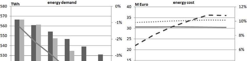
9. Internationale Energiewirtschaftstagung an der TU Wien                                                                                                                                IEWT 2015

Die Arbeitsplatzeffekte werden mit Hilfe der Sattelitenaccounts des statistischen
Bundesamtes berechnet. In den Sattelitenaccounts sind den Löhnen und Gehältern aus der
IO-Tabelle die Anzahl der Arbeitnehmer (Vollzeitäquivalente) und die Anzahl der
Erwerbstätigen1, unterschieden nach Sektoren, zugeordnet. Dadurch ergibt sich für die
Arbeitsplatzeffekte eine andere Entwicklung als für die Wertschöpfungseffekte.
Ergebnisse und Schlussfolgerungen
Die Gebäudemodellierung ergab einen zusätzlichen Investitionsbedarf von 6,88 Mrd.
EUR2010. Bei einem Anteil von 26,4% Vermietern ergibt sich dadurch einen Mehrkonsum
des Bankensektors von 241 Mio. EUR2010 sowie 2,20 Mrd. EUR2010 an Mehrausgaben für
Miete.
Die größten positiven Effekte auf die Wertschöpfung gab es erwartungsgemäß im Bausektor
mit einer Steigerung von 7,9% (bezogen auf die Tabelle von 2007, siehe Abbildung 1). Auf
Rang zwei und drei der größten Effekten stehen mit sinkender Wertschöpfung die
Energiesektoren Strom- und Fernwärme (-8,7%) sowie Kohle (-7,3%), was auf die
Energieeinsparungen zurückzuführen ist. Das zweitgrößte Wachstum zeigt der Sektor
Wohnungswesen mit 1,1%. Ursache hierfür ist die Kapitalfinanzierung der
Effizienzmaßnahmen durch Miete. Die Sektoren Holz- und Kunststoffwaren und Anlagen
(Geräte) für die Stromerzeugung sind Vorleistungen für den Bausektor, wobei letzterer mit
z.B. Kabeln, Schaltern und Leuchten den größten Anteil der Vorleistungen beiträgt. Die
Effekte in diesen Sektoren sind daher indirekt und fallen deutlich schwächer aus. Bei den
Erwerbstätigen dominiert der Wachstumseffekt im Bausektor noch deutlicher aufgrund des
hohen manuellen Arbeitseinsatzes im sektoralen Vergleich.
                                  10                                                                                              120
                                                                                     Erwerbstätigenänderungen in Tsd. Personen*

                                   8
                                                                                                                                  100
Wertschöpfungsveränderung* in %

                                   6

                                   4                                                                                               80

                                   2
                                                                                                                                   60
                                   0
                                                                                                                                   40
                                   ‐2

                                   ‐4                                                                                              20

                                   ‐6
                                                                                                                                    0
                                   ‐8
                                        * unter Verwendung der IO‐Tabelle von 2007                                                                              * unter Verwendung der IO‐Tabelle von 2007
                                  ‐10                                                                                             ‐20

Abbildung 1: Ergebnisse der                                                 sektoralen                                                  Wertschöpfungs-   und       Arbeitsplatzeffekte                      der
Gebäudeeffizienzmaßnahmen

Im Jahresvergleich zwischen den Basisjahren 1995 bis 2007 unterscheiden sich die
Wertschöpfungs- und Arbeitsplatzeffekte kaum in ihrer Richtung, aber in ihren quantitativen
Effekten, wie Abbildung 2 zeigt. Die Impulse der betroffenen Sektoren fallen umso stärker

1
  ebenfalls Vollzeitäquivalente aber beinhaltet neben den Angestellten auch die
Selbständigen

                                                                                     Seite 2 von 20
9. Internationale Energiewirtschaftstagung an der TU Wien IEWT 2015
aus, je weiter die Input-Output-Tabellen zurückliegen, weil die betroffenen Sektoren in den
älteren IO-Tabellen einen größeren Anteil an der Gesamtwertschöpfung einnehmen.
Interessant für weitere Analysen wäre eine Unterscheidung nach Preiseffekten und
technischem Fortschritt, was zusätzlich zur klassischen Input-Output-Analyse ergänzende
Mengengerüste und sektorale Preisniveaus erfordert.
0.40
0.35
0.30
Veränderungen im Vergleich zur Basis in %
0.25
0.20
0.15
Produktionswert
0.10 Erwerbstätige
Arbeitnehmer
0.05 Nachfrageimpuls
0.00
1995 1996 1997 1998 1999 2000 2001 2002 2003 2004 2005 2006 2007
Input‐Output‐Tabelle des Jahres ...
Abbildung 2: Vergleich der Gesamteinflusses der verschiedenen Input-Output-Jahrestabellen
Literatur
[1] Diefenbach, Nikolaus; Cischinsky, Holger; Rodenfels, Markus; Clausnitzer, Klaus-Dieter (2010): Datenbasis
Gebäudebestand. Datenerhebung zur energetischen Qualität und zu den Modernisierungstrends im deutschen
Wohngebäudebestand. 1. Aufl. Institut Wohnen und Umwelt GmbH (IWU). Darmstadt
[2] Öko Institut, Fraunhofer ISI: Klimaschutzszenario 2050. Erste Modellierungsrunde. Studie im Auftrag des
Bundesministeriums für Umwelt, Naturschutz, Bau und Reaktorsicherheit. Berlin, 2014.
[3] Miller, Ronald E.; Blair, Peter D (2009): Input-output analysis (2. ed.). Foundations and extensions. Cambridge Univ. Pr.
Keywords: Building insulation, Input-Output analysis, sensitivity analysis
1 Introduction
Assessing sectoral macroeconomic policy effects is generally based at least partially on
some sort of Input-Output (IO) model (West, 1995). IO tables are published on a yearly basis
in all Western countries offer a statistical description of production interdependencies and
demand quantities of an economy (Miller and Blair, 2009). The industry linkages are found in
the technical coefficients, showing the value of sectoral intermediate inputs to gross outputs
of each sector. IO tables are published in matrix forms.
Seite 3 von 209. Internationale Energiewirtschaftstagung an der TU Wien IEWT 2015
However, since IO models are a mere statistical description of an economy, the technical
coefficients of a given year, supposed to represent the production recipes of one sector, are
prone to changes. Analyses over longer horizons which are based on one single year can
give a less accurate picture of the impacts of policy chances. IO analysis in its basic form is
static and transforming them into truly dynamical models requires a change in the technical
coefficients (Leontief and Duchin, 1986). Those coefficients can change quite substantially,
even for some industries, which are rather stable in their production technology, like the
construction sector (Pietroforte and Gregori, 2003). While there are possibilities to alter these
coefficients, Richter (1991) has shown in his overview that reasons for a change in those
technical coefficients may be due to technical changes in general, price changes or changes
in the product mix.
An understanding of how these coefficients may change over time requires a deep
understanding of the production technologies currently present in the sector as well as
forecasts or assumptions on future developments of those production technologies. If one is
concerned about the development of more than one sector at once, these technological
changes can become overwhelmingly difficult. Usually, this is the case in impact assessment
studies. Not only do effects compound, they overlap, and it requires more than detailed
insights into the structural composition of the sectors in question. This is more than often
asked for too much.
In this paper we embarked on this problem by another approach: we modelled future energy
demand in Germany’s residential buildings in a base2 scenario (Repenning et al., 2014), then
tried to achieve the heat demand reduction goal for 20203 as stated in the national energy
concept in an alternative scenario (BMU, 2011). The difference between those two scenarios
represents the impulse on the macro economy and is finally fed into a series of IO-tables
(Destatis, 2010) for a conventional static IO-analysis (Miller and Blair, 2009). The IO-tables
from the Federal Statistical Office served as a kind of sensitivity analysis of the
macroeconomic changes imposed by the detailed sectoral model of the real estate sector.
The changes in the detailed model of the housing sector, which we call for convenience
bottom-up model (bum) in the remainder,4 do not only concern the construction sector as
deliverer of building insulation installation services (the material required for this is supposed
to be contained in the intermediate deliveries of the construction sector). The bum changes
impact also on energy demand (which ought to be negative, as stated by the reduction
goals), rents and financial services for financing the extra insulation.
2
In the base scenario policy measures implemented until September 31st 2012 were
considered.
3
The heat reduction of 20% until 2020 was not to be achieved with realistic retrofit rates,
thus we arranged the scenario to stay on track for the 2050 primary energy reduction goal of
80%
4
We defined the notion of bottom-up due to the concrete demand forecasts, which in the
model of the housing sector is microeconomic, while Input-Output tables are
macroeconomic.
Seite 4 von 209. Internationale Energiewirtschaftstagung an der TU Wien IEWT 2015
2 Methods
The heat demand was simulated with the model EE-Lab/INVERT, using the German building
stock of 2010 with updates for retrofit action from Diefenbach et al. (2010). A detailed
description of the model can be found in Kranzl et al. (2013)5.
The scenario was constructed according to the climate protection scenario 2050, a study for
the German Federal Ministry for the Environment, Nature Conservation, Building and Nuclear
Safety (Repenning et al., 2014). This report provides a detailed description of the
assumptions underlying this scenario regarding socio-economic developments like economic
growth, energy prices and population development. The energy saving goals of the German
government for 2020 defined the investment requirements for insulation in that scenario.
2.1 From efficiency measures to macroeconomic impulses
We restricted our analyis on only residential living space is included in the analysis, as
shown in the owner-user scheme of the building stock given in table 2-1. Non-residential
buildings and spaces are excluded, for several reasons. First, the buildings vary considerably
in their use and energy demand. In addition, more assumptions are necessary to cover the
investment decision processes of companies. Finally, company tenant payments are
intermediate inputs in the Input-Output (IO) tables and a true consideration would require a
manipulation of the technical coefficients. Though a manipulation of the matrix of
intermediate deliveries can be done with RAS-like algorithms (Junius and Oosterhaven,
2003), this is contra productive for a main focus of this paper: assessing the effect of using
IO tables from different years with the same policy impulses.
We have identified, that the energy saving measures chosen by the investor, which is mostly
the owner, have the following impulses on the macro economy.
investments cause the final demand (investment for firm-owned facilities and
consumption for private households)6 in the building sector to go up
financing the investment causes additional final demand (consumption) in the credit
businesses
increase of the rent accumulated over time causes an increase final demand in real
estate / housing (consumption)
5
www.invert.at
6
Note here that there is distinction between the microeconomic understanding of
investments, which are financial commitments whose use extends over a longer period and
the macroeconomic understanding of investments, which is done by firms. All financial
payments done by private households are categorized as consumption in macroeconomics.
Seite 5 von 209. Internationale Energiewirtschaftstagung an der TU Wien IEWT 2015
energy savings reduce the final demand (consumption) in the energy sector
2-1: owner-user scheme for buildings
owner
private housing other
household industry companies
poo
private
owner-
household n/a n/a
occupier
private owner-
household occupier
user p2p h2p not in scope:
tenant private-to- housing-to- industry
private private buildings
owner-
not in scope:
companies occupier n/a
non-residential use
tenant
The private household as an owner-occupier invests in a measure increasing the energy
efficiency of the building envelope or in a renewable heating system. In the year of the
implementation of the measure the whole investment flows into the building installation
sector (CPA 45.3 - 45.5). Thus, final demand for building installations in the consumption of
the private households grows. In the following years, the private household saves energy
cost due to the implemented measure. Therefore, the expenditures for energy (CPA 40, 10)
rise in the consumption vector. For financing the investment there are three sources.
Energetic retrofit is supported by the government through subsidies. Another part of the
investment can be financed by credits and the rest from private savings. We assume that
50% of the investment is financed through credits. The service fee charged by the credit
intermediary is assumed to be 7% of the credit volume. This charge represents the impact on
the credit business’ final demand (CPA 65) in the year of the investment. The second
financing source, the savings, reduces the private households’ capital and may also lead to a
calculated value increase of the building. However, both of these effects are genuinely only
included in flow-of-fund analysis of national accounts, which are not published as regularly as
IO tables.7 Apart from that, the main impact of public subsidies - the third financing source -
takes place in the decision making phase for energetic retrofit, happening prior to the
7
A Social Accounting Matrix (SAM) for Germany was officially only published for the year
2000. It would have been inconsistent using Io tables differing yearly and one single SAM.
Seite 6 von 209. Internationale Energiewirtschaftstagung an der TU Wien IEWT 2015
macroeconomic impact. Thus, the effect of subsidies on the macro economy is not in the
scope of this analysis.8
When a private landlord invests in efficiency measures in buildings the same approach is
taken with one addition: the increase in rent for energetic improvement. In the years following
the landlord, thus, receives up to 11% of the expenses according to BGB §559. These
additional rental expenses of the private occupier increase the consumption of the private
households for services for real estate and housing (CPA 70). We assumed that the landlord
elevates the rent by the maximum allowed, i.e. 11%. In reality, such an increase can not
always be realized, for example in shrinking areas. However, we need to use this rate, since
empirical data is not available.
2-2 CPA-No. and sector description
CPA-No. Sector description
10 Mining of coal and lignite
20 Manufacture of wood and wood products
25.2 Manufacture of plastic products
28 Metal products
31 Manufacture of electrical machinery and apparatus
40.1, 40.3 Electricity and steam supply
40.2 Gas manufacture and distribution
45.3 – 45.5 Building installation
51 Wholesale trade
52 Retail trade
60.1 Railway transport
65 Financial intermediation
67 Activities auxiliary to financial intermediation
70 Real estate activities
74 Other business activities
75.1 – 75.2 Public administration and defense
8
It could be argued that subsidies would alter the primary input matrix of the IO tables, but
this would not affect the construction sector, only the sector of rental services. Since we
deduct those subsidies from the increase of rents we made sure that the subsidies did not
artificially increase our results.
Seite 7 von 209. Internationale Energiewirtschaftstagung an der TU Wien IEWT 2015
How does the investment influence the macroeconomic impulse if the landlord is a housing
association or company instead of a private owner? In contrast to the investment of a
private landlord, the investment of a company does not affect the consumption vector but
increases the capital investment in the building sector.
The final demand impulse, shown for 2010 in table 3, is the interface between the bottom-up
building simulation and the macroeconomic calculation.
2-3 Final demand impulse for 2010
Sector Additional expenses (in Mio. EUR2010)
Building installation 8,670
Electricity and steam supply -5,690
Financial intermediation 303
Auxiliaries to financial intermediation 3,665
2.2 From impulse to macroeconomic impact
For evaluating the macroeconomic impact we used the static Input-Output model (IO-model),
according to Holub and Schnabl (1994). The model
xt = Atxt + yt (1)
with At as the matrix of intermediate inputs and yt as the final demand vector of a given year
t. This model has the solution
x = (I - A)-1y (2)
(or x = Ly with the matrix M ≡ (I - A)-1 as the Leontief inverse) (Miller and Blair, 2009).
The current final demand vector yt consists of invest, consumption, government expenditures
and exports.
y = I + C + G + Ex (3)
It results from statistical data supplied by the German Federal Statistical Office (Destatis,
2010). We change the consumption component of this final demand vector using the
investment data for energy efficiency measures in buildings from the simulation model,
according to the final demand impulse scheme, as given by table 3. This new final demand
vector ytN results from the deduction of savings in heating expenses (h) and the addition of
the extra expenses for insulation (i), credit services (c) and rents (r). The subscript t denotes
the (base) year of the Input-Output-table, ranging from 1995 to 2007.9 The expenditure
changes are deflated to every year t with a common deflator d for all e:
9
A detailed explanation for the choice of this period is given below.
Seite 8 von 209. Internationale Energiewirtschaftstagung an der TU Wien IEWT 2015
ytN = yt + dt[ei,c,r - eh] (4)
The change to the elements of the final demand vector ytN is described in detail in section
2.1, where each of the items from the list 2.1 corresponds to a value in e.
While ytN is given with price levels of the (base) year t, the inputs ei,c,r,h are given in price
levels of 2010, as the model of the real estate sector is calibrated against this year. Thus, we
inflated ei,c,r,h to each of the years t of the Input-Output-tables with a deflator dt. Since we are
mainly interested in changes evoked by the model (the additional extra expenses are the
direct effects and the model gives the indirect effects of the policy changes), we calculated
the respective ∆v for gross value added (GVA), which is given by the following equation:
∆v = v’ (I - A)-1 ytN /v’ (5)
After having obtained ∆v, these values were inflated with 1/dt to the price level of 2010 for
making the results comparable. We used the overall price level of the German Federal
Statistical Office, sine no official data on sectoral price levels in the required classification are
published. Furthermore, while an aggregated price level would seem desirable, it imposes
some serious problems in the price corrections of the inter-industry relationships, something
which we avoided by our approach. Nevertheless, there remains a problem of how to
distinguish changes in the quantity, prices and inflation, whose variations are normally
eliminated congruently, using the Laspeyres price chain index (Reich, 2008).
Sectoral labour requirements are published as a satellite account by the Federal Statistical
Office (in the primary input matrix only aggregate wages payments are found), which is the
row vector l’ (both for employed persons and employees). Underlying these figures is
sectoral labour productivity. Calculating the direct and indirect additional labour requirements
by the policy changes is done by the following equation (Leontief, 2008):
∆l = l’ (I - A)-1 ytN /l’ (6)
For the sensitivity analysis we vary the macroeconomic data set A by base year t. The varied
data sets form different starting points for the IO-Analysis. Our intent is to measure how
much the resulting sectoral gross output and employment will vary.
Thus, we applied the same (inflated) input data on the IO-tables from the Federal Statistical
Office from 1995 to 2007. Within this time span, the same sector classification (WZ 2003)
was used (Destatis, 2008). We decided not to extend the analysis to the IO-tables from 2008
to 2010, since it would have been necessary to split two of our input data:
the sector for generating electricity and heat, CPA (Classification of Products by
Activity) Code 40.1-40.3 (WZ 2003) is in the new classification (WZ2008) split into
CPA Code 35.1, 35.3 (grouped) and 37-39 and
the sector for renting CPA 70 (WZ 2003) is split into CPA 41 (WZ 2008) and CPA 68
(WZ 2008).
While especially for the latter case it could be argued that the effects of splitting are minor, as
the share which ought to be put into CPA 41 (WZ 2008), we do not want to produce any
artifact of the indirect effects of the impulses. Furthermore, it would be hard to distinguish
between the effects resulting from an updated data base and the effects which come from a
different sectoral classification.
Seite 9 von 209. Internationale Energiewirtschaftstagung an der TU Wien IEWT 2015
Figure 1: Impulse flow in the IO-Table
For the illustration of the macroeconomic impact we chose the change in gross value added
and the gross output. The gross value added, is the value the sector directly produced
excluding the value that other sector generated previously. Whereas, the gross output shows
what each sector produces including the intermediate inputs. In other words: gross value is
gross output minus intermediate inputs.
The direct impacts of the additional investment are for example the building sector receiving
the retrofit investment or the energy sector loosing energy demand and income. These
effects are included in the final demand vector shown in table 3. Indirect effects are
calculated by employing equations 5 and 6 on the complete IO-Table. An increase in the
building sector will affect the dependent sectors, like manufacture of wood and wood
products sector and as their input requirements grow other sectors might be affected. These
indirect effects are included in the gross value added and in the gross output.
3 Results of the bottom-up building simulation
To analyze the effect of additional measures in energy efficiency in buildings, we need to
compare the KS80, reflecting the German energy saving goals, to a base scenario (base)
Seite 10 von 209. Internationale Energiewirtschaftstagung an der TU Wien IEWT 2015
including only political action that has been decided on as of 31.September 2012. Figure 2
shows the steeper decline in KS80 as it spreads away from the base scenario ending up with
a difference of -5.5%. Interpreting these data, we have to keep in mind that the additional
efficiency measures in this scenario only kicked off in 2014. Thus, the 5.5% additional
savings represent 6 years of efficiency measures, where each year another approximately
1% of the stock. Each of these years more, additional annual energy savings are
accumulated, in this case almost 1%. This is will continue for 20 - 30 years based on the
retrofit and heating system exchange rate, since the measures have such long lasting effect.
Caused by the decrease in energy demand but also by the fuel switch, the energy savings
rise up to 11% until 2020, see figure 2. In absolute numbers the energy cost shift, meaning
that rising energy prices balance out the shrinking energy demand.
Figure 2: Energy demand (left) and energy cost (right) for KS80 and base scenario and percentage
difference
In all sectors the consumption of the private households outweighs the investment of
companies due to the higher share of privately owned buildings, i.e. around 80% of the living
space. The additional energy efficiency measures in scenario KS80 lead to an increased
annual national expenditure of 8.8 billion Euros in 2015 and similarly 8.7 billion Euro in 2020.
This includes the both expenditure categories, those of private households affecting their
consumption and those of companies increasing their investment. The term investment in the
national accounting meaning of the word only includes those expenditures that are made by
companies, where "investments" by private households are included in the consumption
section. This differentiation is made for further macroeconomic analysis, that may use the
data for an in depth review. In the building installation the consumption the households is
lower in 2015 that in 2020, whereas, the investment of the companies increase.
This is not a systematic development, but rather a temporary glance reflecting the additional
building expenses of one scenario compared to another. In the AMS scenario the renovation
rate was carried forward in a "natural" development dependent on the building age. In the
Seite 11 von 209. Internationale Energiewirtschaftstagung an der TU Wien IEWT 2015
KS80 scenario the renovation rate was increased starting in 2014 trying (and failing) to
achieve the 2020 savings goal. Thus, the retrofits were many and the investments already
quite high in 2015. Hence, from 2015 to 2020 the number of retrofits did not increase as
much in the KS80 compared to the AMS. Subsequently the additional investment is also
lower.
The financial intermediation with its credit business development follows the one of the
building installation sector, due to the tie through constant parameters, the share of financing
and the profit margin, for both households and companies. The total real estate activities,
that is the sector including the rents, grow at the about same 170% as the energy savings
between 2015 and 2020.
3-1 Consumption and investment impulses
Sector Additional effect 2015 MEuro 2020 MEuro
Building installation consumption 8,107 6,884
investment 712 1,786
total 8,819 8,670
Financial intermediation consumption 284 241
investment 25 62
total 309 303
Real estate activities consumption 1,283 2,198
investment 922 1,467
total 2,205 3,665
Electricity and steam supply consumption -3,388 -5,690
4 Results of the macroeconomic analysis
Gross output, represented by the solid line in figure 3, increases by 0.34% in 2020 when
applying the IO-Table of 1995, i.e. assuming that the national economy in 2020 will be
structured like in 1995. The illustration shows the declining impact of the efficiency measures
when the different structures of 1995 until 2007 are assumed. Applying the IO-Table of 2007
merely leads to an increase of 0.206%. The impacts on employed persons and employees10
are both declining, though the gap between the two widens, being 0.01 percentage points
with the table of 1995 and 0.53% with the one of 2007. It seems like the indirect effects
cause more freelancers to be employed.
10
Employed persons include freelancers
Seite 12 von 209. Internationale Energiewirtschaftstagung an der TU Wien IEWT 2015
Figure 3: Changes compared to each baseline year
Final demand development represents the direct effect or the impulse (or ytN in equation 4).
So there is a shrinking impact of the direct effects over time, which is only a result of a
different composition of y in equation 3. Indirect effects are calculated with equations 5 and 6
for gross value added and employment and include both the direct effects and changes due
to the different intermediate delivery matrices in the base years (the A-matrix of equation 1).
While indirect impacts are higher, using the IO-Tables from 1995 to 2001, the picture
changes after 2001: the impact on gross output is lower than the final demand impulse. This
is due to the growing influence of the energy savings, causing a higher effect on gross output
over time. In addition, the input coefficients of the IO-tables provide further explanation. The
construction sector needs less intermediate deliveries in 2007, i.e. 42.6% of the gross output
of the sector, than in 1995, 54.3%. In the energy sector a reverse trend can be observed with
the share in 1995 being 41.2% of its gross output and 49.2% in 2007, indicating that the
indirect effects triggered by this sector rise.
Not only the share of intermediate inputs changes; the structure of the coefficients changes
as well. Analyzing the energy sector, the total input share of the coal sector is 14.7% in 1995
compared to 4.7% in 2007. There is a shift of energy carriers away from coal towards gas
and electricity. The intra-industry production within the energy sector, i.e. the intermediate
deliveries that remain within the sector, has a share of 1.6% in 1995 compared to 19.3% in
2007. This development of indicators indicates that over time the own energy need of the
sector increases.
The declining impact is not resulting of a decline in importance of the sectors which received
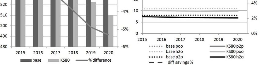
an impulse, as can be seen from figure 4. The share of the sectors of overall private
consumption is relatively stable; for real estate activities it is around 20%, for financial
intermediation between 3% and 4%, for building installation between 4% and 5% and, for the
sector receiving a negative impulse, electricity and steam supply, it is around 2%.
Seite 13 von 209. Internationale Energiewirtschaftstagung an der TU Wien IEWT 2015
Figure 4: Sectoral consumption shares
This means, on the other hand, that the declining overall impact of the suggested policy
impulses is mostly due to changes in the matrix of intermediate deliveries (the A-matrix in
equation 1). Apparently, the sectors involved in the final demand change trigger less and less
intermediate deliveries. Nevertheless, the basic structure of production does not change
fundamentally, as a common fundamental structure of production in modern economic
systems is supposed (Simpson and Tsukui, 1965). This becomes evident in the following
detailed analysis of sectoral changes in gross value added and employment.
Figure 5: Changes in sectoral gross value added
Seite 14 von 209. Internationale Energiewirtschaftstagung an der TU Wien IEWT 2015
Figure 5 gives the resulting changes of sectoral gross value added for the Input-Output-table
of 2007, which has been calculated with equation 5. The solid stacks are the values obtained
by using the Input-Output-Table from 2007; the thin lines give the range (minimum and
maximum values) and averages for all analyses from 1995 and 2007. We only showed
sectors with a change either bigger or lesser than 0.5%. The numbers are the CPA-numbers
of the sectors.
What can immediately be seen from figure 5 is that the values for the table from 2007 are in
the majority of cases the minimum from all analyses. This observation is quite in line the
aforementioned decreasing impact of the policy changes, due to a lesser weight of the
sectors included in the direct impacts.
Figure 6: Changes in sectoral requirements for employed persons
The direct and indirect impacts on employed person requirements on a sectoral level are
given by figure 6. They have been calculated by equation 6. We only considered sectors with
a change bigger than 1500 or less than minus 500 persons.
5 Discussion
The results of the Input-Output analysis indicate that the construction sector is above-
average interrelated in the economy, if one looks at the average of intermediate delivery
input share of all sectors, compared to overall production. Where the average over all sectors
from 1995 and 2007 is between 0.419 and 0.447, the input share for the building installation
sector is between 0.526 and 0.573. Thus, the building installation sector is among the 20% of
the most interrelated sectors in the German economy.
Seite 15 von 209. Internationale Energiewirtschaftstagung an der TU Wien IEWT 2015
This is supported by the findings from Pietroforte and Gregori (2003), who showed for the
German pre-reunification period a larger impact for the German construction sector,
compared to other OECD countries. The peak in 2005 of overall production output can be
interpreted as a statistical artifact of the building boom, something which is even more
striking regarding the subsequent relative decline of the production output gain.
The analysis for a single year is blurred by cyclical behaviour of the economy. Recognizing
such business cycles is a general problem in macroeconomic analysis. A business cycle can
be characterized by an expansion and a subsequent contraction, the former separating the
latter by a peak and a trough, reversely, and lasts on average about 7 years, with 6 years of
expansion and 1 year of recession (Mostaghimi, 2010). While taking account of the period
from 1995 to 2007 in our analysis, these 13 years would be roughly equivalent to 2 full
business cycles. So while analyzing different IO-tables, it may be possible leveraging out the
influence of the business cycles on our results with average values. This supports a higher
robustness of the results. Furthermore, the real estate market (and its immense impact on
the construction sector) is probably prone to a time lag from the overall business cycle
(Schmoll, 2007).
Usually, the demand for housing services is income-dependent and changes both in income
and prices are depicted by the income elasticity of demand (Schmoll, 2007). The same
usually applies to other demand categories, but with different income elasticities. In our
analysis we did not account for possible elasticity changes, so demand is totally inelastic in
our case. This is not uncommon for IO analysis, since they do not refer to any underlying
microeconomic model. However, in going from a static IO-based model to a dynamic model,
this feedback effect should be accounted for (and also possible rebound effects from energy
savings (Berkhout et al., 2000)). It should be noted, though, that this would require the real
estate market being a perfect market, which is quite far from reality (Schmoll, 2007).
Energy demand reduction was calculated as a percentage change from the electricity and
steam supply sector (see equation 4). A simplification was chosen as those sectors also
contain electricity and steam distribution, whose demand admittedly does not shrink linearly
with overall electricity demand. However, since no better data basis was available to account
for this fact, this simplifying approach was justified. Furthermore, the standard assumption in
IO-analysis is operation under full capacity utilization, so it is hard to find a better way with
dealing with this fact in the theoretical framework of the static IO-analysis. Distributional
demand from non-consumers is part of the intermediate delivery matrix of the respective
sector, supporting our linear approach.
Ecological modernisation measures are treated no other than general real estate
modernisation and annually 11% of it can be assigned to rent increases, according to §559
BGB. However, interest subsidy loans have to be accounted for (Jaeger, 2014). Since this
decision is subject to the current price level in the region of the real estate and the socio-
economic situation of the tenant has to be accounted for, it is not always given that rents
increase accordingly. Thus, there is some uncertainty in this decision, which we cannot
consider in our analysis.
The matrix of technical coefficients, which is the first (and main) driver for inter-temporal
differences in gross value added changes, is, like the whole Input-Output-model, descriptive
and not normative. That is, an efficient allocation of goods is already assumed, as well as full
Seite 16 von 209. Internationale Energiewirtschaftstagung an der TU Wien IEWT 2015
capacity utilization. This is important to notice, since changes in the technical coefficients
may stem wither from volume changes (which is equivalent to a change in the production
recipes of the sectors) or from price changes of the intermediate goods (Richter, 1991).
However, with only taking the official Input-Output-tables as analytical device, it is not
possible to separate these two effects.
The size of the manipulated sectors being the second driver for intertemporal differences in
gross value added changes leaves room for interpreting the consumption shifts in observed
utility. However, this needs a much more thorough inspection and interpretation as what this
analysis could possibly deliver. An analysis is not possible to do with solely relying on
aggregate data, such as a representative household. Different household types are known to
exhibit quite different consumption patterns (Wier et al., 2001), which are heavily influenced
by income, but also by other socio-cultural and demographic factors as e.g. household size.11
Furthermore, possible price effects in the final demand vectors can also only be separated if
one possesses additional information.
6 Conclusions
Based on the results presented in sections 3 and 4 we quantified the gross economic output
and the number of employed persons to grow about 0.27 % and 0.30 % on average, caused
by additional energy efficiency measures in buildings. We also found that the effect
decreases over time due to the structure of the economy as represented by the different
Input-Output (IO)-Tables. Thus, the impact on the gross output shrinks by 0.13 %pts,
whereas the number of employed persons only shrinks from 0.35 % to 0.28 %, depending on
base year macroeconomic structure. This overall impact on the macro economy mainly
triggered by an 8.3 % increase of the gross value added in the buildings sector, whilst the
energy sector decreases by around 8%.
We consider two implications of the presented results. Firstly, the positive macroeconomic
impact can contribute to the profitability of building retrofit. Due to their large investment and
long cycle efficiency measures in buildings are often unattractive with inherent long term risk
and, if ambitious, possible failure to be profitable for the investor. However, the invested
money is not lost; it is fed back into the economy and leads to increased production and
employment. Secondly, when comparing different studies assessing the macroeconomic
impact of measures in the building sector, one has to be aware of the range of 0.07%pts
(employed persons) to 0.13%pts (gross output) that results vary depending on the year they
are based on. This error range is only valid for the building in Germany and base years
between 1995 and 2007. We did not cover product or process improvements that are
triggered by increased production, i.e. retrofit.
11
The impact of socio-cultural variables on energy consumption is of minor importance (Wier
et al., 2001), but placement does play a role.
Seite 17 von 209. Internationale Energiewirtschaftstagung an der TU Wien IEWT 2015
Our method has its clear limitations: static IO-analysis cannot take price effects into account
which constitute a feedback from price changes (and possible economies of scales) to
physical quantities, which is excluded by the Non-Substitution Theorem imposed by the
production function (Duchin and Steenge, 2007). This limitation is also important concerning
income elasticity effects for the consumer, which would have to be implemented
exogenously. Finally, aggregation errors are also unavoidable in IO-studies (Rueda-
Cantuche et al., 2013) and one could consider splitting the energy savings to different
sectors. We decided not to as this would have imposed further assumptions on the interface
between the bottom-up model and the IO-table.
Capital flows are not part of the official IO-publications from the German Federal Statistical
Office, so we had to establish own assumptions on capital flow effects. Furthermore, we did
not extend our analysis to the most recent IO-tables, since they are published with a different
classification of economic sectors. We could not distinguish in our analysis whether observed
effects are caused by price or quantity changes, which is only possible with a decomposition
analysis drawing on further external assumptions. We restricted our analysis to changes in
2020. The bottom-up model would allow further time steps, but since IO-analysis becomes
less accurate over time, the evaluation of effects becomes less valid.
The limitations of our study are also beneficial as the results are easily reproducible and we
are not concerned with the validity of external assumptions since we stick strictly to the basic
framework. Nevertheless, our approach of using a time series of IO-tables offers one
cornerstone for a challenge to the vast majority of IO-studies: the issue of sensitivity analysis
(Dietzenbacher et al., 2013). Normally, IO-studies (or studies based on the IO-methodology,
like CGE models (Rose, 1995)) either take the last table published or a table in a year where
business cycle influences are thought to be minimal. We conclude that our approach gives
more insight and a more balanced view of possible indirect macroeconomic effects.
References
Berkhout, H., Muskens, J. C., and Velthuijsen, J. W. (2000). Defining the rebound effect.
Energy Policy, 28:425–432.
BMU (2011). Das Energiekonzept der Bundesregierung 2010 und die Energiewende 2011.
Technical report, Bundesministerium für Umwelt, Naturschutz und Reaktorsicherheit -
Federal Ministry for the Environment, Nature Protection and Nuclear Safety.
Destatis (2008). Klassifikation der Wirtschaftszweige mit Erläuterungen. Technical report,
Statistisches Bundesamt (Federal Statistical Office).
Destatis (2010). Volkswirtschaftliche Gesamtrechnungen. Input-Output-
Rechnung. Fachserie 18 Reihe 2, Statistisches Bundesamt (Federal Statistical Office).
Diefenbach, N., Cischinsky, H., Rodenfels, M., and Clausnitzer, K.-D. (2010). Datenbasis
Gebäudebestand. Datenerhebung zur energetischen Qualität und zu den
Modernisierungstrends im deutschen Wohngebäudebestand. Technical report, Institut
Wohnen und Umwelt GmbH (IWU).
Seite 18 von 209. Internationale Energiewirtschaftstagung an der TU Wien IEWT 2015
Dietzenbacher, E., Lenzen, M., Los, B., Guan, D., Lahr, M. L., Sancho, F., Suh, S., and
Yang, C. (2013). Input-output analysis: the next 25 years. Economic Systems
Research, 25(4):369–389.
Duchin, F. and Steenge, A. E. (2007). Mathematical models in input-output economics.
Rensselaer Working Papers in Economics, 703:1–32.
Holub, H.-W. and Schnabl, H. (1994). Input-Output-Rechnung: Input-Output-Analyse.
Einführung. Oldenbourg.
Jaeger, G. M. (2014). Wohnraummiete. In Usinger, W. and Minuth, K., editors, Immobilien,
Recht und Steuern. Handbuch für die Immobilienwirtschaft, volume 4. Boorberg.
Junius, T. and Oosterhaven, J. (2003). The solution of updating or regionalizing a matrix with
both positive and negative entries. Economic Systems Research, 15(1):87–96.
Kranzl, L., Hummel, M., Müller, A., and Steinbach, J. (2013). Renewable heating:
Perspectives and the impact of policy instruments. Energy Policy, 59:44–58.
Leontief, W. (2008). Input-output analysis. In Durlauf, S. N. and Blume, L. E., editors, The
New Palgrave Dictionary of Economics, volume 4. Palgrave Macmillan.
Leontief, W. and Duchin, F. (1986). The future impact of automation on workers. Oxford
University Press.
Miller, R. E. and Blair, P. D. (2009). Input-Output analysis. Foundations and extensions.
Cambridge University Press, 2 edition.
Mostaghimi, M. (2010). Economic measurement and forecasting. In Free, R. C., editor, 21st
century economics: a reference handbook, number 1, pages 287–295. Sage
Publications.
Pietroforte, R. and Gregori, T. (2003). An input-output analysis of the construction sector in
highly developed economies. Construction Management and Economics, 21:319–
327.
Reich, U.-P. (2008). Additivity of deflated input-output tables in national accounts. Economic
Systems Research, 20(4):415–428.
Repenning, J., Matthes, F., Blanck, R., Emele, L., Döring, U., Förster, H., Haller, M., Harthan,
R., Henneberg, K., Hermann, H., Jörß, W., Kasten, P., Ludig, S., Loreck, C.,
Scheffler, M., Schumacher, K., Eichhammer, W., Braungardt, S., Elsland, R., Fleiter,
T., Hartwig, J., Kockat, J., Pfluger, B., Schade, W., Schlomann, B., Sensfuß, F.,
Athmann, U., and Ziesing, H.-J. (2014). Klimaschutzszenario 2050. 1.
Modellierungsrunde. Studie im Auftrag des BMUB. Technical report, Öko-Institut,
Fraunhofer ISI.
Richter, J. (1991). Aktualisierung und Prognose technischer Koeffizienten in
gesamtwirtschaftlichen Input-Output-Modellen. Physica-Verlag.
Rose, A. (1995). Input-output economics and computable general equilibrium models.
Structural Change and Economic Dynamics, 6:295–304.
Seite 19 von 209. Internationale Energiewirtschaftstagung an der TU Wien IEWT 2015
Rueda-Cantuche, J. M., Dietzenbacher, E., Fernández, E., and Amores, A. F. (2013). The
bias of the multiplier matrix when supply and use tables are stochastic. Economic
Systems Research, 25(4):435–448.
Schmoll, F. (2007). Staat und Markt - die volkswirtschaftliche Perspektive. In Fritz Schmoll, c.
E., editor, Basiswissen Immobilienwirtschaft, volume 2. Grundeigentum-Verlag.
Simpson, D. and Tsukui, J. (1965). The fundamental structure of input-output tables, an
international comparison. The Review of Economics and Statistics, 47(4):434–446.
West, G. R. (1995). Comparison of input-output, input-output + econometric and computable
general equilibrium impact models at the regional level. Economic Systems
Research, 7(2):209–227.
Wier, M., Lenzen, M., Munksgaard, J., and Smed, S. (2001). Effects of household
consumption patterns on CO2 requirements. Economic Systems Research,
13(3):259–274.
Seite 20 von 20You can also read