Machine Learning Regression Model for Predicting Honey Harvests - MDPI
←
→
Page content transcription
If your browser does not render page correctly, please read the page content below
agriculture
Article
Machine Learning Regression Model for Predicting
Honey Harvests
Tristan Campbell 1, *, Kingsley W. Dixon 2 , Kenneth Dods 3 , Peter Fearns 2 and
Rebecca Handcock 4
 1    Computing and Mathematical Sciences, School of Electrical Engineering, Curtin University,
      Perth 6102, Australia
 2    School of Molecular and Life Sciences, Curtin University, Perth 6102, Australia;
      kingsley.dixon@curtin.edu.au (K.W.D.); peter.fearns@curtin.edu.au (P.F.)
 3    Chem Centre, Perth 6102, Australia; KDods@chemcentre.wa.gov.au
 4    Curtin Institute for Computation, Curtin University, Perth 6102, Australia; rebecca.handcock@curtin.edu.au
 *    Correspondence: tristan.campbell@postgrad.curtin.edu.au; Tel.: +61-448-569-707

 Received: 9 February 2020; Accepted: 18 March 2020; Published: 9 April 2020

 Abstract: Honey yield from apiary sites varies significantly between years. This affects the beekeeper’s
 ability to manage hive health, as well as honey production. This also has implications for ecosystem
 services, such as forage availability for nectarivores or seed sets. This study investigates whether
 machine learning methods can develop predictive harvest models of a key nectar source for honeybees,
 Corymbia calophylla (marri) trees from South West Australia, using data from weather stations and
 remotely sensed datasets. Honey harvest data, weather and vegetation-related datasets from satellite
 sensors were input features for machine learning algorithms. Regression trees were able to predict
 the marri honey harvested per hive to a Mean Average Error (MAE) of 10.3 kg. Reducing input
 features based on their relative model importance achieved a MAE of 11.7 kg using the November
 temperature as the sole input feature, two months before marri trees typically start to produce nectar.
 Combining weather and satellite data and machine learning has delivered a model that quantitatively
 predicts harvest potential per hive. This can be used by beekeepers to adaptively manage their apiary.
 This approach may be readily applied to other regions or forage species, or used for the assessment of
 some ecosystem services.

 Keywords: remote sensing; weather; Corymbia calophylla; honey; machine learning; prediction

1. Introduction
     The beekeeping industry in Western Australia has grown rapidly in the past decade, from 660
registered beekeepers in 2010 to over 3000 in 2019 [1]. In addition, honey produced from Western
Australia has some of the highest antimicrobial properties known for honey [2]. As these high
antimicrobial honey varieties are produced from marri (Corymbia calophylla, Myrtaceae) and jarrah
(Eucalyptus marginata, Myrtaceae) trees that occur across a large area (see Figure 1) of approximately
84,000 km2 [3], beekeepers often travel long distances to inspect apiary sites and manage their beehives.
Access to a tool to predict areas of higher and lower honey production would make apiary management
more efficient and improve industry safety by reducing the amount of rural driving required.

Agriculture 2020, 10, 118; doi:10.3390/agriculture10040118                      www.mdpi.com/journal/agriculture
Agriculture 2020, 10, 118 2 of 17
Agriculture 2020, 10, x FOR PEER REVIEW 2 of 17
(a) (b)
Figure
Figure 1.
1. Geographic
Geographic extent
extent of
of Corymbia
Corymbia calophylla
calophylla (a)
(a) and
and Eucalyptus
Eucalyptus marginata (b) [3].
marginata (b) [3].
Efforts to predict flowering patterns of Myrtaceous trees in Australia from weather data have
often found
foundcomplex
complexrelationships
relationships between
between weather
weather andand phenology.
phenology. For example,
For example, a phenological
a phenological study
study
of fourofdifferent
four different
species species of Eucalyptus
of Eucalyptus with coincident
with coincident geographic geographic ranges analysed
ranges analysed 400 data
400 data points of
points of flowering
flowering status and status
climateand overclimate
30 years over 30 years
[4] with [4] with theAdditive
the Generalised GeneralisedModel Additive Model
for Location, for
Scale
Location,
and ShapeScale(GAMLSS)and Shape
technique(GAMLSS)
to assesstechnique
the impacttoof assess
minimum, the mean
impactand of maximum
minimum,temperature
mean and
maximum temperature
for the flowering periodforof the
those flowering
species, period
as wellof asthose species,
flowering as wellinasthe
intensity flowering
preceding intensity
months inand
the
preceding
season. This months and season.
study found that thereThisisstudy found relationship
a non-linear that there isbetween
a non-linear relationship
temperature between
and flowering
temperature
intensity, both and flowering
of which variedintensity,
between both
the of
fourwhich varied
species. Twobetween
species the four species.
flowered Two species
more intensely with
flowered
increasingmoremaximum intensely with increasing
temperatures, one speciesmaximum
flowered temperatures,
more intensely one withspecies flowered
increasing more
minimum
intensely
temperature withandincreasing
one species minimum
flowered temperature
less intenselyand withone species maximum
increasing flowered temperature.
less intenselyWhile with
increasing
temperaturemaximum temperature.
was consistently Whileintemperature
a key factor was consistently
flowering intensity, a key
the effect was farfactor in flowering
from consistent.
intensity,
Whilethe effectstudies
several was faron fromthe consistent.
relationship between satellite-derived vegetation indices and honey
While several
production studies
in south-east on the relationship
Australia have shownbetweenpromising satellite-derived
outcomes [5–7], vegetation
these have indices
been and honey
qualitative
production
in nature, with in nosouth-east Australia
demonstration have shown
of quantitative promisingnor
relationships, outcomes
predictive [5–7],
model these have been
development.
qualitative
Hawkins in and
nature, with [8]
Thomson no developed
demonstration of quantitative
a qualitative, relationships,
relativistic nor predictive model
model for landscape/regional scale
development.
nectar availability in subtropical Eastern Australia, covering an area of 314,400 Ha. This study identified
someHawkins
key factors and Thomson
that were related[8] developed a qualitative,
to nectar availability, relativistic
notably the Gross model
Primaryfor Productivity
landscape/regional
for the
scale nectar
previous availability
12 months in subtropical
and the average annual Eastern
solarAustralia,
radiationcovering
and rainfallan area
for the of previous
314,400 Ha. This study
6 months. The
identified some key
study was broad, factors
covering morethatthan
were related to
50 different nectar
plant availability,
species from many notably
differentthegenera.
Gross Primary
Productivity for the
In this paper, weprevious
use machine 12 months
learningand the average
regression methodsannual solar the
to assess radiation andof
capability rainfall for the
both weather
previous 6 months. The study
data and satellite-derived was broad,
vegetation coveringrelated
and moisture more data
than to50develop
differenta plant
honeyspecies
harvestfrom many
prediction
different
model forgenera.
marri honey. This includes an assessment of the spatial density of weather station data from
In this paper,
the Australian we use machine
Government’s Bureau learning regression
of Meteorology (BOM).methods to assess
The primary aim theis capability
to identify of theboth
key
weather data
factors that and satellite-derived
influence vegetationand
marri honey production andidentify
moisture related limitations
potential data to developin the adata
honey harvest
sources for
prediction model for marri honey. This includes an assessment of the spatial density of weather
these key factors.
station data from the Australian Government’s Bureau of Meteorology (BOM). The primary aim is to
identify the key factors that influence marri honey production and identify potential limitations in
the data sources for these key factors.
Agriculture 2020, 10, x; doi: FOR PEER REVIEW www.mdpi.com/journal/agriculture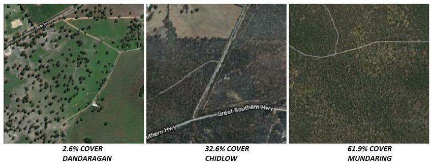
Agriculture 2020, 10, 118 3 of 17
2. Materials and Methods
2.1. Honey Harvest Data
Honey harvest data used for this study were from the same dataset used by Campbell, Fearns [9].
The dataset is from two apiarists: one ‘commercial’ apiarist with ~700 hives and one ‘hobby’ apiarist
with ~50 hives. This consisted of harvest data from 2011 to 2018, across 16 apiary sites (with not all
apiary sites being used every year). Honey harvest data were reduced to the average weight of honey
harvested per hive, per year, per apiary site (see Table 1). The data were also classified by this measure
as to whether the harvest was a ‘poor year’ (40 kg honey per hive).
Table 1. Summary of honey harvest data by site and year.
Site 2011 2012 2013 2014 2015 2016 2017 2018
101 N/A N/A N/A N/A 39.3 20.3 12.5 35.0
102 N/A N/A N/A N/A 36.3 0.0 4.0 30.0
103 N/A N/A N/A N/A N/A 6.0 10.0 28.1
201 Not used Not used 49.6 Not used 52.2 Not used Not used Not used
202 Not used Not used 65.6 Not used 45.5 Not used Not used Not used
204 16.1 Not used 71.0 Not used Not used Not used 26.8 40.2
205 0.0 Not used Not used Not used 48.2 Not used 13.4 38.8
206 Not used 0.0 18.8 Not used 29.5 Not used Not used 16.1
207 Not used 0.0 18.8 Not used 29.5 Not used Not used 16.1
208 Not used 8.0 16.1 16.1 12.1 Not used Not used 16.1
209 Not used Not used 18.8 Not used 20.1 Not used Not used 16.1
210 Not used Not used 56.3 Not used 67.0 Not used Not used Not used
211 Not used Not used 49.6 Not used 52.2 Not used Not used Not used
212 8.9 Not used 42.9 Not used 32.1 Not used 11.6 26.8
213 Not used 17.1 Not used Not used Not used Not used 44.2 Not used
Red = ‘poor year’ (40 kg per hive).
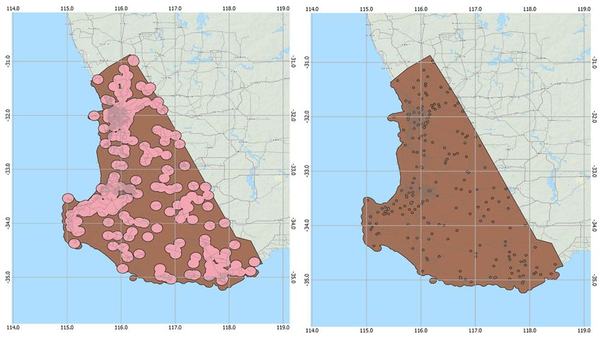
While most apiary sites were within 65 km of the capital city of Perth (Western Australia, −31.95
latitude 115.86 longitude), sites extended from as far north as Dandaragan (140 km north of Perth,
−30.66 latitude 115.70 longitude) to as far south as Boyup Brook (230 km south-east of Perth, −33.83
latitude 116.38 longitude). The locations of the apiary sites are shown in Figure 2. All sites experience a
warm temperate climate zone [10] and fall within the highly biodiverse South West Australian Floristic
Region [11]. While all sites are within the same broad climatic region, the geographic extent of the sites
means there is a range of annual weather trends within the study area, with the sites north of Perth
being hotter and drier and the site south of Perth being cooler and drier (further inland than Perth).
The mean annual and summer weather statistics for the three main areas are summarised in Table 2.
Table 2. Summary of key summary weather data for the three regions where sites are located.
ANNUAL SUMMER (DECEMBER–FEBRUARY)
REGION Mean Max. Mean Max.
Rainfall Rainfall
Temperature Temperature
Dandaragan (north of Perth) 25.9 ◦ C 484.5 mm 33.8 ◦ C 32.4 mm
Mundaring (Perth Hills) 22.6 ◦ C 1069 mm 29.7 ◦ C 49.3 mm
Boyup Brook (south of Perth) 22.4 ◦ C 649.1 mm 29.0 ◦ C 44.7 mm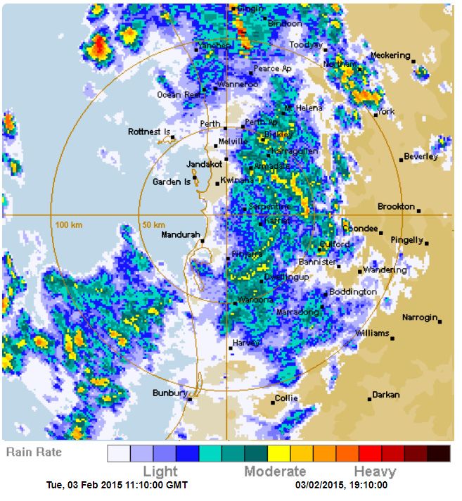
Agriculture 2020, 10, 118 4 of 17
Agriculture 2020, 10, x FOR PEER REVIEW 4 of 17
Agriculture 2020, 10, x FOR PEER REVIEW 4 of 17
Figure
Figure Apiary
2. 2. Apiarysite
sitelocations
locationsindicated
indicated by
by yellow markers.Site
yellow markers. Sitelabels
labelscorrespond
correspondto to those
those listed
listed in in
Table 1. 1.
Table Coordinates
Coordinatesare areininWorld
WorldGeodetic
GeodeticSystem
System 1984
1984 (WGS84).
(WGS84).
Figure 2. Apiary site locations indicated by yellow markers. Site labels correspond to those listed in
There was1. also
Table Coordinates
a largeare in World
range Geodetictree
of mature System 1984 (WGS84).
canopy cover across the sites. Using the vegetation
There was also a large range of mature tree canopy cover across the sites. Using the vegetation
structure
structure products
products produced
produced by
by Auscover
Auscover [12] inin combination
combinationwith with theheight
height range of of mature,
There was also a large range of mature [12]
tree canopy cover across thethe
sites. Usingrange mature,
the vegetation
flowering
flowering Corymbia
structure Corymbia
products calophylla
calophylla
produced(marri)
(marri) trees
trees of
by Auscover of 10–40
[12] inmmcombination
[13],the
[13], thepercentage
percentage ofmature
mature
with theofheight canopy
canopy
range cover
cover
of mature, forfor
thethe
apiary
flowering Corymbia calophylla (marri) trees of 10–40 m [13], the percentage of mature canopy cover for(for a
apiary sites ranges
sites ranges from
from as low
as low as
as2.6%
2.6% (for
(for aafarm
farm site
site near
near Dandaragan) to
to as
as high
high as
as 61.9%
61.9% (for
a forest
forest site
the sitethe
in
apiary in theranges
Beelu
sites Beelu National
National
from lowPark,
asPark, near
as near
2.6% (forMundaring)
Mundaring)
a farm sitewith with a median
a median
near mature
mature
Dandaragan) canopy
to ascanopy
high ascovercover
61.9% of of
(for32.6%.
32.6%.
Examples Examples
of site
a forest these of these
in canopy
the Beelu canopy
cover cover
extents
National extents
arenear
Park, shownare shown in
in Figurewith
Mundaring) Figure 3.
3. a median mature canopy cover of
32.6%. Examples of these canopy cover extents are shown in Figure 3.
Figure
Figure Examples
3. 3. Examples ofofthe minimum, median and maximum
maximummature
maturecanopy
canopycover
cover across the apiary
Figure 3. Examples ofthe
theminimum,
minimum,median
median and
and maximum mature canopy cover across
across the
the apiary
apiary
sites (images
sites (images
sites are
(images all
areare 1 km
allall
1 km × 1 km
1 km× ×1 1km extent).
kmextent).
extent).
2.2.2.2.
Temperature,
Temperature,
Rainfall
Rainfall
and Solar Exposure Datasets
2.2. Temperature, Rainfalland
andSolar
SolarExposure
ExposureDatasets
Datasets
These
These standard
These standard
standardmeteorological
meteorological datasets
datasetswere
meteorologicaldatasets were retrieved
were retrieved fromthe
from
retrieved from the
the Bureau
Bureau
Bureau of Meteorology
ofofMeteorology
Meteorology (BOM)’s
(BOM)’s
(BOM)’s
Australian
Australian Data
Australian Archive
Data
Data Archive for for
Archive Meteorology
forMeteorology
Meteorology(ADAM),
(ADAM),
(ADAM), a database
a database
databasethatthat
holds
that weather
holds
holds observations
weather
weather observationsdating
observations
back to the
dating mid-1800s
back to the for some
mid-1800s sites
for
dating back to the mid-1800s for some sites [14].[14].
some Daily
sites weather
[14]. Daily observations
weather stored
observations within
stored ADAM
within
weather observations stored within ADAM are
ADAM readily
accessible
areare online
readily
readily via BOM’s
accessible
accessible online
online Climate
viaBOM’s
via Data
BOM’s Online
Climate
Climate Data
Dataportal
Online
Online[15]. Weather
portal
portal [15]. stations
[15].Weather
Weather managed
stations by BOM
managed
stations managed
by BOM
arebyinstalled
BOM are are installed
andinstalled
operatedand and operated
to consistent
operated to to consistent
standards
consistent standards
[16], providing
standards [16], providing
a high
[16], a high
degree aofhigh
providing degree
degreeofwhen
confidence of
confidence
comparing
confidence data when
when betweencomparing
comparing data
yearsdata between
andbetween years and
sites. years and sites. sites.
While the individual weather station measurements have a high degree of confidence, weather
stations in the2020,
Agriculture study
10, x;area arePEER
doi: FOR widely
Agriculture 2020, 10, x; doi: FOR PEER REVIEW
spaced, with up to 38.9 km between
REVIEW apiary sites and the nearest
www.mdpi.com/journal/agriculture
www.mdpi.com/journal/agriculture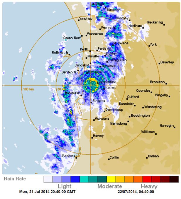
Agriculture 2020, 10, 118                                                                                                   5 of 17

weather station (Table 3). With the majority of the surveyed extent of the marri trees covering
~84,000 km2 [3], only ~11,000 km2 (or 13% of this area) has a temperature station within 10 km. This is
shown spatially in Figure 4. The relatively sparse weather station network means that the extrapolation
of temperature data to apiary sites may introduce some errors. Additionally, while a 10 km buffer from
the rainfall recording stations covers 50% of the surveyed extent of marri trees, the spatial extent of
rainfall events, particularly summer thunderstorms, can be much less.

      Table 3. Distances between apiary sites and weather stations Bureau of Meteorology (BOM) weather
      station locations retrieved from [17].

                             Nearest Temperature                              Nearest Rainfall
          Apiary Site                                   Distance (km)                                 Distance (km)
                                   Station                                        Station
              101              PEARCE RAAF                    12.3              MARBLING                    3.7
              102                 BICKLEY                     10.5             MAIDA VALE                   5.2
              103                 BICKLEY                      9.7             ROLEYSTONE                   3.6
              201                 BICKLEY                      6.2               BICKLEY                    6.2
              202                 BICKLEY                     23.9              CHIDLOW                     5.5
              203                 BICKLEY                     24.5             WOOROLOO                     4.7
                                                                                  LAKE
              204                   BICKLEY                   19.3                                          1.8
                                                                             LESCHENAULTIA
              205                 BICKLEY                     27.0             WOOROLOO                     6.9
                               BADGINGARRA
              206                                             38.9               CHELSEA                    4.9
                               RESEARCH STN
                               BADGINGARRA
              207                                             33.3               TAMBREY                    2.4
                               RESEARCH STN
                                 LANCELIN                                     DANDARAGAN
              208                                             34.6                                          3.2
                                 (DEFENCE)                                        WEST
                                 LANCELIN                                     DANDARAGAN
              209                                             37.9                                          1.2
                                 (DEFENCE)                                        WEST
              210                 BICKLEY                      1.2               BICKLEY                    1.2
              211                 BICKLEY                      4.8               BICKLEY                    4.8
              212                 BICKLEY                     20.1              CHIDLOW                     0.1
                                BRIDGETOWN
              213                                             29.9            BOYUP BROOK                   10.0
                                COMPARISON
      Shaded cells indicate either temperature stations further than 10 km from the apiary site or rainfall stations more
      than 2 km from the apiary site.
         Agriculture 2020, 10, x FOR PEER REVIEW                                                                  6 of 17

      Figure 4. Coverage
             Figure        of Bureau
                    4. Coverage        of Meteorology
                                of Bureau  of Meteorology(BOM)      rainfall
                                                           (BOM) rainfall andand  temperature
                                                                               temperature     weather
                                                                                           weather stationsstations
                                                                                                             over   over
             the geographic extent of marri trees. Coordinates are in
      the geographic extent of marri trees. Coordinates are in WGS84. WGS84.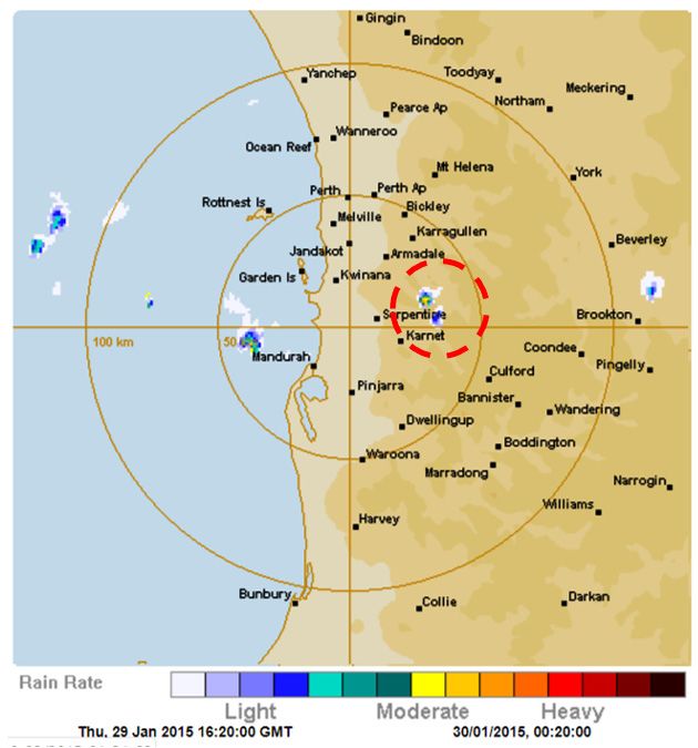
Agriculture 2020, 10, 118                                                                                              6 of 17

      An example of the rainfall from such a storm event is shown in Figure 5. The main storm feature
is approximately 18 km across its long axis but the more intense central area, where rainfall may be as
high as 200 mm/h in this case, is just over 2 km across. Reducing the buffer around the BOM rainfall
stations to 2 km means that only 3.1% of the marri spatial extent is sufficiently close to a rainfall station
to reliably detect these isolated, yet intense, summer rain events. With summer rainfall being one of
the key  indicators of marri honey harvest weight [9], this lack of coverage may limit the ability of the
      Figure 4. Coverage of Bureau of Meteorology (BOM) rainfall and temperature weather stations over
BOMthe rainfall data to reliably classify or predict honey harvest weight.
         geographic extent of marri trees. Coordinates are in WGS84.

                      (a) summer storm                                            (b) winter cold front

      Figure 5.
              5. Examples
                 Examplesofofrainfall
                                rainfallevents
                                          events  from
                                               from   thethe  Perth
                                                          Perth      region
                                                                region       viewed
                                                                        viewed   in theinBureau
                                                                                          the Bureau    of Meteorology
                                                                                                  of Meteorology  (BOM)
      (BOM)   rain
      rain radar  forradar
                      Perthfor
                            [18]Perth
                                 for (a)[18] for (a) and
                                         a localised   a localised  and intense
                                                           intense summer     stormsummer
                                                                                     event instorm    event
                                                                                                January      in January
                                                                                                         (highlighted in
      (highlighted
      red), and (b) in
                     thered),
                         stormand (b) of
                                front thea storm
                                            winterfront  of a winterinthunderstorm
                                                    thunderstorm       July.           in July.

      The distances between
2.3. Satellite-Derived Data  the apiary sites where the honey harvest data is from and the nearest
weather stations are provided in Table 3, with temperature stations more than 10 km away and rainfall
      All other input datasets for modelling were derived from the Moderate Resolution Imaging
stations greater than 2 km away highlighted. A total of 75% of the apiary sites are more than 10 km
Spectrometer (MODIS) sensor which is carried on the Terra and Aqua satellites [19], with data
from the nearest temperature station and 75% of the apiary sites are more than 2 km from the nearest
retrieved from the Application for Extracting and Exploring Analysis Ready Samples (AppEEARS)
rainfall station. Only one apiary site was within both 10 km of a temperature station and 2 km of a
online portal [20]. A summary of the scientific basis for the creation of these datasets follows below.
rainfall station.

2.3. Satellite-Derived
Agriculture                Data
            2020, 10, x; doi: FOR PEER REVIEW                                            www.mdpi.com/journal/agriculture

     All other input datasets for modelling were derived from the Moderate Resolution Imaging
Spectrometer (MODIS) sensor which is carried on the Terra and Aqua satellites [19], with data retrieved
from the Application for Extracting and Exploring Analysis Ready Samples (AppEEARS) online
portal [20]. A summary of the scientific basis for the creation of these datasets follows below. All
datasets were retrieved from the AppEEARS portal at a pixel size of 1000 × 1000 m, from the pixel
in which the apiary site is located. Retrieving data from coincident pixels meant that the subsequent
integration of the data into a single database was a straightforward process. This pixel size was selected
based on the typical forage range for honeybees with moderate nectar availability being 1–2 km [21].
This spatial resolution scale is also in line with studies elsewhere in the world investigating links
between honeybee foraging and satellite data, such as eastern Australia [6] and Europe [22]. These
studies concluded that, due to the foraging distances, the larger pixels of MODIS datasets were a more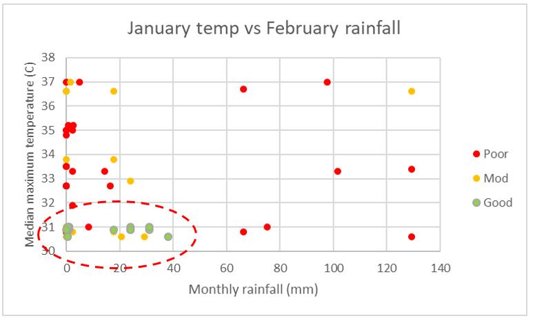
Agriculture 2020, 10, 118                                                                            7 of 17

accurate representation of the foraging conditions for a given apiary site than data from sensors with a
higher spatial resolution.
      All satellite derived data sets were filtered using the quality control channel contained in the
AppEEARS download files. The particulars of the quality control parameters for each dataset can be
found in the references provided in the following paragraphs. The quality control filter was set to only
allow the highest quality data through into the machine learning algorithm input dataset.
      The Gross Primary Production (GPP) MODIS-derived product was developed by Running
and Nemani [23], based on the theory that productivity of crops with sufficient water and nutrient
availability is linearly related to the amount of absorbed solar radiation and the efficiency of its
use [24]. The MOD17 data product [25] used for this study incorporates the vegetation conversion
efficiency factor (ε), as well as the effect of water stress and cold conditions on this conversion factor.
Ground-based validation of the MOD17 data by Turner and Ritts [26] found that MOD17 GPP is
responsive to general trends associated with local climate and land use, but tended to overestimate
GPP in low productivity areas and underestimate GPP in high production areas.
      The MOD16A2 Net Evapotranspiration data product [27] is based on the retrieval of key parameters
of the Penman–Monteith evapotranspiration formula from MODIS data [28]. A reliability study of this
data product in dry, heterogenous forests against ground measurements yielded a strong correlation of
r2 = 0.82 [29], indicating the high overall reliability of the product.
      The Normalized Difference Vegetation Index (NDVI) and Enhanced Vegetation Index (EVI) were
both retrieved from the MOD13Q1 data product [30]. NDVI has been found to be strongly related to
leaf chlorophyll content, whereas EVI is more indicative of canopy structural variations, including leaf
area index (LAI) [31].
      The Marri Flowering Index (MFI), developed by Campbell and Fearns [32], was designed for
direct detection of marri flowers from MODIS data, based on an analysis of spectroradiometer surveys
of this particular species. While the MFI has proven to be an effective index for classifying the marri
honey harvest weight for some apiary sites with a high proportion of canopy cover [32], it appears to
be less reliable across multiple apiary sites and years [9].
      The Normalised Difference Water Index (NWDI) [33] is sensitive to changes in the liquid water
content of vegetation canopies. This is a proven metric for vegetation water stress [34], which may
impact bud development and nectar production.

2.4. Classification and Regression Tree Analysis
     Classification and regression trees [35] are machine learning methods commonly used to build
predictive models from input data [36]. Both methods partition the input dataset into smaller subsets
and perform a simple prediction for each subset. By repeating this process over the entire dataset and
combining the simple predictions together, a ‘tree’ type classification or regression structure is made.
Classification trees are used for predictive models based on discreet classes or values, while regression
trees are used for continuous variables or ranges.
     To develop a predictive model, we tested two kinds of regression and classification approaches.
Boosted Regression Trees (BRTs) are versatile, tree-based regression methods that can handle input
features of different data types, while handling complex nonlinear relationships as well as interaction
effects between the input features [37]. Random Forest trees have become popular in recent years for
remote sensing and ecological applications due to their ability to handle both high data dimensionality
and multicollinearity, which are common in multi-spectral remote sensing data, and the fact that they
are both fast and insensitive to overfitting [38]. The Scikit-learn code for Python was used for the
analysis [39], with the GradientBoostingRegressor, GradientBoostingClassifier, RandomForestRegressor and
RandomForestClassifier functions initially used to assess which approach resulted in the most accurate
predictive model.
Agriculture 2020, 10, 118 8 of 17
2.5. Results
Input data were retrieved from several different sources for periods both preceding and during
the main honey flow period for marri trees (February). The sources, periods and abbreviations used
hereafter for these data are provided in Table 4. In total, a multidimensional database of 115 input
features was created from the data summarised in Table 4.
Table 4. Summary of features used in the regression tree analysis.
Feature Months Used Data Source
Median maximum monthly temperature during flowering
MaT: Median maximum monthly
(MaTD) to the median maximum monthly temperature for
temperature (◦ C)
the 11 months preceding flowering (MaT11)
Median minimum monthly temperature during flowering
MiT: Median minimum monthly
(MiTD) to the median minimum monthly temperature for
temperature (◦ C)
the 11 months preceding flowering (MiT11)
Total number of days above 40 ◦ C during flowering (T40D)
T40: Number of days above 40 ◦ C to total number of days above 40 ◦ C for the 6 months Australian Data Archive for
preceding flowering (T406) Meteorology (BOM) [15]
Total number of days below 25 ◦ C during flowering (T25D)
T25: Number of days below 25 ◦ C to the total number of days below 25 ◦ C for the 6 months
preceding flowering (T256)
Total rainfall during flowering (RD) to the total rainfall
R: Monthly rainfall (mm)
during the 11 months preceding flowering (R11)
Mean solar exposure during flowering (SRad) to the mean
SRad: Nett mean monthly Solar
solar exposure for the 11 months preceding flowering
Exposure (MJ/m2 )
(SRad11)
Application for Extracting and
Gross Primary Productivity from 1 month prior to
GPP: Gross Primary Productivity Exploring Analysis Ready
flowering (GPP1) to the Gross Primary Productivity from
(kgCm2 ) Samples (A%%EEARS)
the 11 months prior to flowering (GPP11)
[20]-MOD17A2H product
Net Photosynthesis from 1 month prior to flowering
PSN: Net Photosynthesis (PSN1) to the Net Photosynthesis from 11 months prior to A%%EEARS—MOD17A2H product
flowering (PSN11)
Evapotranspiration from 1 month prior to flowering (ET1)
ET: Evapotranspiration
to the Evapotranspiration from the 11 months prior to A%%EEARS—MOD16A2 product
(kg/m2 /day)
flowering (ET11)
Average Latent Heat Flux from 1 month prior to flowering
LE: Average Latent Heat Flux
(LE1) to the Average Latent Heat Flux from the 11 months A%%EEARS—MOD16A2 product
(J/m2 /day)
prior to flowering (LE11)
Total Potential Evapotranspiration from 1 month prior to
PET: Total Potential
flowering (PET1) to the Total Potential Evapotranspiration A%%EEARS—MOD16A2 product
Evapotranspiration (kg/m2 /day)
from the 11 months prior to flowering (PET11)
Average Potential Latent Heat Flux from 1 month prior to
PLE: Average Potential Latent
flowering (PLE1) to the Average Potential Latent Heat Flux A%%EEARS—MOD16A2 product
Heat Flux (J/m2 /day)
from the 11 months prior to flowering (PLE11)
Average NDVI from 1 month prior to flowering
NDVIA: Average Normalized
(NDVIAv1) to the average NDVI for the 11 months prior to A%%EEARS—MOD13A1 product
Difference Vegetation Index
flowering (NDVIAv11)
Maximum NDVI from 1 month prior to flowering
NDVIM: Maximum Normalized
(NDVIMx1) to the maximum NDVI for the 11 months A%%EEARS—MOD13A1 product
Difference Vegetation Index
prior to flowering (NDVIMx11)
Average EVI from 1 month prior to flowering (EVIAv1) to
EVIA: Average Enhanced
the average EVI for the 11 months prior to flowering A%%EEARS—MOD13A1 product
Vegetation Index
(EVIAv11)
Maximum EVI from 1 month prior to flowering (EVIMx1)
EVIM: Maximum Enhanced
to the maximum EVI for the 11 months prior to flowering A%%EEARS—MOD13A1 product
Vegetation Index
(EVIMx11)
AppEEARS—derived from
MFI: Marri Flowering Index Maximum Marri Flowering Index (MFI) value for February
MODOCGA product
Average NDWI from 1 month prior to flowering
NDWI: Normalized Difference AppEEARS—derived from
(NDWIAv1) to the average NDWI for the 11 months prior
Water Index MOD09A1 product
to flowering (NDWIAv11)Agriculture 2020, 10, 118 9 of 17
To assess the predictive accuracy of each algorithm, both the regression and classifier functions
for the gradient boosted and Random Forest tree algorithms were run for all 115 input features, with
an increasing number of trees in the model. No complexity limit was given due to the relatively small
size of the dataset and the resulting short run time. The output from this testing (see Table 5) shows
that the Random Forest functions worked better for the classification approach, based on the ‘poor
year’, ‘moderate year’ and ‘good year’ ratings, and the Gradient Boosted functions worked better for
predicting the honey harvest weights via the regression model.
Table 5. Summary of predictive errors for different sized Random Forests.
RANDOM FOREST TREES GRADIENT BOOSTED TREES
Number of
Algorithm Honey Honey Honey Honey Honey Honey
Trees Weight Weight Class Weight Weight Class
Regression Classification Classification Regression Classification Classification
5 11.68 kg 25% 50% 13.49 kg 50% 42%
10 13.63 kg 25% 50% 11.38 kg 25% 42%
20 12.46 kg 25% 42% 10.42 kg 18% 42%
50 11.48 kg 25% 42% 10.55 kg 18% 42%
100 11.31 kg 25% 33% 10.35 kg 18% 42%
200 11.63 kg 25% 33% 10.33 kg 18% 42%
500 11.56 kg 25% 33% 10.33 kg 18% 42%
1000 11.29 kg 25% 33% 10.33 kg 18% 42%
5000 11.43 kg 25% 33% 10.33 kg 18% 42%
Note that the ‘Honey weight classification’ is performed by doing the ‘Honey weight regression’, then classifying the
predicted honey weight into the appropriate class of ‘poor year’, ‘moderate year’, or ‘good year’. The ‘Honey class
classification’ output is provided by the relevant ‘Classifier’ function. The lowest predictive errors are highlighted
in green.
The lowest predictive errors came from the use of Gradient Boosted Regression (GBR), with a
mean average error of +/− 10.3 kg for the weight, with this weight being in the correct class 82% of
the time.
The partial dependence plots for the 10 features with the highest feature importance from the
full feature input model are shown in Figure 6. These plots show that the model predictions have the
highest dependence on the mean maximum temperature for October–January (MaT4), with mean
maximum temperatures below 27 ◦ C having a strong positive relationship and mean maximum
temperatures above 27 ◦ C having a negative relationship. There are also strong relationships with
Gross Primary Production from the 11 months preceding the flowering period (GPP11), with low GPP
associated with lower honey production, and a higher evapotranspiration for January (ET1) having a
positive relationship with higher honey production.Agriculture 2020, 10, 118 10 of 17
Agriculture 2020, 10, x FOR PEER REVIEW 10 of 17
(a) (b)
(c) (d)
(e) (f)
(g) (h)
(i) (j)
Figure
Figure 6. 6. Partialdependence
Partial dependenceplotsplots for
for 10
10 most
most important
importantfeatures
features(Gradient
(GradientBoosted
BoostedRegression).
Regression).
Refer
Refer to Table
to Table 4 for
4 for thethe featureacronym
feature acronymdefinitions.
definitions. (a)
(a) Average
Averagemaximum
maximumtemperature
temperature forfor
October
October
to January
to January (b)(b) evapotranspirationfor
evapotranspiration forJanuary
January (c)
(c) Gross
Gross Primary
PrimaryProductivity
Productivityfrom
fromMarch to to
March January
January
(d) Net Photosynthesis For March to January (e) Solar Radiation for January (f)
(d) Net Photosynthesis For March to January (e) Solar Radiation for January (f) Total Potential Total Potential
Evapotranspiration For August to January (g) rainfall from December to January (h) average
Evapotranspiration For August to January (g) rainfall from December to January (h) average maximum
maximum temperature in January (i) maximum Enhanced Vegetation Index from December to
temperature in January (i) maximum Enhanced Vegetation Index from December to January (j) rainfall
January (j) rainfall from August to January.
from August to January.
Agriculture 2020, 10, x; doi: FOR PEER REVIEW www.mdpi.com/journal/agricultureAgriculture 2020, 10, 118 11 of 17
In order to determine whether the dimensionality of the input features could be reduced without
compromising the predictive accuracy of our models, the GBR function was run multiple times with
fewer input features for each run. The selection of input features for each run was on the basis of the
highest feature importance from the preceding model. Table 6 shows the VIs and predictive errors for
this process. The MaT4 feature is clearly the most important input, with a VI of 37.7% even when all
115 features are used in the regression modelling. This is followed by ET1 and GPP, both at below
10% when all feature inputs are used. The columns highlighted in green show the models with the
lowest error, by class (five input features) and by weight (two input features). These reduced input
feature models both have slightly higher honey weight prediction errors than the full feature model
(increased error of 0.52 kg versus a honey harvest range of 0.0 kg to 71.0 kg in the training and testing
datasets). If this simplified approach were to be applied to larger datasets for the prediction of honey
harvest weight, a significantly smaller number of feature inputs can be used, with a minimal reduction
in predictive accuracy, reducing the size of the multidimensional dataset required.
Table 6. Gradient Boosted Regression errors and feature importance (import.) for differing number of
input features.
# Features All 10 8 6 5 4 3 2 1
Honey weight 10.33 kg 11.75 kg 9.56 kg 12.87 kg 10.85 kg 11.61 kg 10.91% 10.42 kg 11.72 kg
Honey class.
17% 17% 17% 25% 8% 17% 17% 17% 25%
(1–3)
Honey class.
0% 0% 0% 0% 0% 0% 0% 0% 0%
(1–2)
MaT4 import. 37.7% 30.7% 31.7% 45.7% 48.9% 56.8% 57.0% 63.2% 100%
ET1 import. 7.9% 18.6% 15.4% 25.0% 26.3% 29.3% 31.0% 36.8%
GPP11 import. 5.9% 11.3% 14.4% 10.0% 11.1% 8.4% 12.0%
NSP11 import. 5.7% 9.8% 12.5% 7.5% 7.3% 5.5%
SRad1 import. 4.0% 8.0% 8.8% 6.0% 6.5%
PET6 import. 3.7% 6.2% 6.6% 5.8%
R2 import. 3.7% 5.4% 6.1%
MaT1 import. 3.2% 4.6% 4.6%
EVIMx2 import. 2.8% 3.9%
R6 import. 2.7% 1.6%
The models with the lowest errors are highlighted in green. Gray cells are where the input features were not used in
the classification algorithm.
The ‘Honey class. (1–2)’ row in Table 6 is calculated by classifying the predicted honey weight
as either ‘good year’ or ‘below good year’, based on the high degree of clustering found with key
weather and satellite inputs for ‘good years’ by Campbell and Fearns [9]. This tight clustering for
‘good years’, and the 0% error in the predictive regression classification, means that for this dataset
the ‘good year’ prediction is both an accurate and a robust model. While this cannot assist apiarists
with preparation for ‘poor years’, when their bees can sometimes starve due to the lack of nectar,
the apiarists can prepare for a ‘good year’ in advance and therefore increase the honey production,
compared with being unprepared for a ‘good year’ and having insufficient hives or other equipment
to facilitate efficient use of the abundant resource.
Although the predictive regression model developed solely from the MaT4 and ET1 features has a
relatively low error and is shown to be quite robust at predicting harvests that are ‘good years’, both
input features require data from the month immediately preceding the honey flow. If the predictive
model developed here was used operationally by beekeepers to adaptively manage their beehives, this
timing of the key input data would limit the time available for apiarists to prepare for a ‘good year’. To
determine whether a predictive model could be generated with a longer lead time into the honey flow,
mean maximum temperatures for the individual months from October to January were also tested
in the GBR, as well as combinations of these months. The VIs from this process are summarised in
Table 7. While the original MaT4 and ET1 features retained a high importance, MaT3 (mean maximum
temperature for November) was also assessed as a key feature input, based on a visual assessment ofAgriculture 2020, 10, x FOR PEER REVIEW 12 of 17
process are summarised in Table 7. While the original MaT4 and ET1 features retained a high
Agriculture 2020, 10, 118 12 of 17
importance, MaT3 (mean maximum temperature for November) was also assessed as a key feature
input, based on a visual assessment of the clustering of each feature versus honey harvest weight (see
Figure 7). While
the clustering the model
of each featuredoes not honey
versus produce the lowest
harvest errors,
weight it is nonetheless
(see Figure 7). While thea reliable
modelpredictor
does not
(particularly
produce for ‘good
the lowest years’
errors, it isversus non-good
nonetheless years).predictor
a reliable The lower accuracy offor
(particularly the‘good
prediction
years’isversus
offset
non-good years). The lower accuracy of the prediction is offset by the lead time to the honey flow;early
by the lead time to the honey flow; with honey flow generally starting in late January to with
February
honey flow[32], having astarting
generally strong in indicator of an upcoming
late January good harvest
to early February by the aend
[32], having of November
strong indicator gives
of an
apiarists approximately
upcoming good harvest by two months
the end of to prepare for
November theapiarists
gives predicted conditions. two months to prepare
approximately
for the predicted conditions.
Table 7. Gradient Boosted Regression errors and the feature importance of mean temperatures 1–4
months
Table 7. before flowering
Gradient Boostedand evapotranspiration
Regression errors and1the
month before
feature flowering.
importance of mean temperatures 1–4
months before flowering and
# Features 10 evapotranspiration
8 6 1 month 4before flowering.
3 MaT3 + ET1 MaT3
Honey
# Featuresweight 1010.09 kg 810.34 kg 9.64
6 kg 11.16
4 kg 10.44
3 kg 8.92+kgET1
MaT3 11.72 kg
MaT3
Honey class.
Honey weight (1–3)
10.09 kg17% 25%
10.34 kg 17%
9.64 kg 25%
11.16 kg 17%
10.44 kg 17%kg
8.92 25%
11.72 kg
Honey class.
Honey class. (1–3)(1–2) 17% 0% 25% 0% 17% 0% 25% 0% 0%
17% 0%
17% 0%
25%
HoneyET1
class. (1–2)
import. 0% 28.3% 0% 28.3% 0%28.4% 0%
35.1% 0%
36.8% 0%
38.1% 0%
ET1 import.
MaT 1–4 import. 28.3%24.5% 28.3%
35.1% 28.4%
33.8% 35.1%
17.1% 36.8%
38.3% 38.1%
MaT 1–4 import. 24.5% 35.1% 33.8% 17.1% 38.3%
MaT 2–3 import. 24.1% 13.9% 16.9% 37.5% 24.9%
MaT 2–3 import. 24.1% 13.9% 16.9% 37.5% 24.9%
MaTMaT 2 import. 5.7%5.7% 8.2%8.2% 8.9%
2 import. 8.9% 10.4% 10.4%
MaTMaT
3–4 3–4 import. 3.2%3.2% 3.4%3.4% 3.2%
import. 3.2%
MaTMaT 1 import. 8.9%8.9% 8.8%8.8% 8.9%
1 import. 8.9%
MaT 2–4 2–4
MaT import.
import. 1.2%1.2% 1.8%1.8%
MaT 1–2 import.
MaT 1–2 import. 3.6%3.6% 0.6%0.6%
MaT 3 import. 0.4% 61.9% 100%
MaT 3 import. 0.2%0.4%
MaT 4 import.
61.9% 100%
MaT 4 import. 0.2%
The models with the lowest errors are highlighted in green. Gray cells are where the input features were not used in
Thethe
models with the
classification lowest errors are highlighted in green. Gray cells are where the input features were not
algorithm.
used in the classification algorithm
Figure 7. Mean monthly maximum temperature for November (MaT3) versus honey harvest
Figure 7. Mean monthly maximum temperature for November (MaT3) versus honey harvest weight.
weight.
3. Discussion
3. Discussion
From the regression tree analysis performed in this study, there are a range of different factors
From the the
that influence regression tree analysis
honey harvest performed
of marri trees andin this
the study, there
timeframe are aofrange
of some these of different
factors (e.g.,factors
Gross
that influence
Primary the honeycan
Productivity) harvest
be as of marriastrees
much andbefore
a year the timeframe
the honeyofflow
somestarts.
of these factorsthe
Despite (e.g., Gross
range of
Primary Productivity)
available input variablescanthat
be we
as much as a we
explored, year before
found thatthethe
honey flow
inputs starts.
to the Despitemodel
predictive the range of
can be
available input variables that we explored, we found that the inputs to the predictive
reduced significantly with a minimal reduction in the accuracy of the predictive model. The mean model can be
reduced significantly
maximum temperaturewith
forathe
minimal reduction
few months in the accuracy
preceding honey flowof the predictive
(November to model.
January)Theandmean
the
evapotranspiration in the month before honey flow (January) were found to describe the majority of
Agriculture 2020, 10, x; doi: FOR PEER REVIEW www.mdpi.com/journal/agricultureAgriculture 2020, 10, x FOR PEER REVIEW 13 of 17
Agriculture 2020, 10, 118 13 of 17
maximum temperature for the few months preceding honey flow (November to January) and the
evapotranspiration in the month before honey flow (January) were found to describe the majority of
the variability
the variability in in honey
honey harvest
harvest weight
weight almost
almost as asaccurately
accurately asasthe
thefull
fullmultidimensional
multidimensional dataset
dataset ofof
115input
115 inputfeatures.
features.
The potential
The potentiallimitations
limitationsin inthe
the accuracy
accuracyof of the
the weather
weather station
station data
data available
availablefrom
fromBOM,
BOM,due duetoto
thesparsity
the sparsityof of stations
stations across
across the extent
the extent of marri oftrees
marri treestheversus
versus spatialthe spatial ofvariability
variability of the
the observations,
observations,
may mean thatmay somemean that some between
relationships relationships marri between marri honeyand
honey production production
weather and mayweather may
not be fully
not be fully captured in the existing database. The sparse nature of rainfall
captured in the existing database. The sparse nature of rainfall stations compared to the localised stations compared to the
localised
nature nature ofrainfall
of summer summer rainfall
events events
means that means that the
the influence ofinfluence
rainfall inof rainfall in
particular particular
may may
have been have
poorly
been poorly characterised in our input dataset. Unfortunately, due to this sparsity
characterised in our input dataset. Unfortunately, due to this sparsity of rainfall stations, excluding of rainfall stations,
excluding
apiary sitesapiary
from the sites from the
database thatdatabase that have stations
have temperature temperature
more stations
than 10 km moreawaythan 10 km
and/or away
rainfall
and/or rainfall
stations more than stations more would
2 km away than 2result
km away in only would result site
one apiary in only
in the one apiary with
database site in the database
honey harvests
with two
from honey of harvests
the study from twoThis
years. of theis study years. data
insufficient This for
is insufficient
the developmentdata forofthe development
a predictive of a
model,
predictive model,
particularly as bothparticularly
of these years as are
both of these
‘good years’ years
(>40are ‘good
kg of marriyears’
honey (> per
40 kg of marri honey per
hive).
hive).Rainfall immediately preceding and during the flowering period is one of the key factors in harvest
qualityRainfall immediately
(see Figure preceding
8), with heavy summer andrainfall
duringeventsthe flowering period
after flowering is one of the
commences key knocking
actually factors in
harvest and
stamen, quality (see Figure
sometimes 8), with
flowers, fromheavy summer
the trees [40].rainfall events after
This presents flowering
an issue commences
with the development actually
of a
knocking stamen, and sometimes flowers, from the trees [40]. This presents
predictive model as, even with good conditions in the lead up to the peak flowering period, a localised an issue with the
development
storm of a predictive
may downgrade model as,harvest
a prospective even with fromgood conditions
a ‘good year’ toinathe lead up year’
‘moderate to theorpeak flowering
even a ‘poor
period,
year’ in aa matter
localised storm may downgrade a prospective harvest from a ‘good year’ to a ‘moderate
of hours.
year’ or even a ‘poor year’ in a matter of hours.
Figure 8. Relationship between January temperature February rainfall and honey harvest (excerpt
Figure 8. Relationship between January temperature February rainfall and honey harvest (excerpt
from Campbell and Fearns [9]).
from Campbell and Fearns [9]).
Such a localised storm may have been the cause of the quality of some of the ‘moderate year’
Such a localised storm may have been the cause of the quality of some of the ‘moderate year’
harvests in the Perth Hills in 2015 being incorrectly classified as ‘good years’ by the predictive model;
harvests in the Perth Hills in 2015 being incorrectly classified as ‘good years’ by the predictive model;
the November mean maximum temperature was within the range for a good harvest that season, but
the November mean maximum temperature was within the range for a good harvest that season, but
three of the eight apiary sites only yielded a harvest that was a ‘moderate year’. Rainfall for all of the
three of the eight apiary sites only yielded a harvest that was a ‘moderate year’. Rainfall for all of the
apiary sites was below 40 mm for February (in the range 18.6–30.0 mm). The rainfall radar image from
apiary sites was below 40 mm for February (in the range 18.6–30.0 mm). The rainfall radar image
the main rainfall event at the start of the month, shown in Figure 9, contains localised patches of more
from the main rainfall event at the start of the month, shown in Figure 9, contains localised patches
intense rainfall (up to 80 mm/hr) that are under 2 km across. The presence of one of these localised
of more intense rainfall (up to 80 mm/hr) that are under 2 km across. The presence of one of these
higher intensity zones over an apiary site may well have increased the rainfall received by the site to
localised higher intensity zones over an apiary site may well have increased the rainfall received by
over 40 mm for the period, the upper limit for good harvests from the currently available data [9].
the site to over 40 mm for the period, the upper limit for good harvests from the currently available
data [9].
Agriculture 2020, 10, x; doi: FOR PEER REVIEW www.mdpi.com/journal/agricultureAgriculture 2020, 10, 118 14 of 17
Agriculture 2020, 10, x FOR PEER REVIEW 14 of 17
Figure 9.
Figure 9. Rainfall
Rainfall radar
radar map
map for
for min
min rainfall
rainfall event
event over
over the
the Perth
Perth Hills
Hills in
in early
early February
February 2015
2015 [18,41].
[18,41].
With marri
With marri honey
honey being
being thethe largest
largest annual
annual honey
honey harvest in Western
Western Australia
Australia [42],
[42], the
the highly
highly
specific conditions required for a good harvest may be less likely to occur with
specific conditions required for a good harvest may be less likely to occur with the projected climate the projected climate
modelsfor
models forthethe extent
extent to which
to which marrimarri trees occur.
trees occur. The Regional
The Regional Climate
Climate Model Model developed
developed for southwestfor
southwest
Western Westernby
Australia Australia
Andrys by andAndrys andassessed
Kala [42] Kala [42]projections
assessed projections
of both mean of both
andmean andweather
extreme extreme
weather
events events
over over the
the period fromperiod
2030from
to 20592030 to 2059
under under
a high a high greenhouse
greenhouse gas emissions gasscenario.
emissions scenario.
Compared
Compared
with historicwith historic
data from 1970data from
to 1999, 1970
mean to 1999,temperatures
maximum mean maximum temperatures
for spring and summer forare
spring and
projected
summer are projected to ◦
increase by between 0.5–2.0℃. With more than 80%
to increase by between 0.5–2.0 C. With more than 80% of the ‘good years’ occurring in seasons where of the ‘good years’
occurring
the in seasons
preceding Novemberwhere the preceding
mean maximumNovember
temperature mean maximum
is less than 24.0 ◦ C. As theis
temperature less than 24.0℃.
November mean
As the November
maximum temperaturemean formaximum
the Perth Hillstemperature
region is for the Perth
already ◦
at 25.0Hills region
C, the is already
probability at 25.0℃,
of this criteria the
for
probability of this criteria for a good harvest being met will likely decrease.
a good harvest being met will likely decrease. In addition, while the projections for summer rainfall In addition, while the
projections
vary for summer
considerably between rainfall
models, vary
theconsiderably between
models all predict thatmodels, the models
the intensity of summerall predict
rainfallthat the
events
intensity
will of summer
increase, rainfall
resulting events will
in an increase increase,
in the resulting
probability in an increase
of localised rainfallinevents
the probability
of sufficientof localised
intensity
rainfall
to reduceevents of sufficient
the harvest quality. intensity to reduce the harvest quality.
4.
4. Conclusions
The
The development
development of of aa multidimensional
multidimensional database
database with
with 115 factors that may influence the honey
production
production of of marri
marri trees
trees was
was subjected
subjected to to aa regression
regression tree
treeanalysis.
analysis. The
The GBR
GBR models
models achieved
achieved the the
highest
highest predictive accuracy when all features from the multi-dimensional dataset were used, with an
predictive accuracy when all features from the multi-dimensional dataset were used, with an
average
average error of +/−
error of 10.33 kg
+/− 10.33 kg for
for the
the weight,
weight, with
with the
the weight
weight being
being in the
the correct
correct class 82% of the time.
A
A similar
similarlevel
levelofofpredictive
predictiveaccuracy
accuracywaswas
achieved with with
achieved a revised GBR model
a revised GBR using
modelthe inputthe
using features
input
with the five highest values of feature importance. This regression model was able to
features with the five highest values of feature importance. This regression model was able to predict predict the honey
yield per hive
the honey yieldwith
perahive
mean average
with a mean error (MAE)
average of 10.85
error (MAE) kg of
and classify
10.85 kg andthe classify
harvest the
intoharvest
the correct
into
quality category
the correct qualitywith 92% accuracy.
category with 92% accuracy.
Analysis
Analysis ofof the
the predictive
predictive accuracy
accuracy of GBRs with different
different input
input features
features highlighted
highlighted that
that ‘good
‘good
years’
years’ could
could bebe predicted
predicted robustly
robustly compared
compared with with ‘moderate
‘moderate years’
years’ and
and ‘poor
‘poor years’
years’ (100%
(100% accuracy
accuracy
with
with only
only one
one oror two
two input
input features
features inin the
the models).
models). With mean maximummaximum temperature
temperature in in the
the months
months
leading
leading up
up to
to the
the marri
marri honey
honey flow
flow consistently
consistently rating
rating among
among thethe highest
highest importance
importance values,
values, testing
testing
the model with various combinations found that using the November mean maximum temperature
on as the only input feature into the GBR algorithm could predict the honey harvest weight per hive
Agriculture 2020, 10, x; doi: FOR PEER REVIEW www.mdpi.com/journal/agricultureAgriculture 2020, 10, 118 15 of 17
the model with various combinations found that using the November mean maximum temperature
on as the only input feature into the GBR algorithm could predict the honey harvest weight per hive
to an MAE of 11.72 kg, classify it into the correct class with 75% accuracy and predict a ‘good year’,
versus other types of year, to 100% accuracy. With the honey flow typically starting in February, giving
apiarists a reliable predictor of a good season two months ahead of time will allow them to prepare
their equipment, including establishing new hives, before the flow starts to improve the production in
years with good honey harvests.
In an operational setting, the accuracy of the prediction models may be restricted by the availability
of weather data, with less than 13% of the extent of marri trees having a temperature station within
10 km. Intense localised summer rainfall events also have an important role to play in making the model
more widely applicable. Only 3.1% of the marri areas have a rainfall station within 2 km. Access to more
spatially accurate weather data may be able to improve the regression model’s predictive accuracy.
With cooler weather and lower summer rainfall required for good marri honey harvests, the
climate projections for southwest Western Australia indicate that good harvests are likely to become
rarer in the future, with mean maximum temperatures and the intensity of summer rainfall both
projected to increase.
While this study has been focused on honey production from a single species endemic to South
West Australia, the weather stations and satellite data used to develop the model, for example, the
Royal Netherlands Meteorological Institute (KNMI) Climate Explorer tool [43], have collected over
10 TB of weather data from multiple weather agencies around the world (including the BOM data
used for this study). The MODIS input feature data are freely available global datasets produced by
NASA. If these data are used in conjunction with honey harvest data from other species and/or regions,
predictive models could foreseeably be developed using the methodology employed for in study for
other honey harvests.
Author Contributions: Conceptualization, T.C. and P.F.; methodology, T.C.; investigation, T.C.; writing-original
draft preparation, T.C.; writing-review and editing, K.W.D., K.D., P.F. and R.H.; funding acquisition, K.D.
All authors have read and agreed to the published version of the manuscript.
Funding: This research is supported by the Beekeeping Industry Council of Western Australia (BICWA), the Western
Australian government’s Department of Primary Industries and Regional Development (DPIRD) and ChemCentre
as part of the Grower Groups Research and Development Grant, Round 2-GGRD2 2016-1700179-INDUSTRY
STANDARDS OPTIMISING STORAGE AND SUPPLY VOLUME OF WA MONO-FLORAL HONEY.
Conflicts of Interest: The authors declare no conflict of interest. The funders had no role in the design of the
study; in the collection, analyses, or interpretation of data; in the writing of the manuscript, or in the decision to
publish the results.
References
1. Thomson, J. Western Australia a Sweet Spot for Beekeeping; Department of Primary Industries and Regional
Development: Perth, Australia, 2019.
2. Irish, J.; Blair, S.; Carter, D. The Antibacterial Activity of Honey Derived from Australian Flora. PLoS ONE
2011, 6, e18229. [CrossRef]
3. Herbarium, W.A. Florabase—the Western Australian Flora; Department of Environment and Conservation:
Perth, Australia, 1998.
4. Hudson, I.L.; Kim, S.; Keatley, M. Climatic influences on the flowering phenology of four Eucalypts: A
GAMLSS approach. In Proceedings of the 18th World IMACS Congress and MODSIM09 International
Congress on Modelling and Simulation, Cairns, Australia, 13–17 July 2009.
5. Arundel, J.; Winter, S.; Gui, G.; Keatley, M. A web-based application for beekeepers to visualise patterns of
growth in floral resources using MODIS data. Environ. Model. Softw. 2016, 83, 116–125. [CrossRef]
6. Webber, E. Eucalypt Leaf-Flush Detection from Remotely Sensed (MODIS) Data; Department of Infrastructure
Engineering-Geomatics, University of Melbourne: Melbourne, Australia, 2011.
7. Winter, S.; Leach, J.; Keatley, M.; Arundel, J. BeeBox Application User Manual; Burns, C., Ed.; Rural Industries
Research and Development Corporation: Canberra, Australia, 2013.You can also read