Neural Network Approach to Forecast Hourly Intense Rainfall Using GNSS Precipitable Water Vapor and Meteorological Sensors - MDPI
←
→
Page content transcription
If your browser does not render page correctly, please read the page content below
remote sensing
Article
Neural Network Approach to Forecast Hourly Intense
Rainfall Using GNSS Precipitable Water Vapor and
Meteorological Sensors
Pedro Benevides 1, * , Joao Catalao 2 and Giovanni Nico 3,4
 1   Direção-Geral do Território (DGT), 1099-052 Lisbon, Portugal
 2   Instituto Dom Luiz (IDL), Faculdade de Ciências, Universidade de Lisboa, 1749-016 Lisbon, Portugal;
     jcfernandes@fc.ul.pt
 3   Istituto per le Applicazioni del Calcolo (IAC), Consiglio Nazionale delle Ricerche (CNR), 70126 Bari, Italy;
     g.nico@ba.iac.cnr.it
 4   Department of Cartography and Geoinformatics, Institute of Earth Sciences, State University (SPSU),
     199034 Saint Petersburg, Russia
 *   Correspondence: pbenevides@dgterritorio.pt

 Received: 5 March 2019; Accepted: 18 April 2019; Published: 23 April 2019

 Abstract: This work presents a methodology for the short-term forecast of intense rainfall based
 on a neural network and the integration of Global Navigation and Positioning System (GNSS) and
 meteorological data. Precipitable water vapor (PWV) derived from GNSS is combined with surface
 pressure, surface temperature and relative humidity obtained continuously from a ground-based
 meteorological station. Five years of GNSS data from one station in Lisbon, Portugal, are processed.
 Data for precipitation forecast are also collected from the meteorological station. Spaceborne Spinning
 Enhanced Visible and Infrared Imager (SEVIRI) data of cloud top measurements are also gathered,
 providing collocated information on an hourly basis. In previous studies it was found that the
 time-varying PWV is correlated with rainfall and can be used to detected heavy rain. However,
 a significant number of false positives were found, meaning that the evolution of PWV does not
 contain enough information to infer future rain. In this work, a nonlinear autoregressive exogenous
 neural network model (NARX) is used to process the GNSS and meteorological data to forecast the
 hourly precipitation. The proposed methodology improves the detection of intense rainfall events
 and reduces the number of false positives, with a good classification score varying from 63% up to
 72% and a false positive rate of 36% down to 21%, for the tested years in the dataset. A score of 64%
 for intense rain events classification with 22% false positive rate is obtained for the most recent years.
 The method also achieves an almost 100% hit rate for the rain vs no rain detection, with close to no
 false alarms.

 Keywords: global navigation satellite system (GNSS); precipitable water vapor (PWV); precipitation;
 meteorological sensors; spinning enhanced visible and infrared imager (SEVIRI); neural network;
 forecast

1. Introduction
     Heavy rainfall phenomena are generally associated with moist convection processes characterized
by a high variation in the water vapor content. The spatial and temporal rapid variations of the
tropospheric water vapor in the low atmosphere poses one of the main challenges to the numerical
weather models (NWMs) forecast accuracy [1]. Nowadays, the atmospheric measurement techniques
are still insufficient to measure the tropospheric water vapor with the temporal and spatial resolution
needed for the NWM precise forecasts [2]. The model’s uncertainty regarding the water vapor

Remote Sens. 2019, 11, 966; doi:10.3390/rs11080966                            www.mdpi.com/journal/remotesensing
Remote Sens. 2019, 11, 966                                                                           2 of 14

distribution limits its capability to identify instability situations, which can trigger heavy rain
occurrences [3]. This particularity is even more crucial in the near real-time forecast (nowcast), since
mechanisms of prevention and alarm are important to anticipate heavy rain episodes that can damage
the population and its properties. Therefore, a better knowledge of the tropospheric water vapor state
with the shortest possible latency is desirable in the meteorology community [4,5].
      GNSS-derived tropospheric products are nowadays used in operational weather prediction
applications and climate studies [5]. Some experiments based on GNSS atmospheric data have proved
to be useful to study severe precipitation events [3,6,7]. A few assimilation experiments of GNSS
tropospheric products into NWMs have proved to be beneficial to improve rainfall forecasts [1,8].
Furthermore, 3D water vapor maps derived from the GNSS tomography technique, using a regional
network of stations, can provide additional information about the water vapor state [9]. The assimilation
of water vapor information provided by GNSS techniques into an NWM can improve the model
precision in severe storm situations, the same way it was verified with interferometric synthetic
aperture radar (InSAR) data assimilation [2]. Regarding these applications, the near real-time GNSS
processing strategies are important to be adopted, employing rapid orbits and clocks and precise point
positioning processing [10].
      In previous studies, it was found that the temporal variation of PWV measured by a GNSS sensor
is correlated to rainfall, with a strong increase of PWV just before intense rainfall, followed by a
decrease afterwards. However, a significant number of false positives were found, meaning that the
evolution of PWV does not contain enough information to infer near future rain [11]. This study
revealed that the probability of rain increases almost proportionally to statistical characteristics of PWV
time series (PWV maximum, PWV variation and PWV rate of change), considering a time window of
6 hours after a PWV peak. This probability is close to 100% when these characteristics have higher
values. However, at an hourly basis, a methodology based on the PWV rate of change forecasts 75% of
the total rain and more than 90% of severe rain, with a false positive rate varying between 60% and 70%.
Recently, other authors have developed similar techniques to forecast precipitation phenomena using
GNSS data. Yao et al. [12] developed a similar short-term rainfall forecasting method tested in different
regions of China, considering simultaneously the rate of change of PWV, the PWV variation and the
monthly PWV. The results show a correct forecast of rainfall rate varying from 79% to 82%, with a 65%
to 68% false alarm register. Manandhar et al. [13] proposed a simple method for rainfall nowcasting in
tropical regions, using PWV absolute and second derivative values, also including seasonal-dependent
values. Results from single stations in Singapore and Brazil revealed 85% to 87% true detection rate
and a significant improvement of the false positive percentages, varying from 37% to 39%.
      The GNSS-based forecast methods have generally demonstrated a high level of successful rainfall
detection, which can be useful to assist NWM in the detection of heavy rainfalls. However, the
significant number of false alarms hinder its actual application. In this work, we analyze the integration
of PWV derived from GNSS with additional meteorological data into a neural network system, in order
to improve the false positive rates of the short-term rainfall forecast. Very few studies using artificial
neural networks with GNSS data applied to the meteorological field can be found in literature. The
precipitation forecast using neural networks have been introduced in the 90s [14,15]. Some important
studies have introduced the short-term forecast at a daily or hourly basis [16–19]. More recently,
a study using a long short-term memory neural network method with 2D rainfall radar measurements
to forecast up to 6 hours has improved the forecasts in rainy days due to the method’s ability to
monitor the spatial temporal sequence [20]. Other studies have used meteorological data and artificial
intelligence techniques to forecast meteorological parameters related to GNSS, such as the total zenith
delay [21], the weighted mean temperature [22] and also the PWV [23]. A nonlinear auto regressive
approach with exogenous input (NARX) was used to perform real-time rainfall prediction combining
daily rainfall from meteorological stations and GNSS PWV data [24]. This method is appropriated to
learn long-term dependencies in a data time series. However, the results show correlations between
Remote Sens. 2019, 11, 966 3 of 14
the input and predicted data lower than 0.50 for the test data, which may be due to the limited time
series used in the study.
The aim of this work is to provide a new methodology to improve the performance of the rain
forecast, relatively to the studies presented above, focusing on the intense rainfall short-term forecast.
For this purpose, the integration of PWV data derived from GNSS and meteorological data is performed
into a neural network system. The NARX technique is used to perform real-time rainfall prediction
combining daily rainfall from a meteorological station. This neural network technique relies on
long-term dependencies of a data time series being appropriate to study very dynamic systems based
on the chaos theory, such as weather forecast. The network convergence is usually faster than regular
neural network techniques, and the generalizations are also superior [25].
The integration of GNSS PWV data jointly with meteorological parameters into the neural network
approach is expected to improve the detection of heavy rainfall events by reducing the large number of
false positives obtained in the aforementioned studies. For this work, a continuous time series of 5 years
of GNSS data in Lisbon, Portugal, are processed. Hourly measurements of PWV have been derived
from GNSS processing. Continuous meteorological data such as surface pressure, surface temperature
and relative humidity are obtained from ground-based meteorological stations. Remote sensing of
cloud top data from Spinning Enhanced Visible and Infrared Image (SEVIRI) are also gathered. Five
years of hourly accumulated precipitation data are also available for the neural network application.
2. Methods and Data Description
2.1. Neural Network Approach
The neural network techniques are particularly well-suited to handle nonlinear problems, such
as chaotic and rather unpredictable rainfall phenomena [15]. They can extract a general relationship
between input and output data without prior physical and mathematical knowledge about the
variables [21]. Its architecture is usually composed by one or a set of multilayers, with one or several
neurons connected between them and running in parallel. The weight of each neuron is assigned
and biased by a training function that evaluates the nonlinear relationships between the input and
targets [16]. In this work we use a time series feedforward neural network model, the NARX model,
to process a set of inputs in order to estimate a related set of target outputs, which in our case is the
hourly precipitation. The NARX model can be represented by the following Equation (1),
y(t) = f (y(t−1), y(t−2), . . . , y(t−n), x(t−1), x(t−2), . . . , x(t−m)), (1)
where y(t) is the variable to be predicted, x(t) the exogenous set of variables that relate to the variable of
interest, n the number of input delays of y(t), m the feedback delays of x(t) and f a nonlinear function.
The model relates dynamically the time series of both current and past values of the variable to predict,
at times t and (t−1), (t−2), . . . , (t−n), and the exogenous set of variables at times (t−1), (t−2), . . . ,
(t−m), respectively. The variable y(t) is predicted with the aid of its previous values, including external
information x(t) at its respective past values. A variant of this time series model is the particular case of
the nonlinear autoregressive model without the exogenous inputs, usually defined as NAR (nonlinear
autoregressive model), which is similar to Equation (1) but without the x terms. The NAR is also a
dynamic recurrent network just as the NARX network.
The neural network processing scheme can be divided into three distinct phases, each one of
them with independent data sampling. The training phase evaluates the relationship between the
variables input and the matching of the outputs, allowing to learn nonlinear relationships between
them. The validation phase monitors the training performance, keeping the training going while
generalized parameters have not been found. The test set is used to assess the network generalization
performance. It is important to have a significantly large training sample in order to ensure that
the model achieves viable results [21]. Despite the fact that prior knowledge between input-outputRemote Sens. 2019, 11, 966 4 of 14
Remote Sens. 2019, 11, x FOR PEER REVIEW 4 of 15
variables is not mandatory, the fitting of the results will be more adequate if consistency between the
data is found [24].
2.2. Study Region
2.2. Study Region
The Lisbon area, Portugal, was chosen as the study region. A 5-year time series of hourly
registers relatedarea,
The Lisbon to meteorological
Portugal, wasparameters
chosen as the were collected
study region.from 2011time
A 5-year to 2015. Aof
series continuous series
hourly registers
of PWVto estimated
related fromparameters
meteorological one GNSSwere station was processed.
collected from 2011 to Pressure,
2015. A temperature and of
continuous series relative
PWV
humidity from
estimated variables
one GNSSwerestation
also collected from Pressure,
was processed. a surfacetemperature
meteorological station.
and relative The GNSS
humidity and
variables
meteorological
were station
also collected fromarea almost
surfacecollocated,
meteorologicalbeingstation.
only 1.25
Thekm apart,
GNSS as meteorological
and can be observedstation
in Figure
are
1. In terms of altitude, the GNSS is located at 125 m height, whereas the meteorological
almost collocated, being only 1.25 km apart, as can be observed in Figure 1. In terms of altitude, the station is 77
m above
GNSS sea level,
is located resulting
at 125 in awhereas
m height, vertical the
unevenness of lessstation
meteorological than 50 is m.
77 mThe meteorological
above station in
sea level, resulting is
anamed
verticalGeofísico
unevenness andofisless
managed
than 50bym.theTheInstituto Dom Luiz
meteorological (IDL),
station beingGeofísico
is named defined as anisautomatic
and managed
principal
by station.
the Instituto DomTheLuiz
GNSS station
(IDL), beingis defined
named as IGP0 and belongs
an automatic to the station.
principal National Mapping
The Agency
GNSS station is
(DGT). IGP0 and belongs to the National Mapping Agency (DGT).
named
Figure 1. Location of the data used for this work within the Lisbon city area, Portugal, superimposed
Figure 1. Location of the data used for this work within the Lisbon city area, Portugal, superimposed
over a Sentinel-2 true color composition image.
over a Sentinel-2 true color composition image.
2.3. SEVIRI Data
2.3. SEVIRI Data
Remote sensing of cloud top data from SEVIRI were also gathered for the 5 year study period.
SEVIRIRemote
is a sensing of cloud
multichannel top data from
spectrometer SEVIRIon
installed were also of
board gathered for the 5Second
the Meteosat year study period.
Generation
SEVIRI is a multichannel spectrometer installed on board of the Meteosat
METEOSAT 9 satellite that can be used for different purposes, such as wind analysis, water vapor Second Generation
METEOSAT
sensing 9 satellite
and cloud that can
tracking, andbeis used for of
capable different purposes,
providing such as wind
near real-time images.analysis, water
For this work,vapor
we
sensing on
focused andthe
cloud
cloudtracking, and is capable
top proprieties of providing
of the atmosphere near
using thereal-time
cloud topimages. For this
temperature work,
(CTT), we
cloud
focused on the cloud top proprieties of the atmosphere using the cloud top temperature
top pressure (CTP) and cloud top height (CTH) variables. Cloud top properties data are produced by (CTT), cloud
top Satellite
the pressureApplication
(CTP) and cloud
Facilitytop
onheight
Climate (CTH) variables.
Monitoring (CMCloud
SAF) top[26].properties
The CM SAF datacloud
are produced
property
by the Satellite Application Facility on Climate Monitoring (CM SAF)
dataset level-2 products (CLAAS version 2) are produced continuously at a 15 min sampling [26]. The CM SAF
ratecloud
with
property dataset level-2 products (CLAAS version 2) are produced continuously at
a large pixel size resolution of about 15 km. The region of interest used for this study is visualized in a 15 minute
sampling
Figure ratefinal
2. The withstep
a large
waspixel size
carried resolution
out, selectingofthe
about
cloud15top
km.data
Thepixel
regionthatofcontains
interest in
used for this
its interior
study is visualized
the GNSS station. in Figure 2. The final step was carried out, selecting the cloud top data pixel that
contains in its interior the GNSS station.
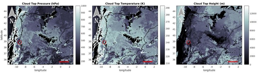
Figure 2. Cloud top temperature, pressure and height products representing the region of interest of
the spaceborne Spinning Enhanced Visible and Infrared Imager (SEVIRI) images used for this study.top pressure (CTP) and cloud top height (CTH) variables. Cloud top properties data are produced
by the Satellite Application Facility on Climate Monitoring (CM SAF) [26]. The CM SAF cloud
property dataset level-2 products (CLAAS version 2) are produced continuously at a 15 minute
sampling rate with a large pixel size resolution of about 15 km. The region of interest used for this
study is visualized in Figure 2. The final step was carried out, selecting the cloud top data pixel that
Remote Sens. 2019, 11, 966 5 of 14
contains in its interior the GNSS station.
Figure 2. Cloud
Figure 2. Cloud top
top temperature,
temperature, pressure
pressure and
and height
height products
products representing
representing the
the region
region of
of interest
interest of
of
the spaceborne Spinning Enhanced Visible and Infrared Imager (SEVIRI) images used for this
the spaceborne Spinning Enhanced Visible and Infrared Imager (SEVIRI) images used for this study. study.
The Lisbon area is marked with a red circle and the data corresponds to a heavy rain event that occurred
on 26 October 2015 at 01:00 with a precipitation rate of 20 mm/h.
2.4. GNSS Data Processing
The GNSS data processing was performed using the software package GAMIT (GNSS at MIT)
and GLOBK (Global Kalman filter) [27]. The first one processes double-differenced phase data to
estimate three-dimensional station coordinates, satellite orbits, Earth orientation parameters (EOP) as
well as the atmospheric measurements in a loose a priori solution. The second uses a Kalman filter,
combining the solution obtained from GAMIT with global geodetic solution experiments to accurately
estimate a final parameter solution. Five years of RINEX data from IGP0 station were processed in
daily double-difference sessions. Only GPS data were used in this study since the GAMIT/GLOBK
version (v10.6) used in the processing did not include the multi-GNSS capability yet. Tight constraints
to the ITRF14 (International Terrestrial Reference System 2014) were carried out. The ITRF14 used
global station coordinates and EOP provided from GNSS and other space geodetic techniques data
time series to update solutions from past years (i.e., 2008). A set of about 40 International GNSS Service
(IGS) stations spread across the globe were grouped, in order to assure precise coordinate estimate
and lower correlation for the atmospheric parameters. IGS precise final orbits were also used. The
data processing was executed in two distinct steps to attain the best possible tropospheric results.
The details of this methodology and its full parameterization can be found in Benevides et al. [28].
The zenith wet delay (ZWD) was the atmospheric parameter estimated for each station in the GNSS
processing and was obtained at a time sampling of 15 min. The ZWD was related to the tropospheric
water vapor, being converted to PWV using an empirical relationship calibrated to the regional climate
of the study area [29,30].
2.5. Data Handling and Integration
In order to create a consistent input configuration for the neural network processing, data derived
from different sources (GNSS station, meteorological station and SEVIRI) had to be harmonized. Hence,
the 15-min GNSS data sampling was averaged at a 1-hour rate to make it comparable with the hourly
measurements available for the precipitation, pressure, temperature and relative humidity values
provided by the meteorological station. The same procedure was executed for the cloud top variables
obtained from SEVIRI, being each 15-min measurement averaged in each hour, therefore minimizing a
larger portion of data with no registers. In this way, all the datasets were standardized and could be
introduced together into the neural network.
3. Results and Discussion
3.1. Neural Network Configuration
The primary variable used as the neural network input is the hourly precipitation. The group of
external input variables is formed by the PWV obtained from the GNSS station, pressure, temperatureRemote Sens. 2019, 11, 966 6 of 14
Remote Sens. 2019,
and relative 11, x FOR measured
humidity PEER REVIEW
by
the meteorological station and the CTT, CTP and CTH obtained 6 of 15
from SEVIRI cloud products. A total of 41427 time steps are originated from the 5 years of continuous
data. Table 1 summarizes the characteristics of the variables used in the neural network processing.
Table 1. Information regarding the neural network data variables used for this experiment.
Table 1. Information
Variable Name regarding the neural
Source network data Acronym
variables usedUnits
for this experiment.
Function
Hourly
Variable precipitation
Name Meteorological
Source station
AcronymRain mm/h
Units Input/Output
Function
Precipitable water vapor GNSS station PWV mm Input
Hourly precipitation Meteorological station Rain mm/h Input/Output
Pressure
Precipitable water vapor Meteorological
GNSS station station PWV P mm hPa Input
Input
Temperature
Pressure Meteorological
Meteorological station station P T hPa°C Input
Input
Temperature Meteorological station T ◦C Input
Relative Humidity Meteorological station RH % Input
RelativeTop
Cloud Humidity
TemperatureMeteorological
Remote station
sensing RH CTT %K Input
Input
Cloud Top Temperature Remote sensing CTT K Input
Cloud Top Pressure Remote sensing CTP hPa Input
Cloud Top Pressure Remote sensing CTP hPa Input
Cloud Top
Cloud Top HeightHeight Remote
Remote sensing sensing CTH CTH mm Input
Input
The NARX network used for this work is initially configured with a set of default parameters.
The NARX network used for this work is initially configured with a set of default parameters.
The network structure can be viewed in Figure 3. One hidden layer is selected for the input data
The network structure can be viewed in Figure 3. One hidden layer is selected for the input data
with 10 neurons (N) and one output layer is selected for the targets with a single neuron (M). The
with 10 neurons (N) and one output layer is selected for the targets with a single neuron (M). The
number of feedback (m) and input delays (n) are set to be the number of hours associated with the
number of feedback (m) and input delays (n) are set to be the number of hours associated with the
weather nowcasting limit, which is 6 hours [20]. The network function used for the training step is
weather nowcasting limit, which is 6 hours [20]. The network function used for the training step is the
the Levenberg–Marquardt algorithm, which is fast and does not require too much memory. The
Levenberg–Marquardt algorithm, which is fast and does not require too much memory. The network’s
network’s weight (w) and bias (b) structure is given by the architecture initially defined, relating the
weight (w) and bias (b) structure is given by the architecture initially defined, relating the number of
number of layers, neurons and inputs. The number of input weights is given by the number of
layers, neurons and inputs. The number of input weights is given by the number of neurons in the
neurons in the hidden layer (10) times the number of variables (8) and the number of input delays (6)
hidden layer (10) times the number of variables (8) and the number of input delays (6) resulting in a
resulting in a matrix with 480 elements. Additional parameters are the individual weight of each
matrix with 480 elements. Additional parameters are the individual weight of each neuron and the
neuron and the respective bias for the input and output layers, resulting in 21 additional weight
respective bias for the input and output layers, resulting in 21 additional weight elements (10 + 10 + 1).
elements (10 + 10 + 1). The input and output variables are scaled before training between −1 and 1, so
The input and output variables are scaled before training between −1 and 1, so that the weights are
that the weights are comparable and not unit dependent.
comparable and not unit dependent.
Figure 3. Structure of the nonlinear autoregressive exogenous neural network model (NARX) neural
network3.model
Figure usedofinthe
Structure thisnonlinear
work, where y(t+1) is theexogenous
autoregressive predicted variable, y(t) the model
neural network (NARX) x(t)
input variable, the
neural
exogenous
network inputused
model in thisnwork,
variables, the input
where y(t+1)misthe
delays, feedback
the delays,
predicted N and
variable, y(t)Mthe
theinput
number of layer’s
variable, x(t)
neurons
the and w and
exogenous b the
input respective
variables, weights
n the input and biases.
delays, m the feedback delays, N and M the number of
layer’s neurons and w and b the respective weights and biases.
The data division is setup in order to process the neural network in two steps. The goal is to
provide independent output precipitation values. In the first step we use a subset of 4 years of data
(5 years in total), setting the larger portion to the training set, 66%, the shorter portion to the validation
set, 10%, and 24% of the portion to the test. This way we assure that about 1 year of data is used
for results assessment. The sample selection for the data division is done randomly. In the second
processing step the trained network from the first step is used to forecast the rain using 1 year of data
not used in the training. Since the training is performed with a different data subset (4 years), the
output predicted precipitation values for one year are obtained in an independent manner. Table 2
summarizes the most important parameters of the neural network. The hourly precipitation continuous
data is characterized by its rapid temporal variability, including most cases of no rain to moderated rainRemote Sens. 2019, 11, 966 7 of 14
episodes and the more complex intense rainfall patterns, which are statistically not frequent. For this
reason, we have chosen to sum the rain values forward in time, but not surpassing the nowcasting
window threshold of 6 hours. This sum time window has been set initially and just for the precipitation
values, as 1 hour forward. A set of 100 runs is defined for each experiment, since the initial weights are
randomly generated in the neural network training phase, therefore affecting the fitting output results.
Consequently, the results are assessed in each experiment considering the mean or maximum values
obtained from the total number of runs.
Table 2. Information regarding the neural network default or initial parameters used for this work.
Variable Name Values
# Hidden layers 1
# Neurons 10
# Delays 6
Training function Levenberg-Marquardt
Data weighting Random
Performance evaluation Mean square error
Data division Step 1: (66%/10%/24%)—4 years
(training/validation/testing) Step 2: (0%/0%/100%)—1 year
# Total input variables 8
# Output variables 1
# Number of samples 41427
In order to better assess the potentiality of the method to forecast heavy precipitation, a classification
of the precipitation intensity is implemented. Thus, three classes are defined for the target and output
hourly precipitation, which are a class for non-raining values, an intermediated class regarding
moderated rain with values higher than 0 and lower than 5 mm/h and a final class corresponding to
more intense rain containing all values with precipitation reaching at least 5 mm/h. This threshold is
chosen considering the rain intensities observed in the region of study, where it is found that these
events at a rate of one hour represent about 0.5% of the total of rain occurrences during the study
period. Thereby, it can be stated that the intense rain in this region is considered as a rare event. The
precipitation classes and the number of trends can be observed in Table 3. This classification is applied
to the target rain values, considered as the measured or reference values and also applied to the output
data resulting from the neural network output. The classification for the output data considers a
0.5 mm/h tolerance in the moderated and intense rain classes. With this simple class clustering we can
test more clearly the capability of this method to identify correctly the heavy rain events.
Table 3. Details of the classification of precipitation data and the corresponding number of observations
concerning the neural network data division.
Number of Samples (hour)
Precipitation Class Rain Classification (mm/h)
4 Years 1 Year Total
No rain 0 31284 7527 38811
Moderated rain >0= 5 159 22 181
3.2. Network Sensitivity to Parameters
The first experiment was performed varying some of the initial parameters described in Table 2,
such as the number of default feedback and input delays, the number of hidden neurons and the
training function. The goal was to verify the possibility to improve the results obtained with the
default parameters. Nevertheless, some configurations were maintained, such as the number of input
variables and data division. The 4 years used in the data division of step 1 are 2011 to 2014, and for step
2 the remaining year 2015 was used for the assessment of results. The mean value was computed overRemote Sens. 2019, 11, 966 8 of 14
100 runs, for all the experiments. A statistical summary of the results is presented in Table 4, focusing
on the good classification and false positive percentages of the intense rain class. The percentage of
correctly classified intense rain was evaluated, relating the number of well-classified intense rain events
by the neural network processing with the real or observed rain values (in Table 3). The false positive
percentage was calculated, evaluating the total number of intense rain events wrongly classified by
the neural network experiment as intense rain. The statistical assessments also included the network
prediction error (Net.RMS), which is a mean squared normalized error calculated between the output
network values and the observed precipitation values, and the correlation coefficient for the step 2
dataset. The reference result values were obtained when using the network defaults parameters, leading
to a good classification percentage of 59.1%, with a 29.6% percentage of false positives, a network
RMS of 0.467 and a network correlation coefficient of about 0.824. The major differences between the
experiments summarized in Table 4 were obtained for the false positive percentages of the intense rain.
Table 4. Statistical assessment of the neural network experiments, comparing the initial and optimized
network parameters. Results correspond to the mean value score for 100 runs. Good classification and
false positives are presented in % of intense rain class, and network RMS is in mm/h.
Neural Network with 7 Variables Intense Rain Class Test Dataset
(GNSS+Meteo+Sat.)
Good False Correlation
Net.RMS
Classification Positives Coefficient
10 N, 6 ID 6 FD, Levenberg-Marquardt 59.1% 29.6% 0.467 0.824
10 N, 8 ID 8 FD,
59.1% 28.7% 0.470 0.821
Levenberg-Marquardt
2 N, 6 ID 6 FD, Levenberg-Marquardt 59.1% 26.4% 0.472 0.818
10 N, 6 ID 6 FD, Bayesian
59.1% 26.0% 0.489 0.803
regularization
The first tested parameter was the number of default feedback (FD) and input delay (ID) values.
These parameters varied equally between 1 to 10 delays. Similar intense classification results were
obtained with 1 to 4 delays, showing, however, larger false positive rate, higher network error and
smaller correlation. When testing with a number of 8 delays, the results were very similar to the
default ones (6 delays), showing similar good classification, error and correlation, while presenting a
small improvement on the false positive rate (28.7%). Increasing the number of delays to 10 resulted
in the same levels of error and correlation but it significantly increased the false positives rate. The
configuration of unbalanced delays was also tested with combinations of input delays and feedback
delays varying from 1 to 6. However, none of these configurations have provided better results for the
intense rain classification.
The following tested parameter was the neural network number of neurons. Experiments were
performed varying the neurons in the hidden layer from 1 to 25. Overall, the number of good
classifications remained unchanged, but the number of false positives decreased with fewer neurons in
the network. When using 1 neuron, the number of false positives was the lowest (22.2%), but with a
significant diminishment in the good classification of intense rain, higher network RMS and lower
correlation. However, when using 2 neurons the network reached 59.1% for good classification and
26.4% for false positive percentage, outperforming the intense rain classification for the default values.
Increasing the neurons by more than 2 did not improve the percentage of good classification, and
moreover it increased the false positive percentage. Additional tests extending the network complexity
with extra hidden layers were performed (see Figure 3). However, it was verified that as the number of
hidden layers increased, the percentage of good classification and correlation decreased, and the false
positive rate increased as well as the network error.
The final parameter testing was performed with the network training function. The neural
network initial parameters were restored again (10 neurons with 6 delays). We have chosen the training
functions that are most commonly used in this technique [31]. The statistical assessment using theRemote Sens. 2019, 11, 966 9 of 14
Quasi-Newton and Conjugate gradient training functions (not shown) revealed very poor results
when compared to the default Levenberg-Marquardt function. However, the Bayesian regularization
function achieved the same good classification percentage and managed to drop the false positive
percentage by more than 3% (26%) without a significant increase in the network error and a slight
decrease in the global correlation coefficient. The parameter variation experiments over the neural
network initial values and its statistical analysis of the intense rain classification revealed that some
parameters can be modified from the default values in order to improve the results. In the following
sections, the best individual parameters identified in these experiments—the 2 neurons with one
hidden layer, 8 delays and Bayesian regularization training function—are combined for additional
neural network proprieties testing.
3.3. Network Sensitivity to Input Variables
A set of tests was performed varying the number of input variables to better understand the
sensitivity of the neural network in terms of intense rain classification. In particular, given the
indicators of previous studies, emphasis was placed on the GNSS PWV. The network configuration
from Table 2 was used together with the implementation of the optimized network parameters
determined from the previous section (Table 4). The test results are presented in Table 5. The input
configuration with 7 variables and optimized parameters achieved an improvement of about 3% in
the false positive percentage, maintaining the same percentage of good classification compared with
the initial configuration result. When combining the GNSS and meteorological station variables, the
percentage of good classification slightly increased, and the false positive percentage also increased
to the maximum value of the experiment (27%). Processing the neural network with the PWV as
the only input resulted in a marginal higher good classification percentage (59.3%) and the lowest
percentage of false positives (22.6%). The last experiment was performed with a slight variation of
the NARX model configuration, which was running the network in NAR configuration mode, i.e.,
using only the y(t) precipitation as input (see Figure 3). The NAR results show the smallest percentage
of good classification (58.2%) with a similar false positives percentage to that obtained for the PWV
input configuration.
Table 5. Statistical assessment of the neural network input experiments with 4 different input configurations,
using optimized parameters. Results correspond to the mean value score for 100 runs. Good classification
and false positives are presented in % of intense rain class and Network RMS is in mm/h.
Neural Network with 7 Intense Rain Class Test Dataset
Variables # var.
Good False Correlation
(GNSS+Meteo+Satellite) Net.RMS
Classification Positives Coefficient
GNSS + Meteo. + Satellite
7 59.1% 26.5% 0.475 0.819
(PWV,P,T,RH,CTT,CTP,CTH)
GNSS + Meteo. (PWV,P,T,RH) 4 58.9% 27.1% 0.471 0.821
GNSS (PWV) 1 59.3% 22.6% 0.471 0.817
Precipitation (NAR model) 1 58.2% 22.7% 0.474 0.815
The network error and correlation coefficient of the optimized experiments are marginally larger
than that observed for the initial network configuration. This is probably related to the decrease in the
number of neurons, as it was verified in the previous section. However, between these experiments,
the error and correlation variations are very small, the best score being obtained for the 4 exogenous
input variables. Summarizing the results of this experiment, it was observed that introducing more
variables into the neural network processing does not produce the better results. The best classification
scores of the intense rain events are obtained for the input exogenous configuration with GNSS PWV.
When introducing more external variables from different sources (meteorological station and satellite
SEVIRI cloud top data) the network error generally increases.Remote Sens. 2019, 11, 966 10 of 14
3.4. Network Sensitivity to Data Division
In this section, the neural network sensitivity is evaluated, varying the data division in time. The
data division configuration defined in the neural network configuration section is modified, setting up
experiments using each year of the full 5-year dataset as a test year (step 2 of Table 2). The remaining
data in each experiment are evenly distributed by the training, validation and test of step 1, keeping
the percentages of data division previously defined in Table 2. These experiments consider the neural
network optimized configuration. A helpful indicator for the nowcasting of heavy rain is to consider
the maximum value from the 100 runs processed in each experiment, which is derived from the highest
percentage of good classification and lowest percentage of false positives of the intense rain class. The
input configuration used for this experiment is the exogenous input PWV variable.
The statistical assessment shown in Table 6 shows quite stable performances in the intense rain
classification. These results seem also to confirm that we are not faced with the overfitting problem.
The 2013 dataset has the lowest percentage of false positives (21%) with a high percentage of good
classification (66%), also showing intermediate intense rain events (37). The year with the poorer
intense rain classification is 2011, with the smallest good classification (63%) and the highest percentage
of false positives (36%), although being characterized by the highest number of intense rain events
(57). The 2015 dataset has similar good classification score but with a much lower false positive rate
(22%), being also the year with the smallest number of intense rain events (22), an indicator of a
dryer year. The year 2012 shows the highest percentage of good classification, reaching 72% with a
relatively low false positive percentage of 23%, showing a relatively small network error (0.59) and
the highest correlation coefficient (0.88). The higher variability in the neural network performance
in this test is a direct consequence of a different number of intense rain data registered in each year.
However, the variability in the network error and correlation also suggests that the data available for
the training and validation steps may not be sufficient to provide a robust model for the intense rain
prediction in all weather conditions. On the other hand, the smaller network error obtained in the 2015
dataset is a consequence of the testing period being all continuous, that is, not being interrupted by
a segmented year from the middle of the dataset. Nevertheless, the result of this experiment shows
that the methodology presented here has potential to be used as a tool for assisting in the intense rain
forecast nowcasting. Comparing with results from previous studies introduced in Section 1 [11–13],
and even though these studies consider all the types of rain, a significant improvement in the false
positive rate with registers of 36% down to 21% is observed, just considering the heavy rain events.
The following section explores in more detail the properties of the neural network for the dataset in
continuous mode, using the most recent year (2015) for results assessment.
Table 6. Statistical assessment of the neural network experiment with variations in the data division.
Optimized parameters and PWV exogenous input variable configuration is considered. Results
correspond to the maximum value score for 100 runs. Good classification and false positives are
presented in % of intense rain class, and Network RMS is in mm/h.
Neural Network with 7 Intense Rain Class Test Dataset
Variables #Intense Rain
Good False Correlation
(GNSS+Meteo+Satellite) Net.RMS
Classification Positives Coefficient
2015 test dataset 22 63.6% 22.2% 0.464 0.826
2011 test dataset 57 63.3% 35.6% 0.875 0.828
2012 test dataset 32 71.9% 23.3% 0.589 0.875
2013 test dataset 37 66.0% 20.5% 0.807 0.820
2014 test dataset 41 64.3% 30.8% 0.726 0.831
3.5. Best Case with Optimized Parameters
The best result for the most recent year of the data series is analyzed here (optimized parameters 2
neurons with one hidden layer, 8 delays and Bayesian regularization training function, GNSS PWV, oneneural network for the dataset in continuous mode, using the most recent year (2015) for results
assessment.
3.5. Best Case with Optimized Parameters
Remote Sens. 2019, 11, 966 11 of 14
The best result for the most recent year of the data series is analyzed here (optimized
parameters 2 neurons with one hidden layer, 8 delays and Bayesian regularization training function,
GNSS PWV,
exogenous one exogenous
variable variable
configuration, best configuration,
intense rain score bestinintense rainfor
100 runs score in 100test
the 2015 runs for theFigure
dataset). 2015 4
test dataset). Figure 4 shows hourly the rainfall in situ measurements and forecasts
shows hourly the rainfall in situ measurements and forecasts provided by the neural network output. provided by the
neural network output. These values are concentrated in the region of low-intensity rainfalls, smaller
These values are concentrated in the region of low-intensity rainfalls, smaller than 5 mm/h, and have a
than 5 mm/h, and have a correlation coefficient of 0.83. The differences between the predicted and
correlation coefficient of 0.83. The differences between the predicted and observed values increase
observed values increase gradually, not predicting some of the higher observed rain events. The
gradually, not predicting some of the higher observed rain events. The comparison of predicted and
comparison of predicted and observed values through the year 2015 shows a good coverage of the
observed values through the year 2015 shows a good coverage of the rain events, where the predicted
rain events, where the predicted values seem to be more underestimated than overestimated.
values seemrainfall
Different to be more underestimated
patterns than overestimated.
can be observed throughout theDifferent
year, withrainfall patterns
a drier period can
frombeJuly
observed
to
throughout the year, with a drier period from July to September, and some rainier
September, and some rainier months like January, April and October. Most of the output values aremonths like January,
April and October.
concentrated Most
in the of the
region output
around values
zero, with aare concentrated
more noticeable in the concentration
noisy region aroundofzero, with
rainfall a more
values
noticeable noisy concentration
in the month of October. of rainfall values in the month of October.
(a) (b)
Figure
Figure 4. 4.Linear
Linearfitting
fittingbetween
between the
the predicted
predicted rain
rainvalues
valuesfrom
fromthe
theneural
neuralnetwork
network and thethe
and observed
observed
rain values, in units of mm/h, for the year 2015 (a). The same
rain values, in units of mm/h, for the year 2015 (a). The same comparison comparison is illustrated for
for all values
all values of
the year 2015 organized by time (b). Results correspond to the best score for 100 runs withwith
of the year 2015 organized by time (b). Results correspond to the best score for 100 runs the the
initial
initial network
network parameters
parameters set in2.Table 2.
set in Table
As a further assessment of the proposed methodology, a confusion matrix is used to assess the
classification results of the whole rainfall datasets. Figure 5 summarizes the results of the confusion
matrix. In this form we can evaluate the precipitation considering the classification of the output
values (row-wise) versus the classification of the reference or measured values (column wise), also
known as the ground truth. The matrix shows all the 2015 dataset precipitation values distributed
by classes, where the diagonal position represents the number of correctly classified precipitation
events. The marginal bottom row shows the global percentage of correctly classified trends obtained
for the output values (green percentage) with respect to the measured values, and also the percentage
of omission errors for each class (red percentage), determined from the non-diagonal overclassified
events. As for the marginal right end column, it identifies for the classification output, the percentage
of correctly classified events in each class (green percentage) and its commission error or false positive
rate (red percentage). The highest ground truth classification is obtained for the no rain class, with
almost 100% of well-classified events, followed by the intense rain with about 64% and the moderated
rain with 35%. As for the output classification, the no rain also has the highest score, with 98%. The
moderated rain also has a better classification score with 77% of the values well-classified, while the
class of interest, the intense rain, manages to achieve about 78% well-classified output events with
a false positive rate of about 22%. The overall classification accuracy is very good, achieving 97.5%.
In addition to the previously demonstrated neural network capacity to forecast heavy rain events
with high correctness and low false positive rate, the confusion matrix shows that this method has
also a remarkable hit success for the no rain events, being near 100%. This property can be useful
in meteorological applications where the knowledge of the rain/no rain factor is important, such as
precision farming.accuracy is very good, achieving 97.5%. In addition to the previously demonstrated neural network
capacity to forecast heavy rain events with high correctness and low false positive rate, the confusion
matrix shows that this method has also a remarkable hit success for the no rain events, being near
100%. This property can be useful in meteorological applications where the knowledge of the
rain/no
Remote Sens.rain
2019,factor
11, 966 is important, such as precision farming. 12 of 14
Figure 5. Confusion matrix relating the precipitation forecast provided by the neural network output
Figure 5. Confusion matrix relating the precipitation forecast provided by the neural network output
and the observed or measured rainfall input (ground truth), classified after the neural network result
and the observed or measured rainfall input (ground truth), classified after the neural network result
using Table 3. Results correspond to the best score for 100 runs with the optimized network parameters
using Table 3. Results correspond to the best score for 100 runs with the optimized network
(2 neurons, 1 hidden layer, 8 feedback and input delays and Bayesian training), Global Navigation
parameters (2 neurons, 1 hidden layer, 8 feedback and input delays and Bayesian training), Global
Satellite System (GNSS) precipitable water vapor (PWV) one input variable configuration and test
Navigation Satellite System (GNSS) precipitable water vapor (PWV) one input variable
dataset 2015.
configuration and test dataset 2015.
4. Conclusions
4. Conclusions
A large dataset of continuous GNSS measurements of PWV, meteorological measurements and
A large
spaceborne dataset
SEVIRI of continuous
images has been GNSS
analyzedmeasurements
by means ofofneural
PWV,network
meteorological measurements
NARX method. and
The goal
spaceborne SEVIRI images has been analyzed by means of neural network NARX method.
was to find a relationship between atmospheric and cloud properties and in situ rainfall measurements The goal
towas to find
be used for thea nowcasting
relationshipofbetween atmospheric
intense rain events. A and cloud
total set of 7properties and in from
variables obtained situ GNSS
rainfall
measurements
and meteorological to be used for the nowcasting
measurements of intense
were gathered, rain events.toAfive
corresponding totalyears
set ofof7 continuous
variables obtained
data,
and introduced into the neural network in order to estimate hourly precipitation. Classification ofof
from GNSS and meteorological measurements were gathered, corresponding to five years
continuous
output resultsdata, and introduced
is performed in threeinto theclasses
rain neuraltonetwork in order
assess the to estimate
method’s intensehourly precipitation.
rain forecast skill.
Classification of output results is performed in three rain classes to assess the method’s
Several experiments have been carried out with different initial conditions for the neural network intense rain
parameters. For each parameter’s configuration, a set of 100 runs was used for the statistical assessment
of forecast results. Tests evaluating the neural network sensitivity to different parameters found that
the best results for the classification of intense rain events were obtained for network configuration of
2 neurons, 1 hidden layer, 8 feedback and input delays and Bayesian regularization training. Tests
performed varying the number of the neural network exogenous variables revealed that using all
input variables, including data from meteorological station and cloud top information from SEVIRI
images, resulted in a reduced capability of the neural network to correctly classify the intense rain
events. Better classification results were obtained when using only the GNSS PWV variable (64% good
classification, 22% false positives). The reason for this could be related to the different acquisition
proprieties regarding the ground-based GNSS and meteorological stations, and the spaceborne SEVIRI
imaging. GNSS uses a mean of all satellite observations to estimate the total column of PWV, which is
basically referring to the lower tropospheric layer, while the metrological station measures quantities
at the surface level. On the other hand, SEVIRI is measuring the quantities at the top of the clouds
(see Figure 2 for the statistical distribution of cloud heights), not observing most of the time, the
same portion of troposphere as the ground sensors, particularly in the presence of clouds, which are
the rain trigger. Therefore, the physical quantities of the GNSS, metrological station and SEVIRI are
poorly correlated, and the lower part of the troposphere sensed from the GNSS stations could be more
important to study the precipitation behavior.
Comparisons with previous studies showed that the proposed methodology has a better
performance, achieving a significant reduction in the severe rain false positives forecast. The experiment
evaluating the network sensitivity to different years of independent measurements revealed very
distinct results, probably due to the number of intense rain events registered in each year. Longer timeRemote Sens. 2019, 11, 966 13 of 14
series of many years would be desirable, as well as other GNSS location, in order to better model the
complex behavior of the precipitation phenomena and its different regimes observed even in consecutive
years. These results support the idea of the usefulness of a data-driven analysis of atmospheric and
rainfall measurements based on a neural network methodology in applied meteorology as an auxiliary
tool for the short-term forecast of heavy rainfall events. As a co-product of this study, it has been
observed that the presented methodology has a near 100% hit success for the no rain event classification,
with almost no false positives. This result can be of interest in applications tightly related to applied
meteorology, such as precision farming, where the information of a lack of rainfalls has an important
economic value in agricultural practices.
Author Contributions: Conceptualization, J.C. and P.B.; methodology, J.C. and P.B.; validation, P.B.; formal
analysis, P.B.; investigation, P.B., J.C. and G.N.; writing—original draft preparation, P.B.; writing—review and
editing, P.B., J.C. and G.N.; visualization, P.B.; supervision, J.C. and G.N.
Funding: This research was funded by Fundação para a Ciência e Tecnologia (FCT), project UID/GEO/50019/
2019—Instituto Dom Luiz.
Acknowledgments: The authors would like to thank the DGT for providing freely the GNSS data and the CM
SAF for providing freely the SEVIRI cloud property dataset level-2 products.
Conflicts of Interest: The authors declare no conflict of interest.
References
1. Yan, X.; Ducrocq, V.; Poli, P.; Hakam, M.; Jaubert, G.; Walpersdorf, A. Impact of GPS zenith delay assimilation
on convective-scale prediction of Mediterranean heavy rainfall. J. Geophys. Res. Atmos. 2009, 114. [CrossRef]
2. Mateus, P.; Miranda, P.M.A.; Nico, G.; Catalão, J.; Pinto, P.; Tomé, R. Assimilating InSAR maps of water
vapor to improve heavy rainfall forecasts: A case study with two successive storms. J. Geophys. Res. Atmos.
2018, 123, 3341–3355. [CrossRef]
3. Brenot, H.; Neméghaire, J.; Delobbe, L.; Clerbaux, N.; De Meutter, P.; Deckmyn, A.; Delcloo, A.; Frappez, L.;
Van Roozendael, M. Preliminary signs of the initiation of deep convection by GNSS. Atmos. Chem. Phys.
2013, 13, 5425–5449. [CrossRef]
4. Mateus, P.; Nico, G.; Catalao, J. Uncertainty Assessment of the Estimated Atmospheric Delay Obtained by a
Numerical Weather Model (NMW). IEEE Trans. Geosci. Remote Sens. 2015, 53, 6710–6717. [CrossRef]
5. Guerova, G.; Jones, J.; Douša, J.; Dick, G.; Haan, S.D.; Pottiaux, E.; Bock, O.; Pacione, R.; Elgered, G.; Vedel, H.;
et al. Review of the state of the art and future prospects of the ground-based GNSS meteorology in Europe.
Atmos. Meas. Tech. 2016, 9, 5385–5406. [CrossRef]
6. Suparta, W.; Ali, M. Nowcasting the lightning activity in Peninsular Malaysia using the GPS PWV during
the 2009 intermonsoons. Ann. Geophys. 2014, 57, A0217. [CrossRef]
7. Barindelli, S.; Realini, E.; Venuti, G.; Fermi, A.; Gatti, A. Detection of water vapor time variations associated
with heavy rain in northern Italy by geodetic and low-cost GNSS receivers. Earth Planets Space 2018, 70, 28.
[CrossRef]
8. De Haan, S. Assimilation of GNSS ZTD and radar radial velocity for the benefit of very-short-range regional
weather forecasts. Q. J. R. Meteorol. Soc. 2013, 139, 2097–2107. [CrossRef]
9. Benevides, P.; Nico, G.; Catalao, J.; Miranda, P.M.A. Analysis of Galileo and GPS Integration for GNSS
Tomography. IEEE Trans. Geosci. Remote Sens. 2017, 55, 1936–1943. [CrossRef]
10. Dousa, J.; Vaclavovic, P. Real-time zenith tropospheric delays in support of numerical weather prediction
applications. Adv. Space Res. 2014, 53, 1347–1358. [CrossRef]
11. Benevides, P.; Catalao, J.; Miranda, P.M.A. On the inclusion of GPS precipitable water vapour in the
nowcasting of rainfall. Nat. Hazards Earth Syst. Sci. 2015, 15, 2605–2616. [CrossRef]
12. Yao, Y.; Shan, L.; Zhao, Q. Establishing a method of short-term rainfall forecasting based on GNSS-derived
PWV and its application. Sci. Rep. 2017, 7, 12465. [CrossRef]
13. Manandhar, S.; Lee, Y.H.; Meng, Y.S.; Yuan, F.; Ong, J.T. GPS-Derived PWV for Rainfall Nowcasting in
Tropical Region. IEEE Trans. Geosci. Remote Sens. 2018, 56, 4835–4844. [CrossRef]
14. French, M.N.; Krajewski, W.F.; Cuykendall, R.R. Rainfall forecasting in space and time using a neural network.
J. Hydrol. 1992, 137, 1–31. [CrossRef]You can also read