Probabilistic Mangrove Species Mapping with Multiple-Source Remote-Sensing Datasets Using Label Distribution Learning in Xuan Thuy National Park ...
←
→
Page content transcription
If your browser does not render page correctly, please read the page content below
remote sensing
Article
Probabilistic Mangrove Species Mapping with
Multiple-Source Remote-Sensing Datasets Using
Label Distribution Learning in Xuan Thuy National
Park, Vietnam
Junshi Xia 1, *,† , Naoto Yokoya 1,2           and Tien Dat Pham 1
 1 Geoinformatics Unit, RIKEN Center for Advanced Intelligence Project (AIP), Tokyo 103-0027, Japan;
   naoto.yokoya@riken.jp (N.Y); tiendat.pham@riken.jp (T.D.P)
 2 Department of Complexity of Science and Engineering, The University of Tokyo, Chiba-ken 277-8561, Japan

 * Correspondence: junshi.xia@riken.jp; Tel.: +81-3-6225-2482
 † Current address: Nihonbashi 1-Chome Mitsui Building, 15th Floor, 1-4-1 Nihonbashi, Chuo-ku,
   Tokyo 103-0027, Japan.

 Received: 23 October 2020; Accepted: 20 November 2020; Published: 22 November 2020

 Abstract: Mangrove forests play an important role in maintaining water quality, mitigating climate
 change impacts, and providing a wide range of ecosystem services. Effective identification
 of mangrove species using remote-sensing images remains a challenge. The combinations of
 multi-source remote-sensing datasets (with different spectral/spatial resolution) are beneficial to
 the improvement of mangrove tree species discrimination. In this paper, various combinations
 of remote-sensing datasets including Sentinel-1 dual-polarimetric synthetic aperture radar (SAR),
 Sentinel-2 multispectral, and Gaofen-3 full-polarimetric SAR data were used to classify the mangrove
 communities in Xuan Thuy National Park, Vietnam. The mixture of mangrove communities consisting
 of small and shrub mangrove patches is generally difficult to separate using low/medium spatial
 resolution. To alleviate this problem, we propose to use label distribution learning (LDL) to provide
 the probabilistic mapping of tree species, including Sonneratia caseolaris (SC), Kandelia obovata (KO),
 Aegiceras corniculatum (AC), Rhizophora stylosa (RS), and Avicennia marina (AM). The experimental
 results show that the best classification performance was achieved by an integration of Sentinel-2
 and Gaofen-3 datasets, demonstrating that full-polarimetric Gaofen-3 data is superior to the
 dual-polarimetric Sentinel-1 data for mapping mangrove tree species in the tropics.

 Keywords: mangrove species mapping; label distribution learning; Gaofen-3; Sentinel; Vietnam

1. Introduction
     Mangrove ecosystems can provide a range of essential ecological services, including (1) impact
reduction for natural disasters, (2) habitat provision for coastal wildlife, and (3) blue carbon
sequestration in the coastal zone [1–3]. However, due to human activities and environmental
degradation, mangrove forests have been significantly lost regionally and globally [4]. Thus,
mapping and monitoring mangrove are imperative to building a good understanding of the
current conditions, their dynamics, and further support the coastal blue carbon conservation and
management [5,6].
     Recently, many approaches have been proposed to map mangrove tree species using optical
and synthetic aperture radar (SAR) data with various spectral/spatial/temporal resolutions [7–12].
Medium resolutions datasets, including Sentinel and Landsat series [2], have been widely used to map the
changes of large areas of mangrove. With the advantages of providing more detailed spectral and texture

Remote Sens. 2020, 12, 3834; doi:10.3390/rs12223834                    www.mdpi.com/journal/remotesensing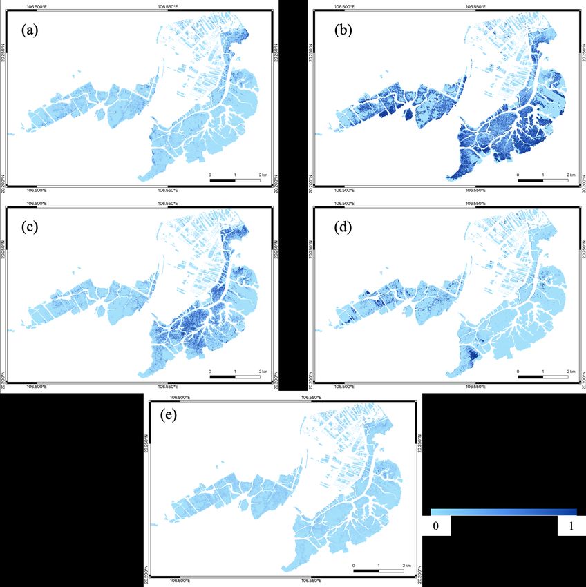
Remote Sens. 2020, 12, 3834                                                                           2 of 17

information, hyperspectral and high-resolution datasets are also intensively used for discriminating
mangrove species. Wan et al. [13] have investigated four mangrove species in Hong Kong using the
new hyperspectral Gaofen-5 dataset (330 spectral bands). Besides the conventional satellite sensors,
such as Worldview [14] and Pleiades [15], unmanned aerial vehicles (UAVs) [16] have been employed
for mangrove mapping, especially for individual mangrove analysis, in which the fuzzy-based and
objected-based approaches are often adopted [8,12]. Since SAR images can penetrate the canopy and
sensitive to the surface and vertical structure, thus, they are useful for mapping and monitoring mangrove
structure and biomass [17,18]. Hence, various SAR datasets, such as ALOS, Radarsat, Sentinel-1, are used
to investigate mangroves communities distribution [19–21]. Mougin et al. [22], Proisy [23] analyzed
different frequencies (C-/L-/P-band) and polarizations for the mangrove tree species mapping and
biomass estimation [18].
       The current literature shows that multi-source remotely sensed datasets (e.g., optical, SAR and LiDAR)
are able to provide complementary information [24,25], their combinations can improve the classification
performance of mangrove mapping and monitoring. For instance, Souza and Paradella [26] used
Radarsat SAR and Landsat optical datasets for coastal mangrove mapping in the Amazon region.
Different combinations, including hyperspectral and ENVISAT SAR [27,28], multi-tidal Landsat
and a Digital Elevation Model (DEM) [29], was used for mangrove tree species mapping [27,28].
Zhang et al. [1] adopted a rotation forest classifier for the mangrove tree mapping with the integration of
Worldview-3 and Radarsat-2 data.
       As a part of the China High-Resolution Earth Observation System (CHEOS), Gaofen-3 (GF,
“High Resolution”) is the first civilian C-band polarimetric SAR imaging satellite of CNSA (China
National Space Administration) [30]. The GF-3 satellite has 12 imaging modes, including spotlight,
stripmap, and scan, with four polarization capabilities and the highest resolution of 1 m. Previous
studies have already confirmed the effectiveness of using optical Gaofen-1 [31] and Gaofen-2 [32] for
the extraction of mangrove tree species. More recently, Zhu et al. [33] has integrated GF-2 Optical,
GF-3 SAR, and UAV to estimate biomass of mangroves. However, the mangrove classification
performance of using full-polarimetric GF-3 SAR has not yet been investigated.
       In most cases, pixel-wise and objective-based classifications are employed to medium/low-
and high-spatial-resolution images, respectively. However, the mixture of mangrove communities
and the low spatial resolution of the datasets bring the challenge to separate mangrove tree species.
In mixed-pixel studies, the sub-pixel or spectral unmixing techniques have been widely used [15,34].
However, they need the “pure” pixels (i.e., one label for one pixel) as the input. In most cases,
the “pure” pixels are very hard to find in real scenarios. In such case, it is better to use soft labels
(i.e., multiple labels in one pixel) instead of the one label of “pure” pixels. In this work, we propose
to use a new machine learning paradigm, namely label distribution learning (LDL) [35], which uses
the soft labels as the input. The label distribution covers multiple labels, representing the degree (i.e.,
probability) to which each label describes the pixel [35]. The objective of LDL is to predict multiple
real-valued description degrees (i.e., probabilities) of the labels. The LDL methods have widely used
in many machine learning applications, such as facial age estimation [36], head pose estimation [37],
emotion distribution recognition [38], etc.
       To date, there have been no attempts to map mangrove communities, including mixed several
small and shrub mangrove patches despite these mangrove species being crucial to coastal zones in
mitigating storm surges impacts and defending against rising sea levels [39]. Accordingly, the current
work attempts to fill this gap by investigating multi-source optical and SAR remote sensing datasets
and the label distribution learning (LDL) techniques [35] to map mangrove tree species in the mangrove
ecosystem of the National Park located in North Vietnam using the combination of GF-3 SAR and
optical datasets.
       The main contributions are listed as follows:

1.    exploiting GF-3 SAR to classify mangrove tree species for the first time.
2.    investigating the combination of GF-3 full-polarimetric SAR and Sentinel-2 optical datasets.
Remote Sens. 2020, 12, 3834                                                                              3 of 17

3.    proposing to use LDL for the probabilistic mangrove species mapping.

2. Materials and Methods

2.1. Study Area
     In this work, we selected the first Ramsar site in south-east Asia, namely Xuan Thuy National Park,
as the study area (shown in Figure 1). It is in the Northern coastal area of Nam Dinh province, Vietnam.
The study area is classified as the tropical monsoon area with two distinct dry (from November to next
April) and rainy seasons (from May to October) [40].
     The total area of this park is approximately 15,000 ha, of which about 7100 and 8000 ha are the core
and the buffer zones, respectively. The mangrove tree densities varied at different zones of Xuan Thuy
National Park, Nam Dinh Province. We observed the number of mangrove stands was higher in the
core zone than those in the buffer and transition zones, ranging from 315 to 8285 tree ha −1 . The number
of mangrove trees depends on the specific locations of the study area. In the buffer and transition
zones, the number of trees are relatively less than in the core zone of the National Park. We counted
all mangrove stands including small and shrub mangrove trees in 55 sampling plots at a size of
10 m × 10 m. We observed five dominant mangrove species, including Sonneratia caseolaris (SC),
Kandelia obovata (KO), Aegiceras corniculatum (AC), Rhizophora stylosa (RS), and Avicennia marina (AM),
during the fieldwork.

      Figure 1. (a) The study area, Xuan Thuy National Park, is located at the estuary of the Red River in
      Nam Dinh province, about 150 km south east of Hanoi. (b) The detailed mangrove map, which was
      obtained from the Vietnam Forest Inventory and Planning Institute (FIPI), has shown the locations of
      55 sample sites as training samples, and 71 additional sample sites as test samples.

2.2. Remote-Sensing Data
    Figure 2 shows the main steps of remote-sensing image processing and the mangrove species
mapping using the LDL. First, the preprocessing steps were applied to Sentinel-1, Sentinel-2 and GF-3
datasets. Furthermore, data transformation was applied to Sentinel-2 and GF-3 datasets to obtain
vegetation indices and decomposition features. The probabilities derived from 55 sample sites were
Remote Sens. 2020, 12, 3834 4 of 17
used to train the LDL. Then, the probabilities map of tree species in the study area were generated.
Finally, we used the descending probabilities from 71 sample sites to perform the accuracy assessment.
Figure 2. Flowchart of the proposed methods.
2.2.1. Remote-Sensing Pre-Processing
In this work, we selected Sentinel-1, Sentinel-2 and Gaofen-3 as the data source (Figure 3).
Sentinel-1 and Sentinel-2 datasets were downloaded from the Copernicus Open Access Hub (https:
//scihub.copernicus.eu) run by the European Space Agency (ESA), whereas the GF-3 dataset was
acquired from the China National Space Administration (CNSA).
For the Sentinel datasets, we chose the best quality images acquired in 2017 or in 2018
corresponding to the dates we did the field survey. In this case, we selected the Sentinel-2
acquired on 2 November 2018 and the Sentinel-1 dual-polarimetric SAR (VH and VV) obtained on
16 December 2017. For GF-3 datasets, we selected the full-polarimetric datasest using the acquisition
mode of Quad-pol stripmap (QPSI).
GF-3 full-polarimetric SAR is very limited in this area. Since the recent GF-3 image is acquired
on 27 December 2016, therefore, we selected this one in our studies. Since there is almost no change
between 2016 and 2018 in this area, the influences of different dates can be ignored. The main
parameters of Sentinel-1, Sentinel-2 and GF-3 are given in Table 1.
Table 1. The main parameters of the Remote-Sensing products used in this study.
Satellite Acquisition Date Mode Bands Spatial Resolution (m)
Sentinel-1 16 December 2017 Dual-Polarization VH, VV 10
Sentinel-2 2 November 2018 Multispectral Imager (MSI) 11 spectral bands 10/20
GaoFen-3 27 December 2016 Full-Polarization HH, HV, VH, VV 8
For the Sentinel-1 (S1) images, the following steps, including noise removal, calibration, speckle
filtering, and geometric correction were applied to the VV and VH polarimetric bands and then
converted to backscattering coefficients in decibel (db) unit. For the Sentinel-2 (S2) images, Sen2Cor
algorithm was used for the atmospheric correction [17]. For the GF-3 datasets, the calibration constantsRemote Sens. 2020, 12, 3834 5 of 17
were used to correct the backscattering coefficient information on different polarization channels. Then,
the multi-look was applied to de-speckle the image. The polarimetric coherency matrix was generated,
and the refined Lee filter was used to reduce the speckle noise.
Figure 3. (a) False composite color image of Sentinel-1 (R:VH, G:VV, B:VV) acquired on 16 December
2017, (b) True composite color image of Sentinel-2 (R: Band 4, G: Band 3, B: Band 2) acquired
on 2 November 2018. (c) False composite color image of GF-3 (R:HH, G:HV, B:VV) acquired on
27 December 2016. The land cover types surrounding the mangroves contain sea water, agriculture,
tidal mudflat, salt field, built-up areas etc [41].
2.2.2. Transformation of Sentinel-2 and GF-3
In addition to spectral bands of Sentinel-2, 7 vegetation indices (VIs) derived from S2 (see in
Table 2) were used in this study. It should be noted that all the spectral bands and vegetation indices
(i.e., S2+VIs in short) were used as the input of the LDL methods.
Table 2. Vegetation indices used in the study.
Vegetation Index Equation
B8− B4
Normalized Difference Vegetation Index (NDVI) [42] B8+ B4
Difference Vegetation Index (DVI) [43] B8 − B4
B5− B4
Normalized Difference Index using B4 and B5 (NDI45) [44] B5+ B4
B8
Ratio Vegetation Index (RVI) [45] B4
Soil Adjusted Vegetation Index (SAVI) [46] 1.5 B8+B8 − B4
2.4B4+0.5
B7− B4
Inverted Red-Edge Chlorophyll Index (IRECI) [47] B5/B6
B8− B3
Green Difference Vegetation Index (GNDVI) [48] B8+ B3
Note: B8 = NIR, B7= Vegetation red edge, B4 = Red.Remote Sens. 2020, 12, 3834 6 of 17
For GF-3, the Pauli and Krogager decompositions [49,50] were applied to the distribution of
mangrove species. Thus, in addition to four polarization channels (HH, HV, VH, VV), three Krogager
components, including diplane (KD), helix (KH), and sphere (KS), three Pauli parameters, including
odd-bounce scattering (P1), even-bounce scattering (P2), and volume scattering (P3), were included to
map the mangrove species distribution.
Finally, we resampled all the features derived from S1, S2, and GF-3 to a resolution of 10 m to
match the same size of sampling sites.
2.2.3. LDL Classification
Label Distribution Learning (LDL), which is proposed by Geng et al. [35], is a novel machine
learning paradigm, aim of which is to minimize the distance between the model output and the
ground-truth label distribution. In this work, we used the LDL packages from [35] (http://ldl.
herokuapp.com/download).
y
Let us denote the degree (i.e., probability) of label y to pixel x by dx . The label distribution of xi is
y1 y2 yc yj yj
given by Di = {dxi , dxi , . . . , dxi }, with the constraints of dx ∈ [0, 1] and ∑cj=1 dx = 1, where c is the
number of classes.
The LDL aims at predicting the probabilities of pixels or learn a conditional probability p(y|x)
from a training set {(x1 , D1 ), (x2 , D2 ), . . . , (xn , Dn )}. In general, the LDL approaches can be divided
into three categories: problem transformation, algorithm adaptation, and specialized algorithms [35].
Problem transformation methods directly convert the LDL problem to the existing single-label
learning (SLL) problem. In this case, problem transformation methods change the training examples
into weighted single-label examples.
More specifically, each training sample (xi , Di ) is transferred into c single-label samples (xi , y j )
yj
with the weights of dxi . The redefined training set, which includes c × n samples, is treated as the
single-label training set. In order to predict the class probability of test sample x, the selected learning
method should be able to produce the probability. In this case, two typical methods are the Bayes [51]
and the support vector machines (SVMs) classifiers [52]. The former assumes the data in Gaussian
distribution and uses the Bayes rule to produce the probabilities. The latter estimates the probabilities
by a pairwise coupling multi-class method. Problem transformations with the Bayes and the SVMs are
referred to as “PT-Bayes” and “PT-SVMs”.
Algorithm adaptation extends the existing methods to deal with label distributions.
In particular,the k-NN and the back-propagation neural network (BPNN) are adopted. We refer
them to “AP-kNN” and “AP-BPNN”, respectively. In this work, k is set to be 3.
In AP-kNN, the probability of new sample x is averaged by the probabilities of its k
nearest neighbors:
1 yj
p ( y j |x) = ∑ d xi
k i∈ N
(1)
(x)
k
where Nk (x) is the k nearest neighbors of x.
In AP-BPNN, the SoftMax activation function was used to generate the probability output.
Assume that the j−th output of AP-BPNN is v j , the output z j (z j ∈ [0, 1] and ∑ j z j = 1) is:
exp(v j )
zj = , ( j = 1, 2, . . . , c) (2)
∑ck=1 exp(vk )
The previous problem transformation and algorithm adaptation methods are an indirect strategy,
and the performance is very limited [35,53]. In this case, we need the specialized algorithms to directly
solve the LDL problem.Remote Sens. 2020, 12, 3834 7 of 17
Suppose p(y|x; θ) is a parametric model with a parameter vector θ. The two distributions can be
measured by Euclidean distance, Kullback–Leibler (KL) divergence etc. If we adopt the KL divergence,
the best parameter vector θ∗ can be determined in the following
yj
θ∗ = arg max ∑ ∑ dxi ln p(y|x; θ) (3)
θ i j
To directly tackle the optimization problem, Improved Iterative Scaling (IIS) [54] and
Broyden–Fletcher–Goldfarb–Shanno (BFGS) [55] are adopted. Here, we refer to them as “SA-IIS”
and “SA-BFGS”, respectively. Both the methods assume p(y|x; θ) to be the maximum entropy model.
SA-IIS uses a strategy similar to Improved Iterative Scaling (IIS) to maximize the likelihood of the
maximum entropy model. The SA-BFGS uses a quasi-Newton method BFGS as its optimization
algorithm. More detailed information about the SA-IIS and the SA-BFGS techniques can be found
at [35].
2.3. Field Data and Validation Analysis
Field experiments were carried out during the dry season (November and December 2018).
We conducted the measurements of 55 sampling sites with a square size of 100 m2 . The geographic
position was recorded using the Garmin eTreX GPS surveys. For each sampling site, all mangrove
species were identified and the number of trees is counted. Also, the area of different mangrove tree
species are measured.
Table 3. Probabilities of different mangrove types in 55 sample sites. The numbers of probabilities
represent the area ratios. In each sample site, the sum of probabilities equals to 1.
ID SC KO AC RS AM ID SC KO AC RS AM
1 0.36 0.00 0.64 0.00 0.00 29 0.00 0.33 0.67 0.00 0.00
2 0.00 0.00 1.00 0.00 0.00 30 0.00 0.80 0.20 0.00 0.00
3 0.00 0.32 0.68 0.00 0.00 31 0.00 0.96 0.04 0.00 0.00
4 0.00 0.43 0.57 0.00 0.00 32 0.00 1.00 0.00 0.00 0.00
5 0.00 0.48 0.52 0.00 0.00 33 0.00 0.52 0.48 0.00 0.00
6 0.26 0.74 0.00 0.00 0.00 34 0.00 0.76 0.24 0.00 0.00
7 0.17 0.53 0.30 0.00 0.00 35 0.00 0.65 0.35 0.00 0.00
8 0.00 0.88 0.12 0.00 0.00 36 0.00 0.83 0.17 0.00 0.00
9 0.00 0.55 0.45 0.00 0.00 37 0.00 0.40 0.60 0.00 0.00
10 0.54 0.46 0.00 0.00 0.00 38 0.36 0.00 0.64 0.00 0.00
11 0.20 0.69 0.00 0.11 0.00 39 0.23 0.00 0.77 0.00 0.00
12 0.67 0.20 0.08 0.05 0.00 40 0.00 0.48 0.52 0.00 0.00
13 0.00 1.00 0.00 0.00 0.00 41 0.00 0.90 0.10 0.00 0.00
14 0.00 0.00 0.00 1.00 0.00 42 0.38 0.00 0.62 0.00 0.00
15 0.00 0.00 0.00 0.00 1.00 43 0.35 0.00 0.65 0.00 0.00
16 0.15 0.74 0.06 0.05 0.00 44 0.00 0.67 0.00 0.33 0.00
17 0.00 1.00 0.00 0.00 0.00 45 0.00 1.00 0.00 0.00 0.00
18 0.00 0.18 0.82 0.00 0.00 46 0.00 1.00 0.00 0.00 0.00
19 0.00 0.34 0.66 0.00 0.00 47 0.00 0.82 0.00 0.18 0.00
20 0.00 0.88 0.12 0.00 0.00 48 0.00 0.61 0.00 0.39 0.00
21 0.00 0.31 0.69 0.00 0.00 49 0.00 1.00 0.00 0.00 0.00
22 0.00 1.00 0.00 0.00 0.00 50 0.00 1.00 0.00 0.00 0.00
23 0.00 0.41 0.59 0.00 0.00 51 0.00 0.90 0.00 0.10 0.00
24 0.00 0.56 0.44 0.00 0.00 52 0.00 0.99 0.00 0.01 0.00
25 0.00 0.93 0.07 0.00 0.00 53 0.00 0.96 0.00 0.04 0.00
26 0.00 0.09 0.91 0.00 0.00 54 0.00 0.95 0.00 0.05 0.00
27 0.00 0.13 0.87 0.00 0.00 55 0.00 1.00 0.00 0.00 0.00
28 0.00 1.00 0.00 0.00 0.00Remote Sens. 2020, 12, 3834 8 of 17
The probabilities of different mangrove types in each sample site are computed (seen in Table 3).
The probabilities are the area ratios of different mangrove types. In Vietnam, there are many kinds
of mangrove species; however, in the study area, five dominant species (Class 1-5) were observed
during the field survey in November and December 2018, including Sonneratia caseolaris (SC), Kandelia
obovata (KO), Aegiceras corniculatum (AC), Rhizophora stylosa (RS), and Avicennia marina (AM). As can
be seen in Table 3, the mixed species of SC, KO, and AC are dominants of mangrove communities in
the study area. Figure 4 depicts an example of dominant mangrove species (i.e., SC, KO, and AC),
and their mixture.
Figure 4. The samples of dominant mangrove species (i.e., SC, KO, and AC), and their mixture in the
study area. Photos were taken by T.D.P during the field survey which was conducted at Xuan Thuy
National Park at latitudes 20◦ 100 and 20◦ 170 N and longitude 106◦ 250 and 106◦ 350 E, in November and
December 2018.
We have additional 71 sample sites (a total number of 390 samples) with a size ranging
from 100 m2 to 600 m2 generated from manual digitization and visual interpretation using very
high-spatial-resolution images in Google Earth. In these sample sites, we attempted to assess the
descending probabilities of tree species in each sample site. In this case, the pure types of specifies (i.e.,
Class 2, Class 3, Class 4 and Class 5) and the mixed types of specifies (i.e., Class 2-1, Class 2-3-1, Class
2-4, Class 3-1 and Class 3-2) are observed. Class 2-4 means the probability of Class 2 is greater than the
one of Class 4. Figure 1b presents the geographic locations of these sampling sites.
Since only 55 samples with the real distribution are available, the leave-one-out cross-validation
(LOOCV) technique was adopted to investigate the performance. The LOOCV uses one sample for the
testing, and the remaining samples are used for the training [56]. We repeated this process 55 times to
predict the accuracy of the equivalent 55 samples.
The final output of the LDL methods is the class probabilities. Followed the way introduced
by [35], the following distance measures are used to evaluate the performance of leave-one-out
cross validation
DisChebyshev ( D, D̂ ) = max | d j − dˆj | (4)
j
v
(d j − dˆj )2
u c
DisClark ( D, D̂ ) = t ∑
u
(5)
ˆ 2
j =1 ( d j + d j )Remote Sens. 2020, 12, 3834 9 of 17
v
| d j − dˆj |
u c
DisCanberra ( D, D̂ ) = t ∑
u
(6)
ˆ
j =1 d j + d j
c dj
DisKL ( D, D̂ ) = ∑ d j ln dˆ (7)
j =1 j
∑cj=1 d j dˆj
DisCos ( D, D̂ ) = q q (8)
∑cj=1 d2j ∑cj=1 dˆ2j
Dis Intersection ( D, D̂ ) = min(d j , dˆj ) (9)
The additional 71 sample sites consisted of a total number of 390 samples with the descending
probabilities were used to evaluate the pixel-wise accuracy. For the individual class, the pixel
is correctly classified when the probability is higher than 0.7. For the mixture, the pixel is
correctly classified when the descending order of each tree species’ probabilities are the same as
the validation ones.
To investigate the influence of the input features on mangrove mapping accuracy, we conducted
the five experiments as the following. In the first experiment, the variables derived from the S2
multispectral bands and VIs were included. In the second experiment, the 22 variables through
a combination of S2 and S1 (S1+S2+VIs) were used. In the third experiment, the 24 variables
derived from S2 and GF-3 four backscattering coefficients (S2+VIs+GF-3 (4)) were used. In the fourth
experiment, the 30 variables through a combination of S2 and GF-3 all variables (S2+VIs+GF-3 (all))
were used. In the fifth experiment, all the variables derived from S1, S2, and GF-3 (S1+S2+VIs+GF-3
(all)) were included.
3. Results
3.1. Results with Different LDL Methods
We evaluated the performance of six different LDL methods using the combination of spectral
bands and VIs derived from Sentinel-2 as the input features (Table 4). The SA-BFGS provides the best
classification results, followed by SA-IIS > PT-Bayes > AA-KNN > AA-BP > PT-SVMs.
The PT-Bayes yields good results on the measures ‘Chebyshev’ and ‘Intersection’. The SA-IIS
technique has good results on the measures of ‘Clark’, ‘Canberra’, and ‘Cos’. The SA-IIS and the
SA-BFGS methods share the top positions because they directly minimize the distance between the
probabilities of training and test samples. The main reasons for the lower accuracies of the PT-SVMs
and the AA-BPNN are two folds: (1) very limited training samples, and (2) over-fitting with more
tuned parameters.
Table 4. Measures on the distance metric.
Measure PT-Bayes PT-SVMs AA-KNN AA-BPNN SA-IIS SA-BFGS
Chebyshev (↓) 0.3495 0.5339 0.3890 0.4372 0.3950 0.2346
Clark (↓) 2.0113 1.9479 1.8978 1.9043 1.8810 1.8736
Canberra (↓) 4.2004 4.0894 4.1231 3.9366 3.8553 3.7498
KL (↓) 0.065 0.084 0.078 0.082 0.045 0.034
Cos (↑) 0.7466 0.5555 0.7472 0.7238 0.7721 0.8778
Intersection (↑) 0.6407 0.4374 0.5999 0.5466 0.5904 0.7548
Table 5 reveals the results of different ascending order combination of tree species on the additional
validation of 71 sample sites. It should be noted that Class 2, 3, 4, 5 are the pure classes, and Class 2-1,
Class 2-3-1, Class 2-4, Class 3-1 and Class 3-2 are the mixed classes. Class 2-1 means that the probability
of Class 2 is greater than the one of Class 1. From this Table, it can be clearly seen that the PT-Bayes,Remote Sens. 2020, 12, 3834 10 of 17
the PT-SVMs, the AA-KNN, the AA-BP, the SA-IIS algorithms cannot predict the pure Class 3, 4, 5.
PT-Bayes can give the best result of Class 2. The AA-BP and the SA-IIS yield excellent performance
on the mixed classes (2-3, 2-3-1, 2-4, 3-1). The SA-BFGS can balance the accuracies between pure and
mixed classes. Considering the accuracies of pure and mixed classes, the ranking of the algorithms
is SA-BFGS > AA-BPNN > SA-IIS > AA-KNN > PT-SVMs = PT-Bayes. The SA-BFGS performs
better than other methods because it improves the performance of the SA-IIS by using more effective
optimization process. Therefore, the SA-BFGS is selected to analyze the combination of different
source images.
Table 5. Accuracy assessment on the additional 71 plots with different LDL methods.
Class No. Samples PT-Bayes PT-SVMs AA-KNN AA-BPNN SA-IIS SA-BFGS
2 63 98.41 0 20.63 6.35 6.35 47.62
3 32 3.13 0 0 0 0 6.25
4 10 0 0 0 0 0 60.00
5 4 0 0 0 0 0 25.00
2-1 25 0 0 60.00 96.00 100.00 92.00
2-3-1 4 25.00 100.00 100.00 75.00 75.00 25.00
2-4 63 0 96.83 47.62 79.31 87.30 36.51
3-1 79 0 0 64.56 79.71 65.81 64.56
3-2 110 5.45 0 15.45 24.55 0 34.55
Overall accuracy (OA) 17.95 16.67 33.33 43.83 35.64 44.87
Average accuracy (AA) 15.81 21.87 34.25 40.10 37.16 43.50
3.2. Results with Different Sources of Datasets
Five classification were produced using (1) S2 spectral bands and VIs (S2+VIs), (2) a combination
of S2 optical, VIs and S1 (S1+S2+VIs), (3) a combination of S2 and GF-3 four backscattering coefficients
(S2+VIs+GF-3 (4)), (4) a combination of S2 and GF-3 all variables (S2+VIs+GF-3 (all)), (5) a combination
of S1, S2, and GF-3 (S1+S2+VIs+GF-3 (all)).
We performed an accuracy assessment using the additional 71 sample sites with the
overall accuracies (OAs) of 44.82% (S2+VIs), 46.66%(S2+VIs+S1), 59.49%(S2+VIs+GF3 (4)), 58.50%
(S2+VIs+GF3 (all)), 53.36 % (S1+S2+VIs+GF3 (all)) and with the AAs of 43.49% (S2+VIs),
46.31%(S2+VIs+S1), 51.90%(S2+VIs+GF3 (4)), 49.19% (S2+VIs+GF3 (all)), 45.94% (S1+S2+VIs+GF3
(all)). Among all the combinations, S2+VIs+GF3 (4) obtained the best results, and the probabilities
maps are shown in Figure 5. This observation demonstrated that the full-polarimetric GF-3 SAR could
provide more beneficial information than dual-polarimetric S1 SAR when combining with S2 optical
data to improve the classification accuracy of probabilistic mangrove species mapping.
To further in-depth analyze the complementary information from SAR datasets regarding pure or
mixed types of mangrove tree species, we list the individual accuracy in Table 6. This table indicates
that pure Class 4, mixed Class 2-1, and 3-1 (with accuracy > 60%) are easily identified compared to
other tree species. All the combinations can obtain adequate accuracies. The performance of pure Class
5, and the mixed Class 2-3-1, Class 3-2 were much lower due to the limited training samples. With the
addition of dual-polarimetric Sentinel-1, the accuracies of Class 3 and Class 2-4 were noticeably
increased. However, the accuracies of Class 2, 2-1, 3-1, 3-2 decreased. Furthermore, combining the
full-polarimetric GF-3, all the classes, except Class 4, 5, 2-3-1, improved the performance significantly.
For instance, the accuracies of Class 2 and Class 2-4 increased to 56.25% and 96.83% from 6.25% and
36.28%, respectively. With the help of Pauli and Krogager decomposition, the accuracies of pure Class
2 and Class 3 increased, but the performance of mixed Class 2-4, 3-1, and 3-2 decreased.Remote Sens. 2020, 12, 3834 11 of 17
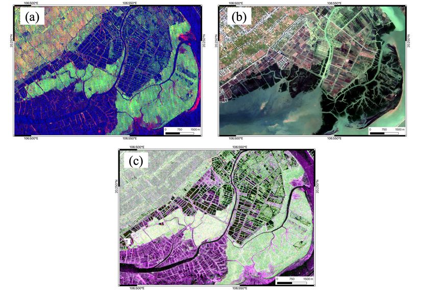
Figure 5. Probability maps of (a) Sonneratia caseolaris (SC), (b) Kandelia obovata (KO), (c) Aegiceras
corniculatum (AC), (d) Rhizophora stylosa (RS), (e) Avicennia marina (AM) generated by the best
performance (OA: 62.44%, AA: 51.90%) using the specialized algorithm with BFGS optimization
(SA-BFGS) and the combination of spectral bands, vegetation indices of Sentinel-2, and four polarization
channels of Gaofen-3, which is short for S2+VIs+GF(4) in the manuscript.
Table 6. Accuracy assessment on the additional 71 plots with different combinations of
multiple-source datasets.
Class No. Samples S2+VIs S1+S2+VIs S2+VIs+GF (4) S2+VIs+GF (All) S1+S2+VIs+GF (All)
2 63 47.62 44.44 50.79 53.97 47.61
3 32 6.25 53.13 56.25 62.50 50.00
4 10 60.00 60.00 60.00 60.00 60.00
5 4 25.00 25.00 25.00 25.00 25.00
2-1 25 92.00 72.00 80.00 64.00 64.00
2-3-1 4 25.00 25.00 25.00 25.00 25.00
2-4 63 36.51 42.85 63.49 52.38 49.20
3-1 79 64.56 60.76 68.35 63.29 60.76
3-2 110 34.55 33.64 38.18 36.36 31.82
Overall accuracy (OA) 44.87 46.66 62.44 58.50 53.36
Average accuracy (AA) 43.49 46.31 51.90 49.19 45.94Remote Sens. 2020, 12, 3834 12 of 17
4. Discussion
4.1. Contribution from the Full-Polarimetric SAR
Mangrove mapping with the combination of optical and SAR datasets has been reported by
previous studies [1,21,27] and few studies have investigated the classification performance with
full-pol SAR (e.g., RADARSAT-2 and ALOS-PALSAR-2) [57,58].
In this work, the complementary role of full-polarimetric GF-3 SAR towards optical data
was tested and assessed for the improvement of mangrove tree species probabilistic mapping.
As we expected, the OAs were improved from 44.87% (S2+VIs) to 46.66% (S2+VIs+S1) and 62.44%
(S2+VIs+GF-3 (4)), while the AAs was improved from 43.49%(S2+VIs) to 46.31% (S2+VIs+S1) and
52.90% (S2+VIs+GF-3 (4)). This improvement can be further explained from the individual accuracies
over different kinds of tree species, showing that GF-3 full-pol SAR may improve the identification
capability of not only the pure types but also the mixed combinations when compared to the dual-pol
SAR. Pauli and Krogager decomposition were included; the classification accuracies of the pure types
of mangrove tree specifies are improved. In future studies, we will compare the performance of L-band
and C-band full-pol SAR and investigate the potential joint use of multifrequency full-pol SAR.
4.2. Factors Affecting Accuracy Assessment
In a real case, very limited reference samples are typical. Collecting many samples under
mangrove ecosystems is extremely difficult, time-consuming, and costly. In this study, only 55 samples
with the probabilities collected by the field survey were used for the training, and the additional
71 sample sites (390 samples) were used for the validation. From a statistical point of view,
this very limited training sample size may decrease reliability. In this work, the classification
performance derived from the combined full-pol GF-3 SAR and optical (S2+VIs) using SA-BFGS
are significantly better than others from only optical and the combined dual-pol SAR and optical with
all applied method.
In machine learning community, active learning and semi-supervised learning are often adopted
to deal with limited training samples. There have been a few attempts to use semi-supervised learning
technique for the mangrove mapping. For instance, Silva et al. [59] proposed to use cost-sensitive
and semi-supervised learning to classify mangrove in Saloum estuary, Senegal, from Landsat imagery.
Weinstein et al. [60] developed semi-supervised deep learning neural networks to detect individual
tree from Airborne RGB images. In the future, we may consider including active learning and
semi-supervised learning to further improve the performance.
4.3. Investigations about Combinations and Methods
The accurate assessment for the spatial distribution of mangrove communities, which consisted
of mixed species, particularly small and shrubs patches, is still a challenging task. In this work,
we investigate and compare the different combination of full-pol SAR, dual-pol SAR and optical data
for probabilistic mangrove mapping.
Two advantages need to be considered. First, regarding the SAR datasets, more and more free
public SAR datasets (e.g., Sentinel-1) are used to increasing the accuracy of mangrove mapping, full-pol
GF-3 datasets are used in this work. Experimental results indicated better performance using full-pol
SAR rather than dual-pol SAR because full-pol SAR could provide more informative features to classify
the different dominant or mixed tree species.
Second, regarding the methodology, most studies worked on mangrove species mapping using
medium resolution images is a pixel-wise method. Due to limited spatial resolution, the mixed tree
species in one pixel often exist. Traditionally the most used approach to deal with the mixed pixel
is the sub-pixel analysis or spectral unmixing [15,34]. In all existing spectral unmixing or sub-pixel
methods, the “pure” pixel should be found. Contrary to these methods, we employed the LDL
methods, which do not need the “pure” pixel and use the probabilistic as the input. We expected thatRemote Sens. 2020, 12, 3834 13 of 17
it could be more useful than the pixel-wise classifier to generate the probabilistic classification maps.
More specifically, three typical kinds of methods were compared: problem transformations (PT-Bayes
and PT-SVM), algorithm adaptation (AA-kNN and AA-BPNN), and specialized algorithm (SA-IIS and
SA-BFGS). As observed from the experiments, the SA methods are better than those of other methods
by considering the accuracy of individual and mixed tree species. When including the full-pol SAR
datasets, the accuracy is further improved.
4.4. Limitation of This Study
Mangroves distribution mapping can be divided into two parts: extent mapping (mangroves
or non-mangroves) and species distribution mapping [5]. Extent mapping can be done by coarse
or medium resolution remote-sensing datasets, such as Landsat and Sentinel, while mangrove tree
species mapping should be obtained from high-spatial-resolution datasets, including IKONOS. Now,
all the studies of mangrove tree species mapping are conducted in a local scale, the species distribution
at continental or global scale is missing.
In this work, we attempt to use LDL methods to produce probability mapping of mangrove tree
species with multi-source datasets. The results encourage us to further extend LDL to large-scale
mapping. However, the main limitation of this study is the very limited training samples with
probabilities. LDL methods require very accurate training samples.
5. Conclusions
This is the first study attempted to investigate the potential of the combined optical and
full-polarimetric SAR remote-sensing data for mapping probabilities of mangrove communities
including mixed several small mangrove species using the LDL approaches in Xuan Thuy National
park located in North Vietnam. Various combinations of remote-sensing datasets, including Sentinel-1
dual-polarimetric SAR, Sentinel-2 multispectral, and Gaofen-3 full-polarimetric SAR, were investigated.
Then, different types LDL methods were applied to classify the mangrove tree species. Experimental
results demonstrated that a combination of spectral bands and all vegetation indices (e.g., NDVI, DVI,
NDI45, RVI, SAVI, IRECI and GNDVI) derived from Sentinel-2 and four polarization channels of
Gaofen-3, which is short for S2+VIs+GF(4), obtained the best performance.
Dual-polarimetric Sentinel-1 SAR data was beneficial to improve the classification of
Aegiceras corniculatum (AC) species. However, the accuracies of the most mixed combination of tree
species, such as the mixture of Sonneratia caseolaris (SC) and Kandelia obovata (KO) species, decreased.
Finally, full-polarimetric SAR datasets tend to improve the accuracy of both pure and mixed types of
tree species. For the method, the best accuracies were obtained by the specialized algorithms (SA) with
Broyden–Fletcher–Goldfarb–Shanno (BFGS) optimization (SA-BFGS). The methods used in this study can
apply for mapping mangrove communities on a large scale due to the efficient computation time (less than
one minute on a computer with Intel Core i7 CPU, 1.30 GHz, and 32 GB of memory). The main reason for
such efficiency is that the method adopts the efficient BFGS optimization method, whose computation is
related to the to the first-order gradient, performing much more efficiently than the standard line search
Newton method (e.g., IIS) based on previous studies [35,61,62]. These findings indicate the reliability
of the LDL method for mapping the probabilistic mangrove species distribution and may provide a
road-map using multi-source datasets and the LDL algorithms in other remote-sensing applications.
Author Contributions: Conceptualization, J.X., N.Y. and T.D.P. conceived and designed the paper. J.X. and T.D.P.
conducted field study and data processing. J.X., N.Y. and T.D.P. wrote and revised the manuscript. All authors
have read and agreed to the published version of the manuscript.
Funding: This research received no external funding.
Acknowledgments: The authors would like to thank the China National Space Administration (CNSA) and
European Space Agency (ESA) for providing the GF-3 and Sentinel datasets, respectively. The authors would like
to thank Miss Thuy Thi Phuong Vu from Forest Inventory and Planning Institute (FIPI), Ministry of Agriculture
and Rural Development (MARD), Vietnam, to provide the reference mangrove base map.Remote Sens. 2020, 12, 3834 14 of 17
Conflicts of Interest: The authors declare no conflict of interest.
References
1. Zhang, H.; Wang, T.; Liu, M.; Jia, M.; Lin, H.; Chu, L.M.; Devlin, A.T. Potential of Combining Optical
and Dual Polarimetric SAR Data for Improving Mangrove Species Discrimination Using Rotation Forest.
Remote Sens. 2018, 10, 467. [CrossRef]
2. Wang, D.; Wan, B.; Qiu, P.; Su, Y.; Guo, Q.; Wang, R.; Sun, F.; Wu, X. Evaluating the Performance of Sentinel-2,
Landsat 8 and Pléiades-1 in Mapping Mangrove Extent and Species. Remote Sens. 2018, 10, 1468. [CrossRef]
3. Künzer, C.; Bluemel, A.; Gebhardt, S.; Quoc, T.V.; Dech, S. Remote Sensing of Mangrove Ecosystems:
A Review. Remote Sens. 2011, 3, 878–928. [CrossRef]
4. Ahmed, N.; Glaser, M. Coastal aquaculture, mangrove deforestation and blue carbon emissions: Is REDD+ a
solution? Mar. Policy 2016, 66, 58–66. [CrossRef]
5. Wang, L.; Jia, M.; Yin, D.; Tian, J. A review of remote sensing for mangrove forests: 1956–2018.
Remote Sens. Environ. 2019, 231, 111223. [CrossRef]
6. Pham, T.D.; Xia, J.; Ha, N.T.; Bui, D.T.; Le, N.N.; Takeuchi, W. A Review of Remote Sensing Approaches for
Monitoring Blue Carbon Ecosystems: Mangroves, Seagrasses and Salt Marshes during 2010–2018. Sensors
2019, 19, 1933. [CrossRef] [PubMed]
7. Wan, L.; Zhang, H.; Liu, M.; Lin, Y.; Lin, H. Early Monitoring of Exotic Mangrove Sonneratia in Hong Kong
Using Deep Convolutional Network at Half-Meter Resolution. IEEE Geosci. Remote Sens. Lett. 2020, in press.
[CrossRef]
8. He, Z.; Shi, Q.; Liu, K.; Cao, J.; Zhan, W.; Cao, B. Object-Oriented Mangrove Species Classification Using
Hyperspectral Data and 3-D Siamese Residual Network. IEEE Geosci. Remote Sens. Lett. 2020, in press.
[CrossRef]
9. Chakravortty, S.; Li, J.; Plaza, A. A Technique for Subpixel Analysis of Dynamic Mangrove Ecosystems With
Time-Series Hyperspectral Image Data. IEEE J. Sel. Top. Appl. Earth Obs. Remote Sens. 2018, 11, 1244–1252.
[CrossRef]
10. Jia, M.; Wang, Z.; Zhang, Y.; Ren, C.; Song, K. Landsat-Based Estimation of Mangrove Forest Loss and
Restoration in Guangxi Province, China, Influenced by Human and Natural Factors. IEEE J. Sel. Top. Appl.
Earth Obs. Remote Sens. 2015, 8, 311–323. [CrossRef]
11. Viennois, G.; Proisy, C.; Féret, J.; Prosperi, J.; Sidik, F.; Suhardjono; Rahmania, R.; Longépé, N.; Germain,
O.; Gaspar, P. Multitemporal Analysis of High-Spatial-Resolution Optical Satellite Imagery for Mangrove
Species Mapping in Bali, Indonesia. IEEE J. Sel. Top. Appl. Earth Obs. Remote Sens. 2016, 9, 3680–3686.
[CrossRef]
12. Son, N.; Chen, C.; Chang, N.; Chen, C.; Chang, L.; Thanh, B. Mangrove Mapping and Change Detection in
Ca Mau Peninsula, Vietnam, Using Landsat Data and Object-Based Image Analysis. IEEE J. Sel. Top. Appl.
Earth Obs. Remote Sens. 2015, 8, 503–510. [CrossRef]
13. Wan, L.; Lin, Y.; Zhang, H.; Wang, F.; Liu, M.; Lin, H. GF-5 Hyperspectral Data for Species Mapping of
Mangrove in Mai Po, Hong Kong. Remote Sens. 2020, 12, 656. [CrossRef]
14. McCarthy, M.J.; Jessen, B.; Barry, M.J.; Figueroa, M.; McIntosh, J.; Murray, T.; Schmid, J.; Muller-Karger, F.E.
Automated High-Resolution Time Series Mapping of Mangrove Forests Damaged by Hurricane Irma in
Southwest Florida. Remote Sens. 2020, 12, 1740. [CrossRef]
15. Taureau, F.; Robin, M.; Proisy, C.; Fromard, F.; Imbert, D.; Debaine, F. Mapping the Mangrove Forest Canopy
Using Spectral Unmixing of Very High Spatial Resolution Satellite Images. Remote Sens. 2019, 11, 367.
[CrossRef]
16. Individual mangrove tree measurement using UAV-based LiDAR data: Possibilities and challenges.
Remote Sens. Environ. 2019, 223, 34–49. [CrossRef]
17. Pham, T.D.; Yokoya, N.; Xia, J.; Ha, N.T.; Le, N.N.; Nguyen, T.T.T.; Dao, T.H.; Vu, T.T.P.; Pham, T.D.;
Takeuchi, W. Comparison of Machine Learning Methods for Estimating Mangrove Above-Ground Biomass
Using Multiple Source Remote Sensing Data in the Red River Delta Biosphere Reserve, Vietnam. Remote Sens.
2020, 12, 1334. [CrossRef]Remote Sens. 2020, 12, 3834 15 of 17
18. Pham, T.D.; Yokoya, N.; Bui, D.T.; Yoshino, K.; Friess, D.A. Remote Sensing Approaches for Monitoring
Mangrove Species, Structure, and Biomass: Opportunities and Challenges. Remote Sens. 2019, 11, 230.
[CrossRef]
19. Hamdan, O.; Khali Aziz, H.; Mohd Hasmadi, I. L-band ALOS PALSAR for biomass estimation of Matang
Mangroves, Malaysia. Remote Sens. Environ. 2014, 155, 69–78. [CrossRef]
20. Kovacs, J.M.; Vandenberg, C.V.; Wang, J.; Flores-Verdugo, F. The Use of Multipolarized Spaceborne SAR
Backscatter for Monitoring the Health of a Degraded Mangrove Forest. J. Coast. Res. 2008, 241, 248–254.
[CrossRef]
21. Pham, T.D.; Yoshino, K.; Kaida, N. Monitoring Mangrove Forest Changes in Cat Ba Biosphere Reserve Using
ALOS PALSAR Imagery and a GIS-Based Support Vector Machine Algorithm. In Advances and Applications
in Geospatial Technology and Earth Resources; Tien Bui, D., Ngoc Do, A., Bui, H.B., Hoang, N.D., Eds.; Springer
International Publishing: Cham, Switzerland, 2018; pp. 103–118.
22. Mougin, E.; Proisy, C.; Marty, G.; Fromard, F.; Puig, H.; Betoulle, J.L.; Rudant, J.P. Multifrequency and
multipolarization radar backscattering from mangrove forests. IEEE Trans. Geosci. Remote Sens. 1999,
37, 94–102. [CrossRef]
23. Proisy, C. Interpretation of Polarimetric Radar Signatures of Mangrove Forests. Remote Sens. Environ. 2000,
71, 56–66. [CrossRef]
24. Zhang, H.; Xu, R. Exploring the optimal integration levels between SAR and optical data for better urban
land cover mapping in the Pearl River Delta. Int. J. Appl. Earth Obs. Geoinf. 2018, 64, 87–95. [CrossRef]
25. Zhang, H.; Lin, H.; Li, Y.; Zhang, Y.; Fang, C. Mapping urban impervious surface with dual-polarimetric
SAR data: An improved method. Landsc. Urban Plan. 2016, 151, 55–63. [CrossRef]
26. Souza, P.; Paradella, W. Use of Radarsat-1 fine mode and Landsat-5 TM selective principal component
analysis for geomorphological mapping in a macrotidal mangrove coast in the amazon region.
Can. J. Remote Sens. 2005, 31, 214–224. [CrossRef]
27. Wong, F.K.K.; Fung, T. Combining Hyperspectral and Radar Imagery for Mangrove Leaf Area Index
Modeling. Photogramm. Eng. Remote Sens. 2013, 79, 479–490. [CrossRef]
28. Wong, F.K.K.; Fung, T. Combining EO-1 Hyperion and Envisat ASAR data for mangrove species classification in
Mai Po Ramsar Site, Hong Kong. Int. J. Remote Sens. 2014, 35, 7828–7856. [CrossRef]
29. Zhang, X.; Treitz, P.M.; Chen, D.; Quan, C.; Shi, L.; Li, X. Mapping mangrove forests using multi-tidal
remotely-sensed data and a decision-tree-based procedure. Int. J. Appl. Earth Obs. Geoinf. 2017, 62, 201–214.
[CrossRef]
30. Xu, L.; Zhang, H.; Wang, C.; Fu, Q. Classification of Chinese GaoFen-3 fully-polarimetric SAR images: Initial
results. In Proceedings of the 2017 Progress in Electromagnetics Research Symposium—Fall (PIERS-FALL),
Singapore, 19–22 November 2017; pp. 700–705.
31. Liu, M.; Li, H.; Li, L.; Man, W.; Jia, M.; Wang, Z.; Lu, C. Monitoring the Invasion of Spartina alterniflora
Using Multi-source High-resolution Imagery in the Zhangjiang Estuary, China. Remote Sens. 2017, 9, 539.
[CrossRef]
32. Peng, L.; Liu, K.; Cao, J.; Zhu, Y.; Li, F.; Liu, L. Combining GF-2 and RapidEye satellite data for mapping
mangrove species using ensemble machine-learning methods. Int. J. Remote Sens. 2020, 41, 813–838.
[CrossRef]
33. Zhu, Y.; Liu, K.W.; Myint, S.; Du, Z.; Li, Y.; Cao, J.; Liu, L.; Wu, Z. Integration of GF2 Optical, GF3 SAR,
and UAV Data for Estimating Aboveground Biomass of China’s Largest Artificially Planted Mangroves.
Remote Sens. 2020, 12, 2039. [CrossRef]
34. Kamal, M.; Phinn, S. Hyperspectral Data for Mangrove Species Mapping: A Comparison of Pixel-Based and
Object-Based Approach. Remote Sens. 2011, 3, 2222–2242. [CrossRef]
35. Geng, X. Label Distribution Learning. IEEE Trans. Knowl. Data Eng. 2016, 28, 1734–1748. [CrossRef]
36. Geng, X.; Yin, C.; Zhou, Z.H. Facial Age Estimation by Learning from Label Distributions. IEEE Trans.
Pattern Anal. Mach. Intell. 2013, 35, 2401–2412. [CrossRef] [PubMed]
37. Geng, X.; Xia, Y. Head Pose Estimation Based on Multivariate Label Distribution; CVPR; IEEE Computer Society:
Columbus, OH, USA, 2014; pp. 1837–1842.Remote Sens. 2020, 12, 3834 16 of 17
38. Zhou, Y.; Xue, H.; Geng, X. Emotion Distribution Recognition from Facial Expressions. In ACM Multimedia;
Zhou, X., Smeaton, A.F., Tian, Q., Bulterman, D.C.A., Shen, H.T., Mayer-Patel, K., Yan, S., Eds.; ACM:
Brisbane, Australia, 2015; pp. 1247–1250.
39. Curnick, D.J.; Pettorelli, N.; Amir, A.A.; Balke, T.; Barbier, E.B.; Crooks, S.; Dahdouh-Guebas, F.; Duncan, C.;
Endsor, C.; Friess, D.A.; et al. The value of small mangrove patches. Science 2019, 363, 239. [PubMed]
40. Veettil, B.K.; Ward, R.D.; Quang, N.X.; Trang, N.T.T.; Giang, T.H. Mangroves of Vietnam: Historical
development, current state of research and future threats. Estuar. Coast. Shelf Sci. 2019, 218, 212–236.
[CrossRef]
41. Nguyen, T.T.N.; Tran, H.C.; Ho, T.M.H.; Burny, P.; Lebailly, P. Dynamics of Farming Systems under the
Context of Coastal Zone Development: The Case of Xuan Thuy National Park, Vietnam. Agriculture 2019,
9, 138. [CrossRef]
42. Rouse, J.W.J.; Haas, R.H.; Schell, J.A.; Deering, D.W. Monitoring Vegetation Systems in the Great Plains with Erts;
NASA Special Publication: Greenbelt, MD, USA, 1974; Volume 351, p. 309.
43. Tucker, C. Red and photographic infrared linear combinations for monitoring vegetation.
Remote Sens. Environ. 1979, 8, 127–150. [CrossRef]
44. Delegido, J.; Verrelst, J.; Alonso, L.; Moreno, J.F. Evaluation of Sentinel-2 Red-Edge Bands for Empirical
Estimation of Green LAI and Chlorophyll Content. Sensors 2011, 11, 7063–7081. [CrossRef]
45. Blackburn, G.A. Quantifying Chlorophylls and Caroteniods at Leaf and Canopy Scales: An Evaluation of Some
Hyperspectral Approaches. Remote Sens. Environ. 1998, 66, 273–285. [CrossRef]
46. Huete, A. A soil-adjusted vegetation index (SAVI). Remote Sens. Environ. 1988, 25, 295–309. [CrossRef]
47. Frampton, W.J.; Dash, J.; Watmough, G.; Milton, E.J. Evaluating the capabilities of Sentinel-2 for quantitative
estimation of biophysical variables in vegetation. ISPRS J. Photogramm. Remote Sens. 2013, 82, 83–92.
[CrossRef]
48. Daughtry, C.; Walthall, C.; Kim, M.; de Colstoun, E.; McMurtrey, J. Estimating Corn Leaf Chlorophyll
Concentration from Leaf and Canopy Reflectance. Remote Sens. Environ. 2000, 74, 229–239. [CrossRef]
49. Freeman, A.; Durden, S.L. A three-component scattering model for polarimetric SAR data. IEEE Trans.
Geosci. Remote Sens. 1998, 36, 963–973. [CrossRef]
50. Krogager, E.; Boerner, W.M.; Madsen, S. Feature-motivated Sinclair matrix (sphere/diplane/helix)
decomposition and its application to target sorting for land feature classification. In Proceedings of
the SPIE Conference on Wideband Interferometric Sensing and Imaging Polarimetry, San Diego, CA, USA,
1 January 1997.
51. Bayes Classifier. In Encyclopedia of Database Systems; Liu, L., Özsu, M.T., Eds.; Springer: New York, NY, USA,
2009; p. 210.
52. Lin, H.T.; Lin, C.J.; Weng, R.C. A note on Platt’s probabilistic outputs for support vector machines.
Mach. Learn. 2007, 68, 267–276. [CrossRef]
53. Xue, D.; Hong, Z.; Guo, S.; Gao, L.; Wu, L.; Zheng, J.; Zhao, N. Personality Recognition on Social Media With
Label Distribution Learning. IEEE Access 2017, 5, 13478–13488. [CrossRef]
54. Miller, D.J.; Zhang, Y.; Kesidis, G. Decision Aggregation in Distributed Classification by a Transductive
Extension of Maximum Entropy/Improved Iterative Scaling. EURASIP J. Adv. Signal Process. 2008, 2008,
674974. [CrossRef]
55. Bazaraa, M.S.; Shetty, C.M. Nonlinear Programming: Theory and Algorithms; Wiley: New York, NY, USA, 1979.
56. Kearns, M.; Ron, D. Algorithmic stability and sanity-check bounds for leave-one-out cross-validation.
Neural Comput. 1999, 11, 1427–1453. [CrossRef]
57. Zhen, J.; Liao, J.; Shen, G. Mapping Mangrove Forests of Dongzhaigang Nature Reserve in China Using
Landsat 8 and Radarsat-2 Polarimetric SAR Data. Sensors 2018, 18, 4012. [CrossRef]
58. Ferrentino, E.; Nunziata, F.; Zhang, H.; Migliaccio, M. On the Ability of PolSAR Measurements to
Discriminate Among Mangrove Species. IEEE J. Sel. Top. Appl. Earth Obs. Remote Sens. 2020, 13, 2729–2737.
[CrossRef]
59. Silva, J.; Bacao, F.; Caetano, M. Specific Land Cover Class Mapping by Semi-Supervised Weighted Support
Vector Machines. Remote Sens. 2017, 9, 181. [CrossRef]
60. Weinstein, B.G.; Marconi, S.; Bohlman, S.; Zare, A.; White, E. Individual Tree-Crown Detection in RGB
Imagery Using Semi-Supervised Deep Learning Neural Networks. Remote Sens. 2019, 11, 1309. [CrossRef]Remote Sens. 2020, 12, 3834 17 of 17
61. Malouf, R. A Comparison of Algorithms for Maximum Entropy Parameter Estimation. In Proceedings of
the Sixth Conference on Natural Language Learning (CoNLL-2002), Taipei, Taiwan, 21 August–1 September
2002; Roth, D., van den Bosch, A., Eds.; ACL: Stroudsburg, PA, USA, 2002.
62. Nocedal, J.; Wright, S.J. Numerical Optimization, 2nd ed.; Springer: New York, NY, USA, 2006.
Publisher’s Note: MDPI stays neutral with regard to jurisdictional claims in published maps and institutional
affiliations.
c 2020 by the authors. Licensee MDPI, Basel, Switzerland. This article is an open access
article distributed under the terms and conditions of the Creative Commons Attribution
(CC BY) license (http://creativecommons.org/licenses/by/4.0/).You can also read