Methodology for deriving the telescope focus function and its uncertainty for a heterodyne pulsed Doppler lidar
←
→
Page content transcription
If your browser does not render page correctly, please read the page content below
Atmos. Meas. Tech., 13, 2849–2863, 2020
https://doi.org/10.5194/amt-13-2849-2020
© Author(s) 2020. This work is distributed under
the Creative Commons Attribution 4.0 License.

Methodology for deriving the telescope focus function and its
uncertainty for a heterodyne pulsed Doppler lidar
Pyry Pentikäinen1 , Ewan James O’Connor2,3 , Antti Juhani Manninen2 , and Pablo Ortiz-Amezcua4,5
1 Institute
          for Atmospheric and Earth System Research/Physics, Faculty of Science, University of Helsinki, Helsinki, Finland
2 FinnishMeteorological Institute, Helsinki, Finland
3 Department of Meteorology, University of Reading, Reading, UK
4 Andalusian Institute for Earth System Research (IISTA-CEAMA), 18006 Granada, Spain
5 Department of Applied Physics, University of Granada, 18071 Granada, Spain

Correspondence: Pyry Pentikäinen (pyry.pentikainen@helsinki.fi)

Received: 21 December 2019 – Discussion started: 9 January 2020
Revised: 9 April 2020 – Accepted: 27 April 2020 – Published: 29 May 2020

Abstract. Doppler lidars provide two measured parame-            1   Introduction
ters, radial velocity and signal-to-noise ratio, from which
winds and turbulent properties are routinely derived. Atten-
uated backscatter, which gives quantitative information on       Coherent Doppler lidar systems are capable of providing ac-
aerosols, clouds, and precipitation in the atmosphere, can       curate radial Doppler velocities at high temporal and spatial
be used in conjunction with the winds and turbulent prop-        resolution and have been employed across a wide range of
erties to create a sophisticated classification of the state     scientific and operational fields. Meteorological applications
of the atmospheric boundary layer. Calculating attenuated        include the retrieval of turbulent properties to determine the
backscatter from the signal-to-noise ratio requires accurate     strength, location, and source of mixing in the atmospheric
knowledge of the telescope focus function, which is usu-         boundary layer and, with many systems having scanning ca-
ally unavailable. Inaccurate assumptions of the telescope fo-    pability, the retrieval of winds. Information on the targets
cus function can significantly deform attenuated backscatter     responsible for the radial Doppler velocities measured by
profiles, even if the instrument is focused at infinity. Here,   the Doppler lidar (e.g. aerosol, cloud, precipitation) would
we present a methodology for deriving the telescope focus        greatly aid the interpretation of both the velocities and the
function using a co-located ceilometer for pulsed heterodyne     products derived from them, but this requires quantitative use
Doppler lidars. The method was tested with Halo Photonics        of the signal power received by the instrument.
StreamLine and StreamLine XR Doppler lidars but should              The performance of a Doppler lidar depends on the signal-
also be applicable to other pulsed heterodyne Doppler lidar      to-noise ratio, SNR, of the system, as SNR determines the
systems. The method derives two parameters of the telescope      radial velocity uncertainty (Rye and Hardesty, 1993; Pear-
focus function, the effective beam diameter and the effec-       son et al., 2009). The outgoing laser beam can be focused to
tive focal length of the telescope. Additionally, the method     improve the SNR at ranges close to the focal length (Pearson
provides uncertainty estimates for the retrieved attenuated      et al., 2002), and this is often used to improve the Doppler li-
backscatter profile arising from uncertainties in deriving the   dar velocity data quality and data availability, particularly in
telescope function, together with standard measurement un-       the atmospheric boundary layer. The optimal choice of focus
certainties from the signal-to-noise ratio. The method is best   will depend on the atmospheric conditions at the deployment
suited for locations where the absolute difference in aerosol    location (Hirsikko et al., 2014).
extinction at the ceilometer and Doppler lidar wavelengths is       Knowledge of how the choice of instrument parameters,
small.                                                           such as the effective focal length of the telescope, impacts
                                                                 the SNR profile is necessary in order to obtain profiles of the
                                                                 attenuated backscatter coefficient (Zhao et al., 1990). A com-

Published by Copernicus Publications on behalf of the European Geosciences Union.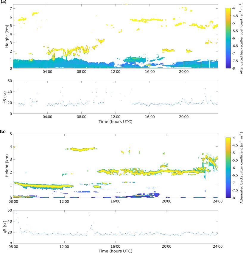
2850                      P. Pentikäinen et al.: Methodology for deriving the telescope focus function and its uncertainty

prehensive overview of the theoretical considerations in de-      retrieve the profile of the attenuated backscatter coefficient
termining the performance of coherent Doppler lidar systems       (Westbrook et al., 2010a; Chouza et al., 2015).
was given by Frehlich and Kavaya (1991), who provided ana-           The theoretical description of the telescope focus func-
lytical expressions for deriving the expected signal measured     tion is outlined in Sect. 2. In Sect. 3, we introduce the in-
by the coherent detector for a given target for a range of in-    struments and the methodology for deriving the parameters
strument configurations, including analytical expressions for     of the telescope focus function experimentally. An iterative
the telescope focus function (also termed coherent respon-        least-squares regression using weighted mean square error
sivity). Most analytical expressions assume ideal Gaussian        (MSE) is used to find the best solution for the telescope fo-
beams, which may not always be appropriate (Hill, 2018);          cus function, where the weights represent the measurement
hence experimental approaches have also been used to deter-       uncertainties in both instruments. The use of long time pe-
mine the impact of beam aberrations (Hu et al., 2013).            riods (1 year or more) also provides an estimate of the un-
   The profile of the attenuated backscatter coefficient has      certainties in the parameters for the telescope focus function,
the potential to be used in real time by weather forecast-        which can then be propagated through to uncertainties in the
ers (Illingworth et al., 2019), as it can be used in the same     retrieved attenuated backscatter coefficients. The methodol-
manner as for ceilometers. This includes the detection of liq-    ogy is applied to different instruments in multiple locations
uid, supercooled-liquid, mixed-phase, and ice clouds (Hogan       in Sect. 4, and the validation of the method is presented in
et al., 2003; Van Tricht et al., 2014; Tonttila et al., 2015),    Sect. 5.
aerosol layer and mixing-height determination (Flentje et al.,
2010; Kotthaus and Grimmond, 2018), and the retrieval of
precipitation parameters (Lolli et al., 2018).                    2     Theory
   In addition to providing velocity estimates for wind and
turbulence, the inclusion of the profile of the attenuated        2.1    Telescope focus function
backscatter coefficient is advantageous for Doppler lidar
boundary layer classification schemes (Tucker et al., 2009;       Following Frehlich and Kavaya (1991), the coherent Doppler
Harvey et al., 2013; Manninen et al., 2018) by enhancing          lidar equation can be expressed as
the discrimination between aerosol, cloud, and precipitation,
                                                                                  ηcE Ae (R) 0
and it can be used for tracking elevated aerosol plumes (Han-     SNR(R) =                  β (R),                           (1)
non et al., 1999). The combination of attenuated backscatter                     2hνB R 2
profiles from coherent Doppler lidars with other profiling in-    where SNR is the signal-to-noise ratio, varying as a func-
struments permits additional retrievals; for example, together    tion of range, R, from the instrument; β 0 is the attenuated
with a ceilometer (Westbrook et al., 2010b), or with a cloud      backscatter coefficient; η is the detector quantum efficiency;
radar (Träumner et al., 2010), it can yield drizzle drop size     c is the speed of light; E is the beam energy; h is Planck’s
and precipitation rate. There is also an advantage to obtaining   constant; ν is the optical frequency; B is the receiver band-
attenuated backscatter and Doppler velocity measurements          width; and Ae is the effective receiver area.
in the same measurement volume, since this will simplify             For a monostatic system emitting a circular Gaussian
the calculation of cloud or aerosol mass fluxes (Engelmann        beam, using a circular aperture, and having matched filters,
et al., 2008).                                                    the effective receiver area is given by Frehlich and Kavaya
   Therefore, an accurate profile of the attenuated backscat-     (1991) and Henderson et al. (2005):
ter coefficient requires confidence in the parameters used to
generate the telescope focus function. The parameters may                             π D2
not be known a priori or may differ from what is assumed,         Ae (R) =     2 2        2  2  ,                    (2)
                                                                                πD          R     D
and incorrect values can result in artefacts and very large bi-           4 1 + 4λR     1 − f + 2ρ 0
ases in the attenuated backscatter coefficient. We present a
methodology for deriving the parameters of the telescope fo-
                                                                  where D is the 1/e2 effective diameter of a Gaussian beam, λ
cus function experimentally from co-located Doppler lidar
                                                                  is the laser wavelength, f is the effective focal length of the
and ceilometer observations, together with the uncertainties
                                                                  telescope for the transmitter and receiver, and ρ0 is a turbu-
in the function parameters. The ceilometer, for which the
                                                                  lent parameter, also termed transverse field coherence length.
overlap function is known, provides our reference attenu-
                                                                     Collecting the range-dependent terms, we obtain a unitless
ated backscatter profiles. This methodology is relevant for
                                                                  telescope focus function:
coherent Doppler lidars designed for meteorological appli-
cations with maximum ranges suitable for observing the full                  Ae (R)
extent of the boundary layer and beyond. Note that a calibra-     Tf (R) =          ,                                        (3)
                                                                              R2
tion constant may still need to be determined and applied af-
ter implementing the calculated telescope focus function to       which is also termed the coherent responsivity (Frehlich and
                                                                  Kavaya, 1991).

Atmos. Meas. Tech., 13, 2849–2863, 2020                                             https://doi.org/10.5194/amt-13-2849-2020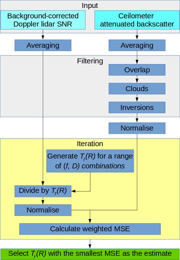
P. Pentikäinen et al.: Methodology for deriving the telescope focus function and its uncertainty                                 2851

  The profile of the attenuated backscatter coefficient is then   Table 1. Halo Photonics StreamLine and StreamLine XR hetero-
obtained by rearranging Eq. (1):                                  dyne Doppler lidar specifications. Values in parentheses refer to the
                                                                  specification of the Doppler lidar during the first period in Darwin.
            2hνB SNR(R)
β 0 (R) =               .                                  (4)
             ηcE Tf (R)                                                     Wavelength               1.5 µm
                                                                            Pulse repetition rate    15 kHz
   Figure 1a shows how Tf (R) depends on the telescope fo-                  Nyquist velocity         19.8 m s−1
cal length, f , and Fig. 1b how Tf (R) depends on D. Both                   Sampling frequency       50 MHz
figures show that the apparent focus – i.e range to the Tf (R)              Points per range gate    10 (16)
maximum – is always closer than f and that decreasing D                     Range resolution         30 m (48 m)
shortens the apparent focus. This makes estimation of the pa-               Pulse duration           0.2 µs
                                                                            Divergence               33 µrad
rameters by eye in Tf (R) prone to errors, since the apparent
                                                                            Antenna                  monostatic fibre-optic
focus cannot be translated into f without knowledge of D.                                            coupled
   Figure 1c shows that even if the telescope is focused at in-
finity, knowledge of the D is essential to derive attenuated
backscatter coefficient profiles. While the gradient of Tf (R)    Table 2. Vaisala CL31 ceilometer specifications.
may be independent of D at the near and far ranges, the rel-
ative magnitude is not, and the potential variation is high in                     Wavelength              910 nm
the range of the profile that is commonly of most interest.                        Pulse repetition rate   5.57 kHz
                                                                                   Range resolution        30 m
2.2    Uncertainty in the attenuated backscatter                                   Lens diameter           14.5 cm
       coefficient                                                                 Divergence              0.75 mrad

Assuming that the parameters Tf (R) and SNR are inde-
pendent, and have uncertainties that can be described as
Gaussian, the relative random uncertainty in the attenuated       are commercially available heterodyne pulsed systems capa-
backscatter coefficient is                                        ble of full hemispheric scanning and operated at a temporal
      q                                                           resolution of 1–2 s (see Table 1). The focus for the Stream-
σβ 0 = σS2 + σT2f ,                                     (5)       Line version can be set by the operator, whereas the Stream-
                                                                  Line XR has the focus set by the manufacturer; however
where σS is the relative uncertainty in the Doppler lidar SNR,    ARM has had some instruments upgraded from their origi-
and σTf is the relative uncertainty in Tf (R). An expression      nal specification.
for deriving σS is given by Manninen et al. (2018), and we           The ceilometer at all sites was a Vaisala CL31 ceilometer,
describe our method for obtaining σTf in Sect. 4.2.               which has a coaxial design and full overlap before 100 m and
                                                                  a temporal resolution of 30 s (more specifications given in
                                                                  Table 2).
3     Application to data

There are three range-dependent unknowns in Eq. (2): f , D,       3.2     Methodology
and ρ0 . We first assume that we can neglect ρ0 and then de-
scribe a method for estimating f and D, together with their       3.2.1    Telescope focus function parameter estimation
uncertainties, which can then be propagated to obtain the un-
certainty in the attenuated backscatter coefficient. The impact   The methodology for deriving the parameters of the tele-
of the ρ0 parameter is discussed in Sect. 4.3.                    scope focus function compares profiles from a co-located
                                                                  Doppler lidar and ceilometer using an iterative least-squares
3.1    Instruments                                                regression to find the best solution. The method follows the
                                                                  process diagram given in Fig. 2.
We used measurements taken from the U.S. Department of               Before input, the Doppler lidar SNR data had a back-
Energy Atmospheric Radiation Measurement (ARM, Mather             ground correction applied to reduce bias (Manninen et al.,
et al., 2016) observatories. We selected five sites with co-      2016). Both ceilometer and Doppler lidar data were aver-
located ceilometer and Doppler lidar instruments: Southern        aged to a common 30 min, 30 m vertical resolution grid. If
Great Plains, US (SGP); tropical west Pacific, Darwin, Aus-       the Doppler lidar vertical resolution was larger than 30 m (as
tralia (Darwin); Barrow, Alaska, US (North Slope of Alaska,       was the case for one period from Darwin), linear interpo-
NSA); Graciosa, Azores (Graciosa); and Ascension Island,          lation was used to match resolutions. After averaging, data
Atlantic, UK (Ascension).                                         below a minimum threshold of −22.2 dB (Manninen et al.,
   The Doppler lidars operated by ARM comprise both Halo          2018) were discarded. The threshold is based on the expected
Photonics StreamLine and StreamLine XR versions. These            noise floor for the instruments considered here (Halo Stream-

https://doi.org/10.5194/amt-13-2849-2020                                             Atmos. Meas. Tech., 13, 2849–2863, 2020
2852 P. Pentikäinen et al.: Methodology for deriving the telescope focus function and its uncertainty Figure 1. Telescope focus functions for (a) varying f with D = 70 mm, (b) varying D with f = 1000 m, and (c) varying D with f being infinity. Line and StreamLine XR) and should probably be modified Due to the wavelength difference between the Doppler li- for different instruments. dar and the ceilometer, it cannot be assumed that the atmo- The data were then filtered to select only those portions spheric backscattering properties are the same at both wave- of the profiles that are considered reliable for comparison. lengths. However, we are only interested in the profile shape, Ceilometer data below 195 m were discarded to ensure that not the absolute values, so profiles from the Doppler lidar only data with full overlap were used. and the ceilometer can be compared as long as they contain Atmos. Meas. Tech., 13, 2849–2863, 2020 https://doi.org/10.5194/amt-13-2849-2020
P. Pentikäinen et al.: Methodology for deriving the telescope focus function and its uncertainty                               2853

                                                                    sulting Doppler lidar attenuated backscatter profiles are nor-
                                                                    malised so that the integral value of the unfiltered portion is
                                                                    unity. We then use a least-squares regression using weighted
                                                                    MSE to find the best solution (smallest MSE), where the
                                                                    weights represent the measurement uncertainties in both in-
                                                                    struments.
                                                                       Collecting results over many profiles results in a bivariate
                                                                    distribution; the peak of this distribution is chosen as the best
                                                                    estimate of f and D, and hence the best estimate of Tf (R),
                                                                    using Eq. (3).

                                                                    3.2.2   Outlier removal

                                                                    Occasionally, data of poor quality pass the filtering step in
                                                                    Fig. 2. The most common issues are noisy ceilometer data
                                                                    and a bias in the Doppler lidar SNR profiles. If not screened,
                                                                    these occasional profiles result in significantly altered Tf (R)
                                                                    estimation. Any noise in the ceilometer data is magnified by
                                                                    the profile length often being relatively short, and hence large
                                                                    uncertainty in even a single range gate can skew the regres-
                                                                    sion. Doppler lidar SNR bias will impact the normalisation
                                                                    process, changing the Tf (R) selected by the method due to
                                                                    the now incorrect profile shape. Due to the non-linearity of
                                                                    the Tf (R) parameter estimation process, these issues result
                                                                    in regression solutions wildly inconsistent with the estimates
Figure 2. Process diagram of the telescope focus function parame-   based on good data. These outliers, which do not fall within
ter estimation.                                                     the normal uncertainty observed in good data, are then re-
                                                                    moved from the bivariate distribution of solutions before cal-
                                                                    culating the uncertainty estimates.
only one type of scatterer, and one which can be assumed               We used the median absolute deviation, MAD (Huber and
to be distributed homogeneously throughout the portion of           Ronchetti, 2009; Leys et al., 2013), to distinguish outliers in
the profile used for comparison. Hence, the portion of a pro-       the bivariate distribution of estimated f and D. MAD can be
file selected for comparison should contain only one aerosol        calculated using
layer, no clouds, and no precipitating hydrometeors.                MAD = b med{|xi − med{xi }|},                                (6)
   We removed clouds by identifying the range gate 150 m
                                                                    where b = 1.4826 when the distribution excluding the out-
below the cloud base detected by the ceilometer and exclud-
                                                                    liers is normal. However, the distribution of f and D may
ing all data beyond this. Elevated aerosol layers and precip-
                                                                    not meet this criterion due to the non-linearity of Tf (R) and
itating hydrometeors were filtered out by identifying layers
                                                                    the computational Tf (R) estimation process. We expect the
using a convolution of the ceilometer profile with a haar-
                                                                    distributions of D and f −2 to be close to normal and will
wavelet to detect changes in the gradient. The base of the
                                                                    use f −2 rather than f to determine outliers. Additionally,
second layer was identified where the gradient was increas-
                                                                    the peak of the bivariate distribution may not always coincide
ing over two range gates, and all data above this were dis-
                                                                    with the medians of the univariate D and f −2 distributions,
carded. This process also eliminates noisy profiles with low
                                                                    and, hence, we use a modified form of Eq. (6),
SNR.
   The Tf (R) parameter estimation is performed on a profile-       MAD = b med{|xi − peak{xi , yi }|}.                          (7)
by-profile basis for each profile where the filtering process          We selected three MADs as the threshold for flagging out-
leaves eight successive range gates present. From Eq. (4),          liers:
dividing the Doppler lidar SNR profile with the appropriate         v
                                                                    u f −2 − med{f −2 } 2  D − med{D } 2
                                                                    u                     !
Tf (R) will generate a Doppler lidar attenuated backscatter         t i                            i         i
                                                                                      i
profile whose shape should match that of the ceilometer at-                                 +                       ≥ 3.     (8)
                                                                            MADf −2                  MADD
tenuated backscatter profile.
   We use a brute-force approach to iterate through a range         Assuming the distribution excluding the outliers to be nor-
of reasonable f and D values, generating a corresponding            mal, three MADs correspond to 3 standard deviations of the
Tf (R) and Doppler lidar attenuated backscatter profile for         underlying distribution. In cases where f is at infinity, all
each combination of values. The ceilometer profile and re-          estimates with a finite f will be flagged as outliers.

https://doi.org/10.5194/amt-13-2849-2020                                              Atmos. Meas. Tech., 13, 2849–2863, 2020
2854 P. Pentikäinen et al.: Methodology for deriving the telescope focus function and its uncertainty Figure 3. Distributions of Tf (R) parameter estimates from (a) Darwin from 21 June 2011 to 22 July 2012, (b) SGP from 1 January 2015 to 2 May 2016, and (c) SGP from 3 May 2016 to 5 June 2017. Outliers filtered using MAD ≥ 3 are marked in black. Atmos. Meas. Tech., 13, 2849–2863, 2020 https://doi.org/10.5194/amt-13-2849-2020
P. Pentikäinen et al.: Methodology for deriving the telescope focus function and its uncertainty 2855
Table 3. Best estimates of f and D together with their uncertainties for Doppler lidars at five ARM sites. Total estimates refers to the number
of ceilometer and Doppler lidar profiles suitable for comparison. Good estimates refers to the number of estimates remaining after outlier
filtering with MAD.
Location Period f D Available profiles Total estimates Good estimates
Ascension 20160906–20170930 550 ± 34 m 25.3 ± 0.5 mm 18 586 62 56
Darwin 20110621–20120722 590 ± 62 m 24.0 ± 0.7 mm 18 988 3684 3528
Darwin 20120921–20140626 545 ± 53 m 25.0 ± 0.8 mm 30 836 5046 4878
Graciosa 20150124–20161114 625 ± 80 m 23.5 ± 0.7 mm 31 124 3737 3161
NSA 20140730–20171231 Infinity 11.8 ± 1.5 mm 56 832 1132 589
SGP 20150101–20160502 440 ± 29 m 25.0 ± 0.7 mm 22 916 9198 8426
SGP 20160503–20170605 425 ± 74 m 14.0 ± 0.4 mm 14 212 5814 5337
4 Results length for this instrument is directly adjustable by any opera-
tor, while the beam diameter is set by the manufacturer and is
4.1 Parameter estimation not modifiable by the operator. We note that the D estimates
are the same for these two periods within the margin of error
We applied the Tf (R) estimation method to Doppler lidars calculated.
at five ARM atmospheric observatories. Figure 3a shows the For the sites and instruments selected here, only the
distribution of f and D calculated for the Doppler lidar oper- Doppler lidar at NSA had f set to infinity. In fact, all Stream-
ating at Darwin in northern Australia between 21 June 2011 Line lidars have D in the vicinity of 25 mm, whereas D for
and 22 July 2012. This Doppler lidar is a StreamLine and the StreamLine XR versions is about half this. Nevertheless,
the distribution of f is positively skewed, as explained in the variation between instruments of the same version is not
Sect. 3.2.2. The distribution displays a slightly wider peak negligible and should be taken into account when calculating
than expected for a normal distribution. Tf (R) and then attenuated backscatter.
Figure 3b shows the distribution of f and D for the The final step to obtain attenuated backscatter profiles is
StreamLine Doppler lidar operating at SGP from 1 Jan- to apply a calibration constant, which can be achieved using
uary 2015 to 2 May 2016. The distribution close to the peak is the liquid cloud calibration method (Westbrook et al., 2010a;
really tight, while the outliers have substantial spread. Many O’Connor et al., 2004).
of the poor estimates responsible for the outlier spread oc- The parameters f and D calculated for period 1 in Dar-
cur during January and February in both years, while for win have been used to derive Tf (R) and the results applied
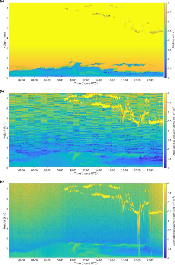
the rest of the period the estimates are remarkably consis- in Fig. 4. This shows the utility of the method, able to pro-
tent. On 3 May 2016 the Doppler lidar at SGP was changed vide reliable Doppler lidar attenuated backscatter profiles in
to a StreamLine XR, and Fig. 3c shows the distribution of Fig. 4b that show no overcorrection below 1 km and dis-
f and D from 3 May 2016 to 5 June 2017. The change in play similar in-cloud values to the ceilometer in Fig. 4c.
instrument version, from StreamLine to StreamLine XR, is It is expected that the aerosol attenuated backscatter coef-
clearly seen in the change in D, whereas the best estimate ficients will differ due to the different scattering properties
for f did not change. However, inspecting the data by eye of aerosol at the different wavelengths; the scattering proper-
would suggest a significantly shorter apparent focus, and the ties of cloud droplets remain similar at the two wavelengths
Tf (R) calculated using the best estimates for f and D also (O’Connor et al., 2004; Westbrook et al., 2010a).
exhibits a significantly shorter apparent focus. Consequently,
the StreamLine XR in SGP has been noted to suffer from 4.2 Uncertainty
poor SNR at the boundary layer top.
The bivariate distributions of f and D show notable vari- A computational method was used to calculate the uncer-
ations in how tight they are around the peak, likely a re- tainty in the estimated Tf (R) as it is a non-linear function
sult of differences in data quality between the instruments. of f and D. We used Monte Carlo simulation (MCS) (Mor-
The best estimates of f and D and their uncertainties for all gan and Henrion, 1990), where a distribution of input values
sites are presented in Table 3. The Doppler lidar measure- is fed into a model, here the effective receiver area Eq. (2),
ments at Darwin were split into two periods, as there was a and the uncertainty is obtained from the distribution of the
2-month break in the measurements between these two pe- output. The input values can be created either from observed
riods. We performed the Tf (R) parameter estimation sepa- statistics or by bootstrapping, i.e. resampling the data. We
rately for both periods. The best estimates from these peri- created three different sets of input values for our MCS:
ods differ from each other, which is expected as some ad-
justments were made to the instrument. The telescope focal
https://doi.org/10.5194/amt-13-2849-2020 Atmos. Meas. Tech., 13, 2849–2863, 20202856 P. Pentikäinen et al.: Methodology for deriving the telescope focus function and its uncertainty Figure 4. (a) Doppler lidar attenuated backscatter coefficient assuming a generic Tf (R), (b) corrected Doppler lidar attenuated backscatter coefficient, and (c) ceilometer attenuated backscatter coefficient, from Darwin on 28 May 2012. Atmos. Meas. Tech., 13, 2849–2863, 2020 https://doi.org/10.5194/amt-13-2849-2020
P. Pentikäinen et al.: Methodology for deriving the telescope focus function and its uncertainty                                    2857

Figure 5. Distributions of the Monte Carlo simulation (MCS) input values used for calculating σTf (R). Values are obtained from (a) resam-
pling, (b) assuming N(f −2 , D), and (c) assuming N(f, D). All distributions contain 5337 samples.

Table 4. σTf (R) uncertainty envelopes generated using MCS with three different sets of input values.

                               Location      Period                  Resampling     N(f −2 , D)     N(f, D)
                               Ascension     20160906–20170930           0.15           0.14            0.16
                               Darwin        20110621–20120722           0.21           0.23            0.25
                               Darwin        20120921–20140626           0.23           0.21            0.28
                               Graciosa      20150124–20161114           0.23           0.19            0.30
                               NSA           20140730–20171231           0.32           0.32            0.30
                               SGP           20150101–20160502           0.20           0.18            0.22
                               SGP           20160503–20170605           0.13           0.13            0.23

  1. Resampling the individual estimates of f and D pro-                Tφ (R), from the best estimate of Tf (R),
     vided directly by the Tf (R) estimation method (i.e. those                    r
     displayed in Fig. 3) after excluding outliers.                                    1
                                                                        σTφ (R) =          6 N (Tφ (R) − Tf (R)),                    (10)
                                                                                     N − 1 i=1 i
  2. Generating the values from the statistics presented in
     Table 3, assuming that D and f −2 are normally dis-                to avoid underestimating the uncertainty resulting from the
     tributed and independent, N (f −2 , D).                            asymmetry in Tφ (R). This also allows us to estimate the im-
                                                                        pact of refractive turbulence on the uncertainty estimate.
  3. Generating the values from statistics presented in Ta-                Examples of the three input parameter distributions are
     ble 3, assuming D and f to be normally distributed and             presented in Fig. 5. Resampling (Fig. 5a) is the most accurate
     independent, N (f, D).                                             method as it does not require assumptions about the parame-
                                                                        ter distributions and their independence. We recommend re-
   For each set of input values, the relative uncertainty in            sampling as the primary method for uncertainty calculation.
Tf (R) is calculated as                                                 Using the N (f −2 , D) distribution (Fig. 5b) produces a set of
                                                                        input values that appear to be a reasonable approximation,
            σTφ (R)                                                     except that the distribution is not as tight around the peak.
σTf (R) =             ,                                        (9)      Using the N (f, D) distribution (Fig. 5c) produces a set of in-
            Tf (R)
                                                                        put values that tend to overemphasise shorter values of f and
where σTφ (R) is expressed in terms of the mean-squared                 underemphasise higher values. We also note that the central
deviation of the MCS-simulated telescope focus function,                bin of the resampled distribution contains 50 % more samples

https://doi.org/10.5194/amt-13-2849-2020                                                   Atmos. Meas. Tech., 13, 2849–2863, 2020
2858 P. Pentikäinen et al.: Methodology for deriving the telescope focus function and its uncertainty
than the central bin of the statistically generated distributions surements are still applicable, but ρ0 (R) must also be calcu-
do. We presume that this is a consequence of the variation in lated or estimated in order to derive the profile of attenuated
SNR not being necessarily normally distributed. backscatter, β 0 (R).
Figure 6a displays σTf (R) for Darwin showing the range
dependence of the uncertainty, with much larger uncertain-
ties for ranges close to either side of the focus (f = 590 m). 5 Validation
The profile of uncertainties obtained with each set of MCS
input values exhibit a similar shape, with N (f −2 , D) being The liquid cloud calibration method (O’Connor et al., 2004;
closer to resampling than N (f, D) in the near field. Westbrook et al., 2010a) is used to determine a calibration
Figure 6b displays σTf (R) for the Doppler lidar at NSA, constant by integrating attenuated backscatter profiles con-
which has f set to infinity; therefore σTf (R) is only depen- taining fully attenuating liquid clouds, which have a well-
dent on the uncertainty in D. Note the reduced uncertain- constrained apparent lidar ratio, ηS, where η is a multiple
ties around 200–400 m, which are expected when examining scattering factor and S is the lidar ratio. In the absence of
Fig. 1c. multiple scattering, ηS can be assumed to be independent of
The largest value of σTf (R) provides the uncertainty enve- the height of the cloud.
lope value for each site, which is presented in Table 4. Re- This calibration method can be used to evaluate the esti-
sampling provides values ranging from 0.12 for the updated mated Tf (R) for Doppler lidar by checking whether the at-
instrument at SGP to 0.32 at NSA. MCS values created us- tenuated backscatter profiles obtained for the Doppler lidar
ing N (f −2 , D) provided similar values, whereas MCS using after applying Tf (R) indeed provide similar ηS values for liq-
N(f, D) often provided much larger uncertainties. uid clouds at different heights.
Figure 8 shows examples of Doppler lidar attenuated
4.3 Impact of refractive turbulence backscatter profiles after calibration and the derived apparent
lidar ratio at two sites, Darwin and NSA. These sites have dif-
So far we have neglected the potential impact of turbulence ferent values of f : Darwin has f = 590 m and NSA has f set
on Tf (R) arising from the refractive turbulent parameter, ρ0 , to infinity. For both cases, liquid clouds are present through-
in Eq. (2). An expression for ρ0 is given in Frehlich and out the day, with altitudes varying from 2 to 6 km. When fully
Kavaya (1991), attenuating liquid clouds are present, the apparent lidar ratio
−3/5 is close to the expected value of 20 sr, regardless of the height
ZR
of the cloud, thus confirming that the method of estimating
ρ0 (R) = H k 2 Cn 2 (z)(1 − z/R)5/3 dz , (11) Tf (R) is valid.
0
Limitations
where H = 2.914383, k = 2π/λ, and Cn 2 (z) is the refrac-
tive turbulence at range z. We chose three profiles with con- Table 3 shows that the proportion of data that can be used for
stant Cn 2 (z) and a realistic vertical profile based on the most the Tf (R) parameter estimation varies significantly from site
turbulent case presented by Roadcap and Tracy (2009). Fig- to site. Over a third of the available profiles from SGP are
ure 7 shows the impact that these different profiles have on used, whereas only 0.3 % pass the filtering for Ascension.
Tf (R) and the resulting resampling calculation of σTf (R) for The lack of suitable profiles at Ascension is explained by the
two Doppler lidar instruments with different Tf (R). Values almost constant low cloud cover at this site, with very few
of Cn 2 up to 10−14 m−2/3 have negligible impact on Tf (R), profiles having a sufficient number of successive range gates.
and even the realistic profile only showed a slight increase in Data quality is also a limiting factor, so at sites with very
σTf (R) for the instrument with a focus set closer than infin- low aerosol optical depth, AOD, such as NSA, the Doppler
ity. This suggests that the impact of turbulence can be safely lidar SNR decreases so rapidly that again there are few pro-
neglected for low values of Cn 2 , and for most applications, it files having a sufficient number of successive range gates.
can also be neglected when operating in the vertical. Hence, Low AOD also impacts the performance of the ceilometer,
turbulence has no significant impact on the methodology de- with 48 % of the estimates at NSA discarded as outliers even
scribed here for deriving the parameters f and D and their after the initial filtering was performed. While the outlier
uncertainties from vertical profiles but can be included for removal can separate the good and the poor estimates, the
completeness. largest uncertainty in D was at NSA. We attempted to per-
However, it is clear that the turbulent impact should not form the Tf (R) parameter estimation on a Doppler lidar from
be ignored when measuring at low elevation angles close to an ARM campaign in Cape Cod but could not obtain reliable
the horizon, where a profile similar to Cn 2 = 10−13 m−2/3 estimates due to the low SNR of the ceilometer data.
may be possible. Figure 7 shows that such a profile has a The Tf (R) parameter estimation method is suitable only in
major impact on Tf (R), especially in the far range. In these situations where there is minimal difference in atmospheric
cases, the parameters f and D obtained from vertical mea- extinction within the aerosol layer between the two instru-
Atmos. Meas. Tech., 13, 2849–2863, 2020 https://doi.org/10.5194/amt-13-2849-2020P. Pentikäinen et al.: Methodology for deriving the telescope focus function and its uncertainty 2859
Figure 6. Relative telescope focus function uncertainties, σTf (R), generated using MCS with three different sets of input values for (a) Darwin
from 21 June 2011 to 22 July 2012 and (b) NSA from 30 July 2014 to 31 December 2017.
ment wavelengths of 910 and 1500 nm. Using AERONET 6 Conclusions
(Aerosol Robotic Network) AOD measurements co-located
at the ARM atmospheric observatories, the median differ- We have developed a method for deriving the telescope focus
ence in AOD at 870 and 1640 nm varied between 0.016 and function and its uncertainty for pulsed heterodyne Doppler
0.027, which should correspond closely to what might be ex- lidars, and we applied the method to Halo Photonics Stream-
pected for the difference between the ceilometer and Doppler Line and XR Doppler lidars. The method compares pro-
lidar. Very occasional periods of notable AOD differences files of the Doppler lidar SNR to profiles of the attenuated
were observed at some sites, but including these profiles in backscatter coefficient from a co-located ceilometer, produc-
time series extending beyond a year will have negligible im- ing estimates for two parameters of the Tf (R): the effective
pact on the Tf (R) parameter best estimate. However, there focal length for the telescope, f ; and the 1/e2 effective di-
were breaks in the AOD measurements, and some periods ex- ameter of a Gaussian beam, D. This method was developed
periencing a significant differential extinction may have gone because it also provides uncertainties in f , D, and Tf (R),
unnoticed. An additional filter using AERONET AOD mea- which are necessary for quantitative use of the subsequently
surements to remove profiles experiencing significant differ- derived attenuated backscatter profiles. The method can be
ential extinction could be included in Fig. 2 for those sites used to check the manufacturer specifications for these pa-
where this may be an issue. rameters, calculate them if not known, and also check their
stability over time. The method does not necessarily require a
permanently co-located ceilometer as the estimates of f and
D can be made from a short time series with a co-located
https://doi.org/10.5194/amt-13-2849-2020 Atmos. Meas. Tech., 13, 2849–2863, 20202860 P. Pentikäinen et al.: Methodology for deriving the telescope focus function and its uncertainty Figure 7. Impact of turbulent parameter, ρ0 , on the telescope focus function, Tf (R), and relative uncertainties, σTf (R), for different Cn 2 profiles. (a) Selected profiles of Cn 2 with range; (b) Tf (R) and (c) σTf (R) for Darwin from 21 June 2011 to 22 July 2012; (d) Tf (R) and (e) σTf (R) for NSA from 30 July 2014 to 31 December 2017. Atmos. Meas. Tech., 13, 2849–2863, 2020 https://doi.org/10.5194/amt-13-2849-2020
P. Pentikäinen et al.: Methodology for deriving the telescope focus function and its uncertainty                               2861

Figure 8. Doppler lidar attenuated backscatter coefficient and apparent lidar ratio, ηS, from (a) Darwin on 8 May 2012 and (b) NSA on
20 August 2014.

ceilometer; the Doppler lidar can then be moved to another           rived input values assuming a normal distribution. The en-
location without a co-located ceilometer using the Tf (R) es-        velope of relative uncertainties in Tf (R) ranged from 13 %
timated previously, assuming that there has been no modifi-          to 32 % and depended on both the instrument configuration
cation to the instrument parameters.                                 and the instrument location. We also show that, even for a
   The method was applied to data from Doppler lidars with           Doppler lidar with the focus set at infinity, uncertainty re-
different configurations deployed at five ARM sites. Rela-           mains in estimating Tf (R) arising from the uncertainty in D.
tive uncertainties in f for these instruments ranged from 6 %        The method was validated by calculating the apparent lidar
to 17 %, with the median uncertainty being 10 %; the rela-           ratio of fully attenuating liquid clouds from Tf (R) corrected
tive uncertainty in D ranged from 2 % to 12 %, with a me-            profiles of Doppler lidar attenuated backscatter.
dian of 3 %. The uncertainty in Tf (R) was calculated using             The impact of turbulence on Tf (R) was also investigated
Monte Carlo simulation, using three methods to prepare the           and was found to have no significant impact on the methodol-
input values. We recommend the direct resampling method,             ogy described here for deriving the parameters f and D and
but reasonable results were obtained using statistically de-         their uncertainties from vertical profiles. However, the tur-

https://doi.org/10.5194/amt-13-2849-2020                                               Atmos. Meas. Tech., 13, 2849–2863, 2020
2862                        P. Pentikäinen et al.: Methodology for deriving the telescope focus function and its uncertainty

bulent impact should not be ignored when measuring at low             References
elevation angles close to the horizon, as it can modify Tf (R)
considerably, especially in the far range. In these cases, the        CEIL: Atmospheric Radiation Measurement (ARM) user facility,
parameters f and D obtained from vertical measurements                   updated hourly. Ceilometer (CEIL). 2011-06-21 to 2017-12-21,
                                                                         ARM Mobile Facility (ASI) Ascension Island, South Atlantic
are still applicable, but the turbulent contribution to Tf (R)
                                                                         Ocean; AMF1 (M1), Eastern North Atlantic (ENA) Graciosa Is-
should be included when deriving the attenuated backscatter              land, Azores, Portugal (C1), North Slope Alaska (NSA) Cen-
coefficient.                                                             tral Facility, Barrow AK (C1), Southern Great Plains (SGP)
   The Tf (R) estimation method is suitable only for con-                Central Facility, Lamont, OK (C1), Tropical Western Pacific
ditions where the differential extinction at the two wave-               (TWP) Central Facility, Darwin, Australia (C3), compiled by:
lengths of the Doppler lidar and the ceilometer is small,                Morris, V., Flynn, C., and Ermold, B., ARM Data Center,
which can be identified, for example, using AOD from co-                 https://doi.org/10.5439/1181954, 2002.
located AERONET observations.                                         Chouza, F., Reitebuch, O., Groß, S., Rahm, S., Freudenthaler,
                                                                         V., Toledano, C., and Weinzierl, B.: Retrieval of aerosol
                                                                         backscatter and extinction from airborne coherent Doppler
Data availability. The ground-based data used in this article are        wind lidar measurements, Atmos. Meas. Tech., 8, 2909–2926,
generated by the Atmospheric Radiation Measurement (ARM)                 https://doi.org/10.5194/amt-8-2909-2015, 2015.
user facility and are made available from the ARM Data Dis-           DLFPT: Atmospheric Radiation Measurement (ARM) user facil-
covery website as follows: ceilometer data (CEIL, 2002) from             ity, updated hourly. Doppler lidar fixed-pointing (DLFPT). 2011-
https://doi.org/10.5439/1181954 and Doppler lidar data (DLFPT,           06-21 to 2017-12-21, ARM Mobile Facility (ASI) Ascension Is-
2010) from https://doi.org/10.5439/10251850.                             land, South Atlantic Ocean; AMF1 (M1), Eastern North Atlantic
                                                                         (ENA) Graciosa Island, Azores, Portugal (C1), North Slope
                                                                         Alaska (NSA) Central Facility, Barrow AK (C1), Southern Great
                                                                         Plains (SGP) Central Facility, Lamont, OK (C1), Tropical West-
Author contributions. EJO supervised and conceptualised the
                                                                         ern Pacific (TWP) Central Facility, Darwin, Australia (C3), com-
project. PP created the methodology and performed the analysis.
                                                                         piled by: Newsom, R. and Krishnamurthy, R., ARM Data Center,
AJM provided the processed input data. POA and AJM contributed
                                                                         https://doi.org/10.5439/1025185, 2010.
to the development of the methodology. PP and EJO wrote the pa-
                                                                      Engelmann, R., Wandinger, U., Ansmann, A., Müller, D.,
per.
                                                                         Z̆eromskis, E., Althausen, D., and Wehner, B.: Lidar ob-
                                                                         servations of the vertical aerosol flux in the planetary
                                                                         boundary layer, J. Atmos. Ocean. Tech., 25, 1296–1306,
Competing interests. The authors declare that they have no conflict      https://doi.org/10.1175/2007JTECHA967.1, 2008.
of interest.                                                          Flentje, H., Heese, B., Reichardt, J., and Thomas, W.: Aerosol
                                                                         profiling using the ceilometer network of the German Meteo-
                                                                         rological Service, Atmos. Meas. Tech. Discuss., 3, 3643–3673,
Special issue statement. This article is part of the special issue       https://doi.org/10.5194/amtd-3-3643-2010, 2010.
“Tropospheric profiling (ISTP11) (AMT/ACP inter-journal SI)”. It      Frehlich, R. G. and Kavaya, M. J.: Coherent laser radar performance
is a result of the 11th edition of the International Symposium on        for general atmospheric refractive turbulence, Appl. Optics, 30,
Tropospheric Profiling (ISTP), Toulouse, France, 20–24 May 2019.         5325–5352, https://doi.org/10.1364/AO.30.005325, 1991.
                                                                      Hannon, S. M., Thomson, J. A. L., and Smith, D. D.: Plume
                                                                         detection and tracking using Doppler lidar aerosol and wind
Acknowledgements. The Doppler lidar and ceilometer data used in          data, in: Application of Lidar to Current Atmospheric Topics
this study were obtained from the Atmospheric Radiation Measure-         III, edited by: Sedlacek III, A. J. and Fischer, K. W., 3757,
ment (ARM) user facility, managed by the Office of Biological and        28–39, International Society for Optics and Photonics, SPIE,
Environmental Research for the U.S. Department of Energy Office          https://doi.org/10.1117/12.366435, 1999.
of Science.                                                           Harvey, N. J., Hogan, R. J., and Dacre, H. F.: A method to diagnose
                                                                         boundary-layer type using Doppler lidar, Q. J. Roy. Meteor. Soc.,
                                                                         139, 1681–1693, https://doi.org/10.1002/qj.2068, 2013.
Financial support. This research has been supported by the U.S.       Henderson, S. W., Gatt, P., Rees, D., and Huffaker, R. M.: Wind
Department of Energy’s Atmospheric System Research (ASR),                Lidar, in: Laser Remote Sensing, edited by: Fujii, T. and Fukuchi,
an Office of Science, Office of Biological and Environmental             T., 469–722, CRC Taylor and Francis, 2005.
Research (BER) programme (grant no. DE-SC0017338).                    Hill, C.: Coherent focused lidars for Doppler sens-
                                                                         ing of aerosols and wind, Remote Sens., 10, 466,
Open access funding provided by Helsinki University Library.             https://doi.org/10.3390/rs10030466, 2018.
                                                                      Hirsikko, A., O’Connor, E. J., Komppula, M., Korhonen, K.,
                                                                         Pfüller, A., Giannakaki, E., Wood, C. R., Bauer-Pfundstein, M.,
Review statement. This paper was edited by Pauline Martinet and          Poikonen, A., Karppinen, T., Lonka, H., Kurri, M., Heinonen,
reviewed by two anonymous referees.                                      J., Moisseev, D., Asmi, E., Aaltonen, V., Nordbo, A., Rodriguez,
                                                                         E., Lihavainen, H., Laaksonen, A., Lehtinen, K. E. J., Laurila,
                                                                         T., Petäjä, T., Kulmala, M., and Viisanen, Y.: Observing wind,

Atmos. Meas. Tech., 13, 2849–2863, 2020                                                 https://doi.org/10.5194/amt-13-2849-2020
P. Pentikäinen et al.: Methodology for deriving the telescope focus function and its uncertainty 2863
aerosol particles, cloud and precipitation: Finland’s new ground- O’Connor, E. J., Illingworth, A. J., and Hogan, R. J.:
based remote-sensing network, Atmos. Meas. Tech., 7, 1351– A technique for autocalibration of cloud lidar, J. At-
1375, https://doi.org/10.5194/amt-7-1351-2014, 2014. mos. Ocean. Tech., 21, 777–786, https://doi.org/10.1175/1520-
Hogan, R. J., Illingworth, A. J., O’Connor, E. J., and Polares Bap- 0426(2004)0212.0.CO;2, 2004.
tista, J. P. V.: Characteristics of mixed-phase clouds. II: A cli- Pearson, G., Davies, F., and Collier, C.: An analysis of the per-
matology from ground-based lidar, Q. J. Roy. Meteor. Soc., 129, formance of the UFAM pulsed Doppler lidar for observing the
2117–2134, https://doi.org/10.1256/qj.01.209, 2003. boundary layer, J. Atmos. Ocean. Tech., 26, 240–250, 2009.
Hu, Q., Rodrigo, P. J., Iversen, T. F. Q., and Pedersen, Pearson, G. N., Roberts, P. J., Eacock, J. R., and Harris, M.: Anal-
C.: Investigation of spherical aberration effects on co- ysis of the performance of a coherent pulsed fiber lidar for
herent lidar performance, Opt. Express, 21, 25670–25676, aerosol backscatter applications, Appl. Optics, 41, 6442–6450,
https://doi.org/10.1364/OE.21.025670, 2013. https://doi.org/10.1364/AO.41.006442, 2002.
Huber, P. J. and Ronchetti, E.: Robust Statistics, Roadcap, J. R. and Tracy, P.: A preliminary comparison of daylit
chap. 5, 105–123, John Wiley & Sons, Ltd, and night Cn2 profiles measured by thermosonde, Radio Sci., 44,
https://doi.org/10.1002/9780470434697.ch5, 2009. https://doi.org/10.1029/2008RS003921, 2009.
Illingworth, A. J., Cimini, D., Haefele, A., Haeffelin, M., Hervo, Rye, B. J. and Hardesty, R. M.: Discrete spectral peak estimation in
M., Kotthaus, S., Löhnert, U., Martinet, P., Mattis, I., O’Connor, incoherent backscatter heterodyne lidar. I. Spectral accumulation
E. J., and Potthast, R.: How can existing ground-based profiling and the Cramer-Rao lower bound, IEEE T. Geosci. Remote, 31,
instruments improve European weather forecasts?, B. Am. Mete- 16–27, https://doi.org/10.1109/36.210440, 1993.
orol. Soc., 100, 605–619, https://doi.org/10.1175/BAMS-D-17- Tonttila, J., O’Connor, E. J., Hellsten, A., Hirsikko, A., O’Dowd, C.,
0231.1, 2019. Järvinen, H., and Räisänen, P.: Turbulent structure and scaling of
Kotthaus, S. and Grimmond, C. S. B.: Atmospheric boundary-layer the inertial subrange in a stratocumulus-topped boundary layer
characteristics from ceilometer measurements. Part 1: A new observed by a Doppler lidar, Atmos. Chem. Phys., 15, 5873–
method to track mixed layer height and classify clouds, Q. J. Roy. 5885, https://doi.org/10.5194/acp-15-5873-2015, 2015.
Meteor. Soc., 144, 1525–1538, https://doi.org/10.1002/qj.3299, Träumner, K., Handwerker, J., Wieser, A., and Grenzhäuser,
2018. J.: A Synergy Approach to Estimate Properties of Rain-
Leys, C., Ley, C., Klein, O., Bernard, P., and Licata, L.: Detecting drop Size Distributions Using a Doppler Lidar and
outliers: Do not use standard deviation around the mean, use ab- Cloud Radar, J. Atmos. Ocean. Tech., 27, 1095–1100,
solute deviation around the median, J. Exp. Soc. Psychol., 49, https://doi.org/10.1175/2010JTECHA1377.1, 2010.
764–766, https://doi.org/10.1016/j.jesp.2013.03.013, 2013. Tucker, S. C., Senff, C. J., Weickmann, A. M., Brewer, W. A.,
Lolli, S., D’Adderio, L. P., Campbell, J. R., Sicard, M., Wel- Banta, R. M., Sandberg, S. P., Law, D. C., and Hardesty, R. M.:
ton, E. J., Binci, A., Rea, A., Tokay, A., Comerón, A., Barra- Doppler lidar estimation of mixing height using turbulence,
gan, R., Baldasano, J. M., Gonzalez, S., Bech, J., Afflitto, N., shear, and aerosol Profiles, J. Atmos. Ocean. Tech., 26, 673–688,
Lewis, J., and Madonna, F.: Vertically resolved precipitation in- https://doi.org/10.1175/2008JTECHA1157.1, 2009.
tensity retrieved through a synergy between the ground-Based Van Tricht, K., Gorodetskaya, I. V., Lhermitte, S., Turner, D. D.,
NASA MPLNET lidar network measurements, surface disdrom- Schween, J. H., and Van Lipzig, N. P. M.: An improved algorithm
eter datasets and an analytical model solution, Remote Sens., 10, for polar cloud-base detection by ceilometer over the ice sheets,
1102, https://doi.org/10.3390/rs10071102, 2018. Atmos. Meas. Tech., 7, 1153–1167, https://doi.org/10.5194/amt-
Manninen, A. J., O’Connor, E. J., Vakkari, V., and Petäjä, T.: A gen- 7-1153-2014, 2014.
eralised background correction algorithm for a Halo Doppler li- Westbrook, C., Illingworth, A., O’Connor, E., and Hogan, R.:
dar and its application to data from Finland, Atmos. Meas. Tech., Doppler lidar measurements of oriented planar ice crystals
9, 817–827, https://doi.org/10.5194/amt-9-817-2016, 2016. falling from supercooled and glaciated layer clouds, Q. J.
Manninen, A. J., Marke, T., Tuononen, M., and O’Connor, Roy. Meteor. Soc., 136, 260–276, https://doi.org/10.1002/qj.528,
E. J.: Atmospheric boundary layer classification with 2010a.
Doppler lidar, J. Geophys. Res.-Atmos., 123, 8172–8189, Westbrook, C. D., Hogan, R. J., O’Connor, E. J., and Illingworth,
https://doi.org/10.1029/2017JD028169, 2018. A. J.: Estimating drizzle drop size and precipitation rate using
Mather, J. H., Turner, D. D., and Ackerman, T. P.: Scien- two-colour lidar measurements, Atmos. Meas. Tech., 3, 671–
tific maturation of the ARM Program, Meteorol. Monogr., 681, https://doi.org/10.5194/amt-3-671-2010, 2010b.
57, 4.1–4.19, https://doi.org/10.1175/AMSMONOGRAPHS-D- Zhao, Y., Post, M. J., and Hardesty, R. M.: Receiving efficiency of
15-0053.1, 2016. monostatic pulsed coherent lidars. 1: Theory, Appl. Optics, 29,
Morgan, M. G. and Henrion, M.: Uncertainty: A guide to 4111–4119, https://doi.org/10.1364/AO.29.004111, 1990.
dealing with uncertainty in quantitative risk and pol-
icy analysis, 172–219, Cambridge University Press,
https://doi.org/10.1017/CBO9780511840609.009, 1990.
https://doi.org/10.5194/amt-13-2849-2020 Atmos. Meas. Tech., 13, 2849–2863, 2020You can also read