Mapping and Assessment of Tree Roots Using Ground Penetrating Radar with Low-Cost GPS - MDPI
←
→
Page content transcription
If your browser does not render page correctly, please read the page content below
remote sensing
Article
Mapping and Assessment of Tree Roots Using
Ground Penetrating Radar with Low-Cost GPS
Lilong Zou 1, * , Yan Wang 2 , Iraklis Giannakis 1 , Fabio Tosti 1 , Amir M. Alani 1 and
Motoyuki Sato 3
 1    School of Computing and Engineering, University of West London (UWL), London W5 5RF, UK;
      iraklis.giannakis@uwl.ac.uk (I.G.); fabio.tosti@uwl.ac.uk (F.T.); Amir.Alani@uwl.ac.uk (A.M.A.)
 2    Department of Earth and Space Sciences, Southern University of Science and Technology, Shenzhen 518055,
      China; 11930877@mail.sustech.edu.cn
 3    Center for Northeast Asian Studies, Tohoku University, Sendai 9808576, Japan;
      motoyuki.sato.b3@tohoku.ac.jp
 *    Correspondence: lilong.zou@uwl.ac.uk; Tel.: +44-(0)-20-8231-2037

 Received: 17 March 2020; Accepted: 18 April 2020; Published: 20 April 2020

 Abstract: In this paper, we have presented a methodology combining ground penetrating radar
 (GPR) and a low-cost GPS receiver for three-dimensional detection of tree roots. This research aims to
 provide an effective and affordable testing tool to assess the root system of a number of trees. For this
 purpose, a low-cost GPS receiver was used, which recorded the approximate position of each GPR
 track, collected with a 500 MHz RAMAC shielded antenna. A dedicated post-processing methodology
 based on the precise position of the satellite data, satellite clock offsets data, and a local reference
 Global Navigation Satellite System (GNSS) Earth Observation Network System (GEONET) Station
 close to the survey site was developed. Firstly, the positioning information of local GEONET stations
 was used to filter out the errors caused by satellite position error, satellite clock offset, and ionosphere.
 In addition, the advanced Kalman filter was designed to minimise receiver offset and the multipath
 error, in order to obtain a high precision position of each GPR track. Kirchhoff migration considering
 near-field effect was used to identify the three-dimensional distribution of the root. In a later stage, a
 novel processing scheme was used to detect and clearly map the coarse roots of the investigated tree.
 A successful case study is proposed, which supports the following premise: the current scheme is an
 affordable and accurate mapping method of the root system architecture.

 Keywords: tree roots mapping; ground penetrating radar (GPR); low-cost GPS; data processing
 methodology; 3D GPR

1. Introduction
     Environmental issues such as the conservation of natural heritage and ancient trees have become
priority objectives of urgent protection [1,2]. Very limited knowledge is present on how the elements
causing the rapid death of entire forests interact with each other. The quality and distribution of roots
can be used as reliable diagnostic parameters for early tree decline [3–5]. Therefore, if the depth of the
root and its extension to the surrounding area can be estimated, more effective preconditions can be
provided to guide a wide range of research decisions [6].
     Destructive methods can provide accurate mapping of the root systems. Nonetheless, intrusive
approaches are often impossible to implement in the field and time-consuming. In addition, digging
and trenching can affect the surrounding of trees and may cause irreversible damage [7]. Destructive
methods are limited in space and can only provide local information on the tree conditions. Instead,
non-destructive testing (NDT) methods are becoming more and more common in forestry and

Remote Sens. 2020, 12, 1300; doi:10.3390/rs12081300                        www.mdpi.com/journal/remotesensing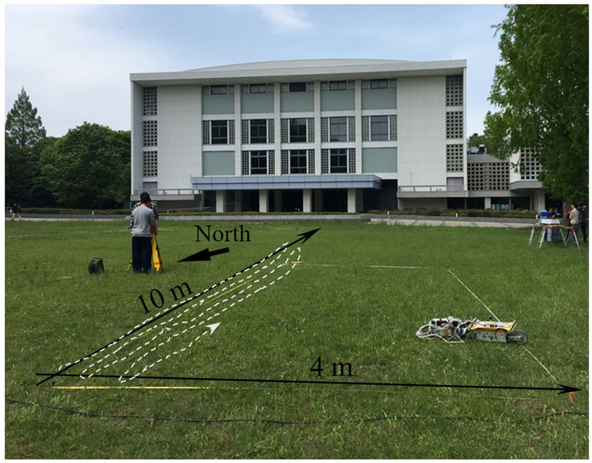
Remote Sens. 2020, 12, 1300                                                                          2 of 16

arboriculture applications due to the high productivity and reliability of the information provided.
Based on the aforementioned factors, GPR technology has been proven to be one of the most effective
NDT tools. GPR is characterized by a high versatility, a fast data collection, and the provision of reliable
results, at relatively limited costs. GPR has been widely used in various disciplines, such as pavement
analysis [8,9], archaeological investigations [10], mine detection [11] and civil and environmental
engineering applications [12]. The application of GPR in forestry sciences is usually related to tree
trunk assessment, root mapping, and the evaluation of the soil-tree interaction. The first application
of GPR in tree root research can be traced back to 1999 [13], referring to the mapping of tree root
systems. Since then, research has focused on the evaluation of the root diameter [14–16] in urban
areas, the functions of the root system architecture such as biomass [17–20], roughness [21–23] and
root mode [24–26].
      In recent years, with the further development of GPR, especially the combination with advanced
positioning systems, it was possible to detect the 3D structure in the subsurface with a 3D full-resolution,
such as in the case of the tree root system presented in [27]. In [27], a 3D GPR system coupled with a
high precision position scheme was used for mapping tree roots. This high-precision framework is
based on three indoor GPS transmitters and uses a laser receiver fixed on the GPR to track the location
of the each GPR trace. At the cost of expensive equipment and time-consuming field measurement,
it can achieve the accuracy of hundreds of microns. In [28], the rotary laser positioning technology
has been applied in 3D GPR measurements. The positioning system enables a centimeter accuracy to
be achieved by using small detectors attached to the GPR antennas. In [29], another high-precision
positioning system, self-tracking total station, was used for 3D GPR field measurements purposes.
The self-tracking total station needs a cable connection, so it is not a flexible in-field application.
Although the wireless communication between GPR and self-tracking total station (TTS) system
was developed to avoid cable connection, the crosstalk effect and the time synchronization required
between the GPR and the positioning system have a significant impact on the data quality of GPR.
Other instruments such as charge-coupled device (CCD) cameras, real-time kinematic GPS (RTK GPS)
and gyroscope can also be used for actual GPR measurements. However, due to the high costs and the
large demand for calculation and operation, the applicability of these methods in real-life applications
is limited.
      Within this context, the aim of this study was to develop a methodology to process the data
acquired by a cost-effective 3D GPR system. Cost-effectiveness is intended in a way that the system has
a low system complexity and a higher efficiency. The methodology is coupled with a set of optimisation
algorithms in order to achieve fast and affordable detection tools fine-tuned for the detection of roots.
      The rest of the paper is divided into five main sections. Section 2 describes the aims and
objectives of this paper. Section 3 introduces the survey site and the data acquisition in the field. This
section also discusses the low-cost GlobalSat GPS Receiver and the B-scan outputs collected in the
measurements. Section 4 presents the data processing methodology that includes the pre-processing
and the post-processing of the tracking position, and the Kirchhoff migration. Section 5 discusses a
novel approach to isolate and highlight the coarse roots of the tree, providing a map about their 3D
distribution. Section 6 summarises the main findings and conclusions of this research.

2. Aims and Objectives
     The main aim of the current research was to provide an effective, economical, and full-resolution
mapping for the assessment of the roots system.
     To that extent, the following objectives were identified: First, to develop an algorithm that could
provide high-precision position information for each GPR trace by a low-cost GPS positioning system.
Second, to develop a novel data-processing approach for achieving 3D full-resolution visualisation of
shallow and deep region tree roots.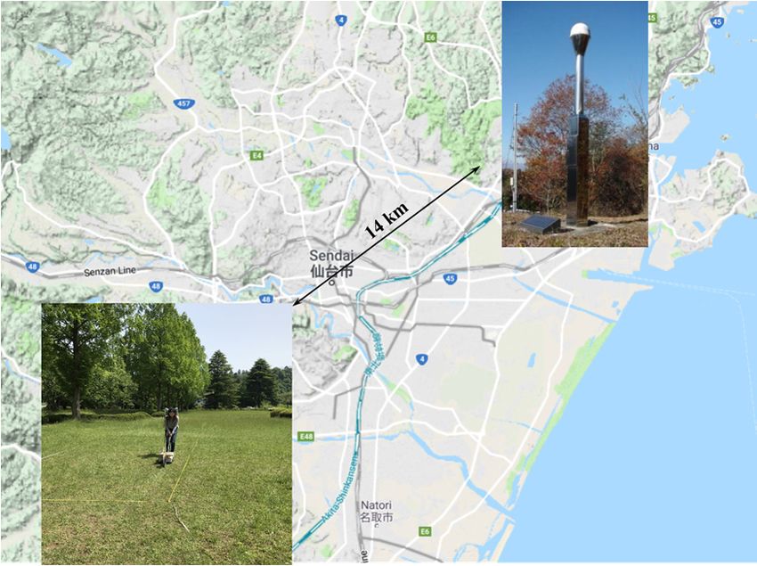
Remote Sens. 2020, 01, x FOR PEER REVIEW 3 of 16
among other international venues and cultural facilities. The site was once the place where the U.S.
Remotemilitary
Sens. 2020,was stationed
12, 1300 after World War II. After that, the Kawauchi Hagi Hall and the surrounding 3 of 16
facilities were built in this area. The survey site was located in a rectangular area measuring 10 m × 4
m in the large open lawn, about 6-m beside the surrounding trees. The latter are typical Metasequoia
3. Survey Site and Data Acquisition
glyptostroboides, with an average diameter at breast height of around 50 cm and a tree height that
can approach
The tree 20 measurements
roots field m. Figure 1awere shows
carriedtheoutscenario of open
over a large the investigated
lawn in front site.
of theMetasequoia
Tohoku
glyptostroboides
University Centennialbelong to a shallow-rooted
Hall–Kawauchi Hagi Hall. species.
The HallThe main roots
is located of trees are
in downtown underdeveloped,
Sendai (Japan)
whereas the lateral roots or adventitious roots grown by radiation are much
among other international venues and cultural facilities. The site was once the place where the longer. Most of the
U.S.roots
are distributed
military was stationed on after
the surface
World ofWartheII.soil.
AfterLateral
that, roots are mainly
the Kawauchi distributed
Hagi Hall andbetween 0.2–1 m, with
the surrounding
some
facilities treebuilt
were roots being
in this exposed
area. to thesite
The survey ground. The white
was located dashed line
in a rectangular areawith an arrow
measuring 10 min ×Figure
4 m 1a
in theindicates
large open thelawn,
investigation
about 6-mdirection
beside the crossing the root
surrounding distribution
trees. The latter that was used
are typical for the data
Metasequoia
collection stage.
glyptostroboides, with an average diameter at breast height of around 50 cm and a tree height that can
approach For 20 m.theFigure
purpose of this
1a shows theinvestigation,
scenario of thea investigated
500 MHz RAMAC shielded glyptostroboides
site. Metasequoia bowtie antenna was
belongemployed. Frequency species.
to a shallow-rooted characteristics
The main of the
rootsantenna
of trees is
aresummarised
underdeveloped,in Table 1. Using
whereas a low-cost
the lateral
rootsGlobalSat GPS receiver
or adventitious (Figure
roots grown by1b) in combination
radiation are muchwith a GPR
longer. Mostsystem,
of the the
rootspositional coordinates
are distributed on of
the surface of the soil. Lateral roots are mainly distributed between 0.2–1 m, with some tree roots beingexact
the moving antenna was able to be recorded in the collected GPR track. In order to obtain the
location
exposed to theofground.
the relevant
The GPR
whitetrace,
dashedthe line
localwith
GEONET station
an arrow and the
in Figure 1aGNSS information
indicates were needed
the investigation
for post-processing
direction crossing the root ofdistribution
the positionthatdatawascollected by the
used for the data
low-cost GPR on
collection the site.
stage.
(a) (b)
Figure 1. (a) 1.
Figure Surveying scenario
(a) Surveying of theofMetasequoia
scenario trees using
the Metasequoia the proposed
trees using 3D GPR
the proposed 3D system. (b) The
GPR system. (b) The
low-cost GlobalSat GPS receiver used in this investigation.
low-cost GlobalSat GPS receiver used in this investigation.
For the purpose
Table of this
1. System investigation,
parameters a 500 MHz
of the RAMAC RAMAC
500 MHz shielded
Shielded bowtie
Antenna antenna
system was
used for employed.
investigation
Frequencypurposes
characteristics
[27]. of the antenna is summarised in Table 1. Using a low-cost GlobalSat GPS
receiver (Figure 1b) in combination with a GPR system, the positional coordinates of the moving
antenna was able to be recorded Parameters
in the collected GPR track. RAMAC 500 MHz
In order Shielded
to obtain Antenna
the exact location
of the relevantLimit
GPRfrequency
trace, the lower than -10 dB:
local GEONET FLow and the GNSS information
station 138 MHz were needed for
post-processing of the
Limit positionhigher
frequency data collected dB:theF low-cost GPR on the 591
than -10 by High
site.MHz
Bandwidthofofthe
Table 1. System parameters −10 dB: B500
RAMAC 453used
MHz Shielded Antenna system
−10 dB MHz for investigation
purposes [27].
Center frequency: FCenter 364 MHz
Parameters
In this study, to make the maximum amountRAMAC
of clear 500 MHz Shielded Antenna
three-dimensional views of the tree roots
and understand how thelower
Limit frequency root than
distributed
−10 dB: F over
Low the subsurface, high-density
138 MHz GPR data acquisitions are
Limit frequency higher than −10 dB: F
usually required. According to [27,30], the sampling
High rate Δ must be equal to or less than the Nyquist
591 MHz
sampling rateBandwidth
∆ alongofthe −10direction
dB: B−10dBof investigation and cross-investigation
453 MHz for the full-resolution
Center frequency: FCenter 364 MHz
3D imaging:
In this study, to make the maximum amount of clear three-dimensional views of the tree roots
and understand how the root distributed over the subsurface, high-density GPR data acquisitions are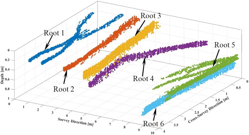
∆      ∆    =                                                       (1)

where         is the main lobe angle of the antenna that was used in the investigation and                             is the
wavelength of the subsurface material. Since the main lobe angle of the GPR antenna used in the near
Remote
field isSens. 2020, 12,
          usually       1300
                     greater    than 60°, the maximum space interval should be equal to or less than4one-                of 16
quarter wavelength of the antenna bandwidth on the subsurface [27].
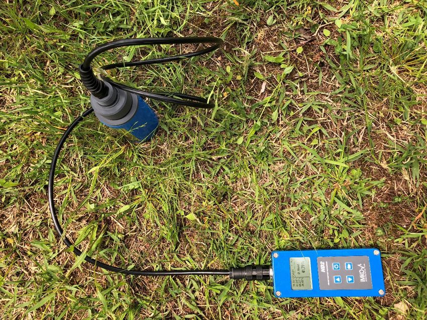
      In order to evaluate the dielectric constant of the soil, the time-domain reflectometry (TDR)
usually required. According to [27,30], the sampling rate ∆x must be equal to or less than the Nyquist
technique was used at several locations in the measurement area, as shown in Figure 2. The average
sampling rate ∆xs along the direction of investigation and cross-investigation for the full-resolution
value of the volumetric water content in the subsurface material was 42%, so that the subsurface
3D imaging:
could be classified as a wet soil. The relative permittivityλmeasured near the soil surface was 27 which
was calculated using the equation described             ∆x ≤in∆x  s =
                                                                [31–33].  The corresponding subsurface velocity was        (1)
                                                                       sinθ
0.06 m/ns.
where    θ is the main lobe angle of the antenna that was used in the investigation and λ is the wavelength
of theAccording
         subsurfacetomaterial.
                           the parameters
                                      Since theofmain the lobe
                                                           500 MHz
                                                                 angle RAMAC
                                                                        of the GPR  shielded
                                                                                      antennaantenna
                                                                                                 used in intheTable   1, the
                                                                                                               near field    is
underground        velocity     ◦  is equal  to  0.06   m/ns,  and   the  spatial sampling    interval
usually greater than 60 , the maximum space interval should be equal to or less than one-quarter        is  equal  to or less
than 5.5 cm.ofTherefore,
wavelength          the antenna  thebandwidth
                                      interval along     thesubsurface
                                                     on the   investigation
                                                                          [27].direction should set less than 5.5 cm to
meetInthe order to evaluate the dielectric constant of the soil,these
              conditions     of  full-resolution      3D  imaging.    Under           circumstances,
                                                                                the time-domain         the system (TDR)
                                                                                                     reflectometry     could
provide    a  3D  subsurface      image   with   5.5   cm  of horizontal   resolution  and 6.7  cm
technique was used at several locations in the measurement area, as shown in Figure 2. The average   of vertical  resolution
in thisofsurvey
value              scenario. water
           the volumetric       Moreover,     it isinworth
                                        content             mentioning
                                                      the subsurface       that an
                                                                       material     excess
                                                                                  was  42%,ofso900
                                                                                                thatmthe
                                                                                                      of surveys
                                                                                                          subsurfacewith  the
                                                                                                                       could
GlobalSat      GPS   Receiver     were   performed      in approximately     half  an hour.  In particular,
be classified as a wet soil. The relative permittivity measured near the soil surface was 27 which            more   than   90
surveys    have   been    carried   out  across   the  4-m  cross  survey   direction. The raw
was calculated using the equation described in [31–33]. The corresponding subsurface velocity wasradargram     of the whole
tree root
0.06 m/ns.survey is shown in Figure 3. A superposition of multiple responses could be seen up to 30
ns.

      Figure 2. Time-domain reflectometry (TDR) measurements of the soil moisture for the estimation of
      Figure 2. Time-domain reflectometry (TDR) measurements of the soil moisture for the estimation of
      the subsurface velocity in the site.
      the subsurface velocity in the site.

      According to the parameters of the 500 MHz RAMAC shielded antenna in Table 1, the underground
velocity v is equal to 0.06 m/ns, and the spatial sampling interval is equal to or less than 5.5 cm. Therefore,
the interval along the investigation direction should set less than 5.5 cm to meet the conditions of
full-resolution 3D imaging. Under these circumstances, the system could provide a 3D subsurface
image with 5.5 cm of horizontal resolution and 6.7 cm of vertical resolution in this survey scenario.
Moreover, it is worth mentioning that an excess of 900 m of surveys with the GlobalSat GPS Receiver
were performed in approximately half an hour. In particular, more than 90 surveys have been carried
out across the 4-m cross survey direction. The raw radargram of the whole tree root survey is shown in
Figure 3. A superposition of multiple responses could be seen up to 30 ns.

4. Data Processing and Methodology
      The processing presented in this study includes four sequential stages. In the pre-processing
stage, time correction and a signal noise filter were applied to increase the clutter rate of the entire
data. Then, by using the local GEONET station, Ultra-Rapid ephemeris, precise clock data, and an
optimisation    algorithm
      Figure 3. Raw       wereofable
                    radargram         to obtain
                                 the tree        accurate location
                                          root investigation          information,
                                                             using a 500 MHz RAMAC which was antenna
                                                                                     shielded used. Next,
the near-field
      system. Kirchhoff migration was used to map the distribution of the coarse roots. In the last stage,
a novel processing scheme was used to identify and clearly map the coarse roots of the investigated
tree. All the algorithms in each stage were implemented in MATLAB.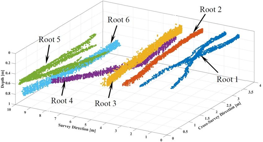
Figure 2. Time-domain reflectometry (TDR) measurements of the soil moisture for the estimation of
Remote Sens. 2020, 12, 1300                                                                           5 of 16
      the subsurface velocity in the site.

      Figure 3. Raw radargram of the tree root investigation using a 500 MHz RAMAC shielded
      Figure 3. Raw radargram of the tree root investigation using a 500 MHz RAMAC shielded antenna
      antenna system.
      system.
4.1. Radargram Signal Processing
     Prior to any interpretation attempt, the raw data were subject to a pre-processing step in
order to reduce undesired reflections and increase the overall signal-to-clutter ratio. In particular,
the pre-processing step consisted of:
(a)   Time-zero adjustment
     This step is applied to adjust the initial position of the surface reflection in GPR signals (the time
when the radar signal spreads out from the antenna and enters the ground is known as “zero time”).
In order to move all traces to the zero-time position before other processing methods, time-zero
adjustment must be applied.
(b)   Background removal
     Cross-coupling between the transmitter and the receiver as well as a ringing noise and multiple
reflections can mask the less dominant reflections from the root. In order to mitigate such unwanted
signals, background removal methods should be applied. Subtracting the background signal proved
very effective for the investigated case study.
(c)   Band-pass filtering
     In order to improve the quality of the data, a band-pass filter is applied to eliminate different types
of noise in this stage. In addition, filters are also used to extract useful information and hidden patterns
from the recorded data. In order to remove the direct current offset and suppress the high-frequency
noise, a band-pass filter was employed with the cut off frequencies FLow and FHigh indicated in Table 1.

4.2. Post-Processing of the Tracking Position
     After pre-processing the GPR raw data, the post-processing will be performed on the GPR
trace position data collected by the low-cost GPS receiver. So that the high precision position of
each GPR trace can be applied for the 3D full resolution imaging for further investigation. GPS
provides continuous global position, time and navigation services. The satellites send navigation and
observation data to the receivers [34–36]. As the GPS receiver is affected by a number of different
parameters, estimating the receiver position is not a trivial task. These parameters include GPS receiver
clock bias, troposphere, ionosphere, multipath propagation and so on [37,38].
     Each of these factors can be modelled separately. The basic pseudo-range equation is given as [39]:

                                 Pm = ρ g + c(∆tr − ∆ts ) + Iε + Tε + εmul ,                              (2)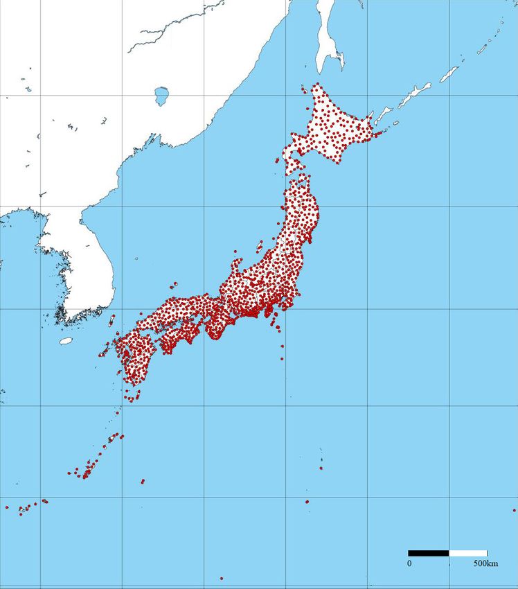
Remote Sens. 2020, 12, 1300                                                                           6 of 16

where c is the speed of light, Tε is the error produced by the troposphere, Iε is the error produced by
the ionosphere and εmul is the multipath error. ∆ts is the offset generated by the satellite bias and ∆tr is
the receiver clock bias. ρ g is the geometric distance from the GPS satellite to the receiver which can be
given by:
                                       q
                                  ρ g = (xr − xs )2 + ( yr − ys )2 + (zr − zs )2 ,                      (3)

where (xr , yr , zr ) and (xs , ys , zs ) are the positional coordinates of the receiver and a given
satellite, respectively.
     In Equation (2), the error term of correction is divided into two groups. The troposphere error,
the ionosphere error and the satellite clock bias are set into one group, represented as Rs . The receiver
clock bias and the multipath error are set into another group, represented as Rr . Therefore, Equation (2)
can be formulated as:
                                    q
                          Pm = (xr − xs )2 + ( yr − ys )2 + (zr − zs )2 + Rs + Rr ,                    (4)

       In Equation (4), the receiver coordinates can be accurately calculated after correctly estimating
the items Rs and Rr . By using signals from at least four satellites at the same time, the GlobalSat
GPS receiver can provide real-time single point positioning [40]. The weakness of GPS comes from
the satellite position, the satellite clock offset and the ionosphere influence, amongst others [41–43].
Nevertheless, the accuracy can be improved by post-processing the received signal.
       Three to nine hours after the observation, the observed Ultra-Rapid ephemeris and clock data can
be obtained online. This information is released four times a day at 03:00, 09:00, 15:00 and 21:00 UTC.
The predicted Ultra-Rapid ephemeris and clock data are also released at the same time, which can be
obtained in advance. Instead, information from Rapid 1 takes longer (from 17 to 41 h) to get online.
It is released every day at 17:00 UTC [44–48].
       International GNSS Service (IGS) is a cooperation with many organisations and countries. This
collects data from more than 300 continuously operating reference stations around the world. Based on
these data, it develops precise satellite ephemeris and clock solutions. The processing phase involves
up to eight IGS analysis centers and the results are freely distributed by IGS. To this effect, this service
allows researchers to post-process the observations based on the information provided by the IGS.
Compared with a broadcast ephemeris and clock correction, the aforementioned approach is more
accurate since these data reflect the precise position and clock offset of the satellite during the actual
measurement. These data are classified into several categories and discussed in the literature [49–51].
       In general, differential processing techniques depend on at least two receivers standing at control
stations (known as a “bases”) with a known location. In Japan, there exist around 1200 GEONET
stations that record data every 30 s, as shown in Figure 4a. Therefore, it is possible to know the
magnitude of the basic position error of the receiver. If the difference between the deviation of the
reference station and the deviation of the flow station can be found, the position error at the reference
line can be calculated. With the differential process, a correction is generated. The procedure can
reduce the position error of unknown points. In general, this method can provide the location with
sub-meter resolution from single-frequency pseudo-range observations. However, this accuracy level
still cannot meet the requirements of current applications.
       It is also worth noting that this application does not require a global solution. Only the 2D relative
position of each GPR acquisition point needs to be estimated accurately. For this purpose, we selected
a reference GEONET station (as shown in Figure 4b) 14 km away from the station. Assuming that the
troposphere error Tε , the ionosphere error Iε and the satellite clock bias of the reference station were the
same as those of the experiment site, the Rs terms in Equation (4) can be directly estimated. Moreover,
the receiver bias ρ g and the multipath error εmul can be estimated and suppressed by designing an
advanced extended Kalman filter.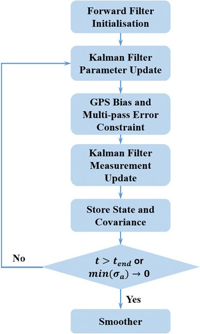
= + ≅ + , (8)
where is the post-processed position of each acquisition point, is the recorded data at each
GPR acquisition point, is the design matrix, which can be replaced by (as described in Figure
5a) and Sens. is
Remote the12,receiver
2020, 1300 clock bias and other minor correction terms such as the multipath error
7 of 16
and the residual error.
(a) (b)
Figure
Figure (a)(a)
4. 4. TheThe location
location of of
thethe GEONET
GEONET stations
stations in in Japan;
Japan; (b)(b) location
location of of
thethe investigation
investigation site
site andand
nearest GEONET Station.
nearest GEONET Station.
In Equation (4), Rs is mainly caused by the substantial errors of the positions of the satellites,
the clock offset, the ionosphere correction etc. Using the record data from the reference station,
a correction matrix was designed with the accuracy of the satellite’s positions, clock offset and
ionosphere information, which can be downloaded afterwards from the International GNSS Service
(IGS) database in order to minimise Rresidual . The measurement equation could be written as:
xre f
Pr = H0 yre f + Rresidual ,
(5)
zre f
where Pr is the post-processed position of the reference station, xre f , yre f , zre f are the recorded
coordinates of the data at the reference station, H0 is the design matrix that contains the satellite and
the reference station receiver clock biases plus the ionospheric and tropospheric effects and another
minor correction term.(a) Lastly, Rresidual is the residual error. (b)
Based
Figure 5. on the aforementioned,
(a) GPS receiver geometry the
withleast squarestation;
a reference term of(b)the residual
flowchart of error Rs receiver
the GPS in the experiment
bias
period can be written as:
estimation and removal by use of the Kalman filter.
RLS = RTresidual Rresidual . (6)
Consequently, the optimally-designed matrix H0 can be calculated as:
min kH0T H0 x − H0T yk2 = 0 (7)
RLS →0
and Equation (4) can be written as:
xr xr
Pm = H yr + Rs H0 yr + Rs , (8)
zr zr
where Pm is the post-processed position of each acquisition point, x is the recorded data at each GPR
acquisition point, H is the design matrix, which can be replaced by H0 (as described in Figure 5a) and
Rs is the receiver clock bias and other minor correction terms such as the multipath error and the
residual error.(a) (b)
Figure
Remote Sens. 4.12,
2020, (a)1300
The location of the GEONET stations in Japan; (b) location of the investigation site and
8 of 16
nearest GEONET Station.
(a) (b)
Figure
Figure 5. 5.(a)(a)GPS
GPSreceiver
receivergeometry
geometrywith witha areference
reference station;(b)(b)
station; flowchartofof
flowchart the
the GPS
GPS receiver
receiver bias
bias
estimation
estimation andand removal
removal byby use
use of of
thethe Kalman
Kalman filter.
filter.
The Rs term is estimated and removed based on the conventional Kalman forward-backward filter.
The estimated offset of the receiver clock located at the tracking station does not represent the actual
offset due to the fact that the obtained observation data were pre-processed [52–54]. An apriority bias
of the GPS receiver was used in the beginning to estimate the term Rs . Finally, all measurements were
then corrected by the terms H and Rs .
In order to update the filter over time, the predictive state vector of the system model should be
used. Since the GPS receiver bias is assumed to be a linear function of time, the drift and all the other
parameters can be considered as constants. It is worth noting that the drift is not strictly the same, as it
will change slowly with time. Figure 5b depicts the complete flowchart of the proposed methodology
consisting of six distinct and sequential steps:
(a) Forward Filter Initialisation
The coarse value of the GlobalSat GPS receiver is used as a prior value for the bias and the drift,
with all the other elements set to zero. In addition, the noise of the filter needs to be set in this step.
(b) GPS Bias and Multi-Pass Error Constraint
In this step, the GPS bias and multi-pass error will propagate towards the current filter state.
(c) Kalman Filter Measurement Update
After the filter run is finished, a state vector computes the mean of the forward and backward
results of the filter state.
(d) Results and Covariance Matrix
In this step, the results are stored to be used in the subsequent filter at this stage. In the meantime,
the covariance matrix is needed to be evaluated. Then, the smoothing factor should be calculated.
(e) Judgement
The procedure is repeated until the processing reaches the end time, or until it meets the constraint
condition. Here, Allen variance σa is used to obtain a rough estimate of the expected receiver bias
and residual error. The Allan variance σa is a measure of frequency stability in clocks, oscillators and
amplifiers [37].
(f) Smooth operatorRemote Sens. 2020, 12, 1300 9 of 16
After all the procedures are finished, the Kalman filter parameters are stored and used to design
the smooth operator.
Figure 6a shows the moving trajectories of the antennas recorded by the GlobalSat GPS receiver.
During the investigation, the effects of the ionosphere had little to negligible effects to the overall
precision of the algorithm. In fact, the drift of the GPS sensor itself was proven to have the biggest
impact on the overall accuracy. The results after applying the Kalman filter and after converting the
data to a local Cartesian coordinate system are shown in Figure 6b. The shape of the trajectory was
consistent with the actual GPR system movement.
Remote Sens. 2020, 01, x FOR PEER REVIEW 9 of 16
(a) (b)
Figure
Figure 6. Moving
6. Moving trajectories
trajectories of antennas
of antennas recorded
recorded by theby the GlobalSat
GlobalSat GPS receiver.
GPS receiver. (a) The (a) The by
record record
the by
the GlobalSat
GlobalSat GPS receiver;
GPS receiver; (b) post-processing
(b) post-processing results. results.
4.3. 4.3.
Kirchhoff Migration
Kirchhoff Migration
In order to detect
In order the the
to detect three-dimensional
three-dimensional distribution
distribution of the treetree
of the roots, a high-resolution
roots, a high-resolution andand
accurate imaging algorithm was implemented in this section. The underground
accurate imaging algorithm was implemented in this section. The underground 3D geometry can 3D geometry can be be
reconstructed
reconstructedfrom the results
from of dense
the results measurements.
of dense measurements. Three-dimensional
Three-dimensional migration is required
migration to to
is required
focus reflection and diffraction and collapse the recorded hyperbolas to their
focus reflection and diffraction and collapse the recorded hyperbolas to their origin [55,56]. origin [55,56].
In this research,
In this weweapplied
research, appliedthe theKirchhoff
Kirchhoff migration,
migration, which which isisbased basedonon thethe generalised
generalised wave-
wave-equation [57,58]. Mathematically, the Kirchhoff migration method can
equation [57,58]. Mathematically, the Kirchhoff migration method can be formulated in the time be formulated in the time
domain as follows:
domain as follows:
1 = ∂R 1 ∂
Z " #
( ) 1+
U(r, t) =U(r, t) U ( r 0 , t −, τ −
) + U ( r0
(, t ,
− τ −
) ) 0. .
dS (9) (9)
8π2 S0 ∂n vR ∂t R2
where represents a source-free surface; is the unit vector normal to ; is the positional
where S0 represents
vector a source-free
of the estimated field; n isisthe
wavesurface; unit
the vectortoofS0the
vector normal
positional ; r isintegration
the positional vector is
point; of the
the estimated wave field; r
propagation speed in media, 0 is the positional vector of the integration
represents the wave field within the surface point; v is the propagation
and speed
in media, U represents the wave field within the surface S0 and
= | − |, (10)
R = |r − r0 |, (10)
= . (11)
R
τ= . (11)
Normally, the far-field approximation /v ≫ 1⁄ is applied in (9). Therefore, the second
term of Equation
Normally, (9) can
the far-field be omitted.ω/Rv
approximation Since
we 2 is applied in (9). Therefore, the second term
1/Rwere oriented in the near-field target, such an
assumption
of Equation wasbe
(9) can noomitted.
longer suitable
Since weforwere
the purpose
oriented ofin this research. To
the near-field mitigate
target, suchthat, the entirety of
an assumption
wasEquation
no longer(9) was used
suitable for in
thethe currentofstudy.
purpose this research. To mitigate that, the entirety of Equation (9)
was usedAs in described
the currentinstudy.
Section 3, TDR measurements were conducted at different points within the
surveying area. The average of the results turned out to provide a wet soil with a volumetric water
content of 42% found using the Topp equation. The measured relative permittivity in the near-surface
of the soil was 27 with a corresponding subsurface velocity of 0.06 m/ns. Since most of the roots were
located in the shallow region of the subsurface, a constant velocity of the medium was assumed in
this paper.Remote Sens. 2020, 12, 1300 10 of 16
As described in Section 3, TDR measurements were conducted at different points within the
surveying area. The average of the results turned out to provide a wet soil with a volumetric water
content of 42% found using the Topp equation. The measured relative permittivity in the near-surface
of the soil was 27 with a corresponding subsurface velocity of 0.06 m/ns. Since most of the roots were
located in the shallow region of the subsurface, a constant velocity of the medium was assumed in
this paper.
5. Results and Discussion
The previous section presented the processing methodology of our proposed strategy for tree root
mapping and assessment. In this section, the results concerning the 3D distribution of the roots system
from
Remotethe
Sens.field
2020,measurements will be discussed.
01, x FOR PEER REVIEW 10 of 16
5.1. 3D Migration
5.1. 3D Migration Result
Result
The
The 3D
3D migration
migration results
results were
were obtained
obtained byby applying the Kirchhoff
applying the Kirchhoff migration discussed above.
migration discussed above.
One-twentieth of the resolution was applied as the grid size during the migration progressing.
One-twentieth of the resolution was applied as the grid size during the migration progressing. Figure Figure 7
shows
7 showsthethemigrated
migratedvertical
verticalprofiles
profilesalong
alongthe
thesurvey
surveydirection
directionatat different
different cross-survey
cross-survey directions
directions
(0.8
(0.8 m, 1.6 m, 2.4 m and 3.2 m). Most of the reflections are located in the upper region from 0.2
m, 1.6 m, 2.4 m and 3.2 m). Most of the reflections are located in the upper region from 0.2 mm to
to
0.5 m. In Figure 7c,d, there is a deep reflection located around 0.7 m depth between the
0.5 m. In Figure 7c,d, there is a deep reflection located around 0.7 m depth between the section 9–10 section 9–10 m
along
m alongthethe
survey
survey direction. Figures
direction. Figure88and
and9Figure
show the migrated
9 show horizontal
the migrated slices atslices
horizontal different depths
at different
(0.16 m, 0.19 m, 0.275 m, 0.42 m, 0.59 m and 0.795 m). By displaying animation frames
depths (0.16 m, 0.19 m, 0.275 m, 0.42 m, 0.59 m and 0.795 m). By displaying animation frames of slices of slices with
different migration
with different depths,
migration the root
depths, thereflections at each
root reflections athorizontal slice are
each horizontal clearly
slice visible.
are clearly visible.
(a) (b)
(c) (d)
7. Migrated
Figure 7. Migratedvertical
verticalprofiles
profiles along
along thethe survey
survey direction.
direction. (a) Migrated
(a) Migrated profile
profile at 0.8 at 0.8 m cross-
m cross-survey
survey direction;
direction; (b) migrated
(b) migrated profile at profile at 1.6 m cross-survey
1.6 m cross-survey direction;
direction; (c) migrated(c) migrated
profile at 2.4profile at 2.4 m
m cross-survey
direction; (d) direction;
cross-survey migrated profile at 3.2 m
(d) migrated cross-survey
profile at 3.2 m direction.
cross-survey direction.Remote Sens. 2020, 12, 1300 11 of 16
Remote Sens. 2020, 01, x FOR PEER REVIEW 11 of 16
(a) (b) (c)
Figure
Figure 8. Migrated
8. Migrated horizontalslices
horizontal slicesatatdifferent
different depths.
depths. Red
Red lines
linesindicate
indicatethe
thedetected
detectedroots inin
roots thethe
migrated data set. (a) Migrated slice at 16-cm depth; (b) migrated slice at 19-cm depth; (c)
migrated data set. (a) Migrated slice at 16-cm depth; (b) migrated slice at 19-cm depth; (c) migrated migrated
slice
slice at 27.5-cm
at 27.5-cm depth.
depth.
(a) (b) (c)
Figure 9. Migrated horizontal slices at different depths. Red lines indicate the detected roots in the
migrated data set. (a) Migrated slice at 42-cm depth; (b) migrated slice at 59-cm depth; (c) migrated
slice at 79.5-cm depth.Based on the migration results, it was also obvious that most of the reflections from the roots
were located in the upper region, as shown in Figure 8. In the figures, some areas with a strong
amplitude showed the bright blocks feature. These bright blocks appear to be randomly distributed,
and they
Remote can be
Sens. 2020, 12, mainly
1300 attributed to the heterogeneity of the soils, rocks and similar features12inofthe 16
subsurface. Hence, it is difficult to discriminate coarse roots by using GPR from these output types.
There are many reasons that limits the applicability and the accuracy of GPR for detecting tree
Based on the migration results, it was also obvious that most of the reflections from the roots were
roots. For example, if a cluster of fine roots surrounds a deeper coarse root, it is difficult to detect the
located in the upper region, as shown in Figure 8. In the figures, some areas with a strong amplitude
coarse root. Moreover, if the distance between two coarse roots is less than the horizontal and vertical
showed the bright blocks feature. These bright blocks appear to be randomly distributed, and they
resolution of the observation system at the same time, then two coarse roots will be considered as a
can be mainly attributed to the heterogeneity of the soils, rocks and similar features in the subsurface.
unique root. In addition, roots that are parallel to the polarisation of the antenna will result in weak
Hence, it is that
reflections difficult
willtobediscriminate coarse roots
masked by unwanted by using
clutter and GPR
noise.from
Basedthese output
on the types.
aforementioned factors,
There
the root canarebemany
detectedreasons that limits
according to thethe applicability
reflection anddirection
intensity, the accuracy of GPR for detecting
and surrounding tree
environment
roots. For example, if a cluster of fine roots surrounds a deeper coarse root,
from the migrated slices. The distribution of tree roots must be mapped on a three-dimensionalit is difficult to detect the
coarse root. Moreover,
environment, if the distance
as the reflection between
amplitude twosame
in the coarse rootsslice
depth is less thanalong
varies the horizontal
the root. and verticala
Therefore,
resolution of the observation system at the same time, then two coarse roots will be
coherent 3D approach is necessary in order to effectively locate and track the distribution of the roots. considered as a
unique root. In addition, roots that are parallel to the polarisation of the antenna will result in weak
reflections
5.2. 3D RootsthatDetection
will be masked
Result by unwanted clutter and noise. Based on the aforementioned factors,
the root can be detected according to the reflection intensity, direction and surrounding environment
from The root distribution
the migrated can be
slices. The tracked from
distribution the image
of tree index.
roots must beThe coarseon
mapped tree roots normally can
a three-dimensional
be displayed continuously
environment, as the reflectionin the 3D migrated
amplitude data.
in the sameTherefore, these
depth slice image
varies indexes
along the can beTherefore,
root. associated
a coherent 3D approach is necessary in order to effectively locate and track the distribution ofwere
with the root. In this paper, high-energy regions inside a 3D cube above a certain threshold used
the roots.
to extract root locations. In Figure 10a, a B-scan profile which contains a tree root is shown. The profile
is perpendicular
5.2. 3D Roots Detectionto theResult
root extension direction. In this migrated cube, a 1.5 m × 1.5 m × 0.3 m (survey
direction × cross-survey direction × depth) block was selected. The peak position of the cube was
The root distribution can be tracked from the image index. The coarse tree roots normally can be
found and a vertical curve (depth) and two horizontal curves (survey and cross-survey directions) of
displayed continuously in the 3D migrated data. Therefore, these image indexes can be associated
the peak were used for next step analysis. Additionally, the −3 dB width of the peak is defined as the
with the root. In this paper, high-energy regions inside a 3D cube above a certain threshold were used
root in each direction, as it is shown in Figure 10b,c.
to extract root locations. In Figure 10a, a B-scan profile which contains a tree root is shown. The profile
Overall, the accuracy of the root detection using pixel intensities in the image was slightly worse
is perpendicular to the root extension direction. In this migrated cube, a 1.5 m × 1.5 m × 0.3 m (survey
than extracting the feature directly from the waveform. The –3-dB threshold did not remove all the
direction × cross-survey direction × depth) block was selected. The peak position of the cube was
weak reflections, such as those from the heterogeneous soils, rocks, and fine roots. To avoid false
found and a vertical curve (depth) and two horizontal curves (survey and cross-survey directions) of
detection results, future processing should also include discarding those targets that do not have
the peak were used for next step analysis. Additionally, the −3 dB width of the peak is defined as the
continuous distribution.
root in each direction, as it is shown in Figure 10b,c.
(a) (b) (c)
Figure10.
Figure 10.The
Thecoarse
coarseroot
rootdetection
detectionin
inaa3D
3Dmigrated
migratedcubic:
cubic: (a)
(a)B-scan
B-scanprofile
profilewhich
whichcontains
containsaatree
tree
root.(b)
root. (b)Root
Rootextension
extensiontracking
trackingwith
withthe
the−3
−3 dB
dB positions
positionsof
ofaalocal
localpeak
peak(survey
(surveydirection).
direction).(c)
(c)Root
Root
extensiontracking
extension trackingwith
withthe
the−3
−3 dB
dB positions
positions of
of aalocal
localpeak
peak(cross-survey
(cross-surveydirection).
direction).
Overall, the accuracy of the root detection using pixel intensities in the image was slightly worse
than extracting the feature directly from the waveform. The –3-dB threshold did not remove all the
weak reflections, such as those from the heterogeneous soils, rocks, and fine roots. To avoid false
detection results, future processing should also include discarding those targets that do not have
continuous distribution.
The reconstructed 3D root system is illustrated from two different viewpoints in Figure 11.
Six coarse roots across the survey direction can be clearly detected. The false detection results were
discarded. Root 1, 2, 3 and 4 were located at the 30-cm region below the subsurface and theirRemote Sens. 2020, 01, x FOR PEER REVIEW 13 of 16
RemoteThe
Sens.reconstructed
2020, 12, 1300 3D root system is illustrated from two different viewpoints in Figure 11. 13 ofSix
16
coarse roots across the survey direction can be clearly detected. The false detection results were
discarded. Root 1, 2, 3 and 4 were located at the 30-cm region below the subsurface and their
distributions
distributions were
were confirmed
confirmed with
with aa thin
thin measuring
measuring flower
flower pole,
pole, which
which can
can bebe inserted
inserted into
into the
the soil
soil
and record the depth of these targets. Root 5 and 6 were located at 0.5 m and 0.7 m,
and record the depth of these targets. Root 5 and 6 were located at 0.5 m and 0.7 m, respectively. respectively. In the
In
field data data
the field set, itset,
wasitimpossible to detect
was impossible to all the coarse
detect all theroots.
coarseThe characteristics
roots. of tree roots
The characteristics radiating
of tree roots
along the along
radiating trunk the
provided an assumption
trunk provided for identifying
an assumption the extension
for identifying of the roots.
the extension Onroots.
of the the contrary,
On the
fine roots always gather on heterogeneous soil and stone. This is because it is not
contrary, fine roots always gather on heterogeneous soil and stone. This is because it is not conduciveconducive to the
growth of trachyte
to the growth in theseinareas.
of trachyte theseSince
areas.there
Sincewas no was
there marked difference
no marked betweenbetween
difference the fine the
roots and
fine the
roots
surrounding environment, it was difficult to find these targets.
and the surrounding environment, it was difficult to find these targets.
(a)
(b)
Figure 11.
Figure 11. The reconstructed 3D root system: (a)
(a) View from the starting point; (b) view from the
the
ending point.
ending point.
6. Conclusions
6. Conclusions
In
In this
this paper,
paper, aa low-cost
low-cost GPS
GPS receiver
receiver combined
combined with with aa 500
500 MHz
MHz RAMAC
RAMAC shielded
shielded antenna
antenna was
was
used
used to toobtain
obtainaafull-resolution
full-resolution3D 3Dimage
image ofof
thethe
root system
root of several
system larch
of several trees.
larch By using
trees. By usingthe low-cost
the low-
GPS receiver
cost GPS and advanced
receiver and advancedprocessing algorithms,
processing algorithms,an effective and affordable
an effective and affordableway way
for mapping tree
for mapping
root systems was proposed. This equipment combination was used to carry
tree root systems was proposed. This equipment combination was used to carry out a full-resolution out a full-resolution
survey over aa 10
survey over m××44mmarea
10 m areaininapproximately
approximately half
half anan hour,
hour, which
which proved
proved thethe
timetime efficiency
efficiency of
of the
the
approach proposed. In addition, a dedicated post-processing methodology was implemented to
approach proposed. In addition, a dedicated post-processing methodology was implemented to
enhance
enhance the the accuracy
accuracy of of each
each GPR
GPR trace
trace recorded
recorded by by the
the low-cost
low-cost GPS
GPS receiver.
receiver. After that, aa Kirchhoff
After that, Kirchhoff
migration
migration approach
approach considering
considering the the near
near field
field effects
effects was
was applied
applied toto accurately
accurately mapmap thethe investigated
investigated
root system. Lastly, the 3D distribution of coarse roots was mapped
root system. Lastly, the 3D distribution of coarse roots was mapped by considering by considering the local magnitude
the local
in a 3D migrated
magnitude in a 3D cube. As a cube.
migrated result,As sixalarge
result,coarse rootscoarse
six large were roots
successfully identified. identified.
were successfully Although
it is not possible
Although it is not to have full
possible detection
to have of the entire
full detection of theroot system
entire (i.e., coarse
root system and fine
(i.e., coarse and roots), this
fine roots),Remote Sens. 2020, 12, 1300 14 of 16
research demonstrates the potential of combining low-cost GPS and GPR antenna systems to achieve a
full-resolution 3D GPR survey in a time-effective and affordable manner.
Author Contributions: L.Z. analysed the data, proposed the algorithm and wrote the paper. Y.W. contributed
to data analysis and provided useful suggestions. I.G., F.T. and A.M.A. contributed in structuring the focus of
the paper and the presentation of the results, as well as in editing the language. M.S. contributed much to the
experimental design, data collection, and language correction. All authors have read and agreed to the published
version of the manuscript.
Funding: This research received no external funding.
Conflicts of Interest: The authors declare no conflict of interest.
References
1. Stokes, A.; Fitter, A.H.; Courts, M.P. Responses of young trees to wind and shading: Effects on root
architecture. J. Exp. Bot. 1995, 46, 1139–1146. [CrossRef]
2. Coutts, M.P. Root architecture and tree stability. Plant Soil 1983, 71, 171–188. [CrossRef]
3. Habermehl, A. A new non-destructive method for determining internal wood condition and decay in living
trees. Part 1. Principles, method, and apparatus. Arboric. J. 1982, 6, 1–8. [CrossRef]
4. Habermehl, A. A new non-destructive method for determining internal wood condition and decay in living
trees. II: Results and further developments. Arboric. J. 1982, 6, 121–130. [CrossRef]
5. Daniels, D.J. Ground Penetrating Radar, 2nd ed.; Institution of Engineering and Technology: London, UK, 2004.
6. Harry, M.J. Ground Penetrating Radar: Theory and Application, 1st ed.; Elsevier Science: Amsterdam,
The Netherlands, 2009.
7. Vore, S.L.D. Ground-penetrating radar: An introduction for archaeologists. Geoarchaeology 1997, 54, 527–528.
[CrossRef]
8. Kaur, P.; Dana, K.J.; Romero, F.A.; Gucunski, N. Automated GPR rebar analysis for robotic bridge deck
evaluation. IEEE Control Syst. Lett. 2015, 46, 2265–2276. [CrossRef]
9. Zou, L.; Yi, L.; Sato, M. On the Use of Lateral Wave for the Interlayer Debonding Detecting in an Asphalt
Airport Pavement Using a Multistatic GPR System. IEEE Trans. Geosci. Remote Sens. 2020, 58, 1–10,
(early access). [CrossRef]
10. Zhou, H.; Sato, M. Archaeological investigation in Sendai Castle using ground-penetrating radar.
Archaeol. Prospect. 2001, 8, 1–11. [CrossRef]
11. Sato, M.; Hamada, Y.; Feng, X.; Kong, F.N.; Zeng, Z.; Fang, G. GPR using an array antenna for landmine
detection. Near Surf. Geophys. 2004, 2, 7–13. [CrossRef]
12. Slob, E.; Sato, M.; Olhoeft, G. Surface and borehole ground-penetrating-radar developments. Geophysics
2010, 75, 75A103–75A120. [CrossRef]
13. Hruska, J.; Čermák, J.; Šustek, S. Mapping tree root systems with ground-penetrating radar. Tree Physiol.
1999, 19, 125–130. [CrossRef] [PubMed]
14. Butnor, J.R.; Doolittle, J.A.; Kress, L.; Cohen, S.; Johnsen, K.H. Use of ground-penetrating radar to study tree
roots in the southeastern United States. Tree Physiol. 2001, 21, 1269–1278. [CrossRef] [PubMed]
15. Barton, C.V.; Montagu, K.D. Detection of tree roots and determination of root diameters by ground penetrating
radar under optimal conditions. Tree Physiol. 2004, 24, 1323–1331. [CrossRef] [PubMed]
16. Butnor, J.R.; Doolittle, J.A.; Johnsen, K.H.; Samuelson, L.; Stokes, T.; Kress, L. Utility of ground-penetrating
radar as a root biomass survey tool in forest systems. J. Soil Sci. 2003, 67, 1607–1615. [CrossRef]
17. Hirano, Y.; Dannoura, M.; Aono, K.; Igarashi, T.; Ishii, M.; Yamase, K.; Makita, N.; Kanazawa, Y. Limiting
factors in the detection of tree roots using ground-penetrating radar. Plant Soil. 2009, 319, 15. [CrossRef]
18. Zenone, T.; Morelli, G.; Teobaldelli, M.; Fischanger, F.; Matteucci, M.; Sordini, M.; Armani, A.; Ferrè, C.;
Chiti, T.; Seufert, G. Preliminary use of ground-penetrating radar and electrical resistivity tomography to
study tree roots in pine forests and poplar plantations. Plant Physiol. 2008, 35, 1047–1058. [CrossRef]
19. Liu, H.; Huang, X.Y.; Han, F.; Cui, J.; Spencer, B.F.; Xie, X.Y. Hybrid Polarimetric GPR Calibration and
Elongated Object Orientation Estimation. IEEE J. Sel. Top. Appl. Earth. Obs. Remote Sens. 2019, 12, 2080–2087.
[CrossRef]Remote Sens. 2020, 12, 1300 15 of 16
20. Cui, X.; Guo, L.; Chen, J.; Chen, X.; Zhu, X. Estimating tree-root biomass in different depths using
ground-penetrating radar: Evidence from a controlled experiment. IEEE Trans. Geosci. Remote Sens. 2012,
51, 3410–3423. [CrossRef]
21. Raz-Yaseef, N.; Koteen, L.; Baldocchi, D.D. Coarse root distribution of a semi-arid oak savanna estimated
with ground penetrating radar. J. Geophys. Res. Earth Surf. 2013, 118, 135–147. [CrossRef]
22. Li, W.; Cui, X.; Guo, L.; Chen, J.; Chen, X.; Cao, X. Tree Root Automatic Recognition in Ground Penetrating
Radar Profiles Based on Randomized Hough Transform. Remote Sens. 2016, 8, 430. [CrossRef]
23. Leucci, G. The use of three geophysical methods for 3D images of total root volume of soil in urban
environments. Explor. Geophys. 2010, 41, 268–278. [CrossRef]
24. Tanikawa, T.; Hirano, Y.; Dannoura, M.; Yamase, K.; Aono, K.; Ishii, M.; Igarashi, T.; Ikeno, H.; Kanazawa, Y.
Root orientation can affect detection accuracy of ground-penetrating radar. Plant Soil. 2013, 373, 317–327.
[CrossRef]
25. Alani, A.M.; Lantini, L. Recent advances in tree root mapping and assessment using non-destructive testing
methods: A focus on ground penetrating radar. Surv. Geophys. 2020, 41, 605–646. [CrossRef]
26. Tosti, F.; Bianchini Ciampoli, L.; Brancadoro, M.G.; Alani, A. GPR applications in mapping the subsurface
root system of street trees with road safety-critical implications. Adv. Trans. Stud. 2018, 44, 107–118.
27. Zhu, S.; Huang, C.; Su, Y.; Sato, M. 3D Ground Penetrating Radar to Detect Tree Roots and Estimate Root
Biomass in the Field. Remote Sens. 2014, 6, 5754–5773. [CrossRef]
28. Grasmueck, M.; Viggiano, D.A. Integration of ground-penetrating radar and laser position sensors for
real-time 3-D data fusion. IEEE Trans. Geosci. Remote Sens. 2007, 45, 130–137. [CrossRef]
29. Böniger, U.; Tronicke, J. On the potential of kinematic GPR surveying using a self-tracking total station:
Evaluating system crosstalk and latency. IEEE Trans. Geosci. Remote Sens. 2010, 48, 3792–3798. [CrossRef]
30. Rial, F.I.; Pereira, M.; Lorenzo, H.; Arias, P.; Novo, A. Resolution of GPR bowtie antennas: An experimental
approach. J. Appl. Geophys. 2009, 67, 367–373. [CrossRef]
31. Böniger, U.; Tronicke, J. Improving the interpretability of 3D GPR data using target-specific attributes:
Application to tomb detection. J. Archaeol. Sci. 2010, 37, 672–679. [CrossRef]
32. Bano, M. Modelling of GPR waves for lossy media obeying a complex power law of frequency for dielectric
permittivity. Geophys. Prospect. 2004, 52, 11–26. [CrossRef]
33. Hanafy, S.; Al Hagrey, S.A. Ground-penetrating radar tomography for soil-moisture heterogeneity. Geophysics
2005, 71, K9–K18. [CrossRef]
34. Misra, P.; Enge, P. Special issue on global positioning system. Proc. IEEE. 1999, 87, 3–15. [CrossRef]
35. Dow, J.M.; Neilan, R.E.; Rizos, C. The international GNSS service in a changing landscape of global navigation
satellite systems. J. Geod. 2009, 83, 191–198. [CrossRef]
36. Groves, P.D. Principles of GNSS, Inertial, and Multisensor Integrated Navigation Systems; Artech House: Norwood,
MA, USA, 2013.
37. Hofmann-Wellenhof, B.; Lichtenegger, H.; Wasle, E. GNSS–Global Navigation Satellite Systems: GPS, GLONASS,
Galileo, and More; Springer Science & Business Media: Berlin, Germany, 2007.
38. Jin, S.; Feng, G.P.; Gleason, S. Remote sensing using GNSS signals: Current status and future directions.
Adv. Space Res. 2011, 47, 1645–1653. [CrossRef]
39. Hegarty, C.J.; Chatre, E. Evolution of the global navigation satellitesystem (gnss). Proc. IEEE 2008,
96, 1902–1917. [CrossRef]
40. Teunissen, P.J. Integer least-squares theory for the GNSS compass. J. Geod. 2010, 84, 433–447. [CrossRef]
41. Montenbruck, O.; Hauschild, A.; Steigenberger, P. Differential code bias estimation using multi-GNSS
observations and global ionosphere maps. Navig. J. Inst. Navig. 2014, 61, 191–201. [CrossRef]
42. Hoque, M.M.; Jakowski, N. Higher order ionospheric effects in precise GNSS positioning. J. Geod. 2007,
81, 259–268. [CrossRef]
43. Jin, R.; Jin, S.; Feng, G. M_DCB: Matlab code for estimating GNSS satellite and receiver differential code
biases. GPS Solut. 2012, 16, 541–548. [CrossRef]
44. Closas, P.; Fernández-Prades, C.; Fernández-Rubio, J.A. Maximum likelihood estimation of position in GNSS.
IEEE Signal Process. Lett. 2007, 14, 359–362. [CrossRef]
45. Wang, N.; Yuan, Y.; Li, Z.; Montenbruck, O.; Tan, B. Determination of differential code biases with multi-GNSS
observations. J. Geod. 2016, 90, 209–228. [CrossRef]You can also read


