Generalized Pythagoras Trees: A Fractal Approach to Hierarchy Visualization
←
→
Page content transcription
If your browser does not render page correctly, please read the page content below
Generalized Pythagoras Trees: A Fractal
                                   Approach to Hierarchy Visualization

                              Fabian Beck1 , Michael Burch1 , Tanja Munz1 , Lorenzo Di Silvestro2 , and
                                                        Daniel Weiskopf1
                                          1
                                            VISUS, University of Stuttgart, Stuttgart, Germany
                          2
                              Dipartimento di Matematica e Informatica, Università di Catania, Catania, Italy

                                  Abstract. Through their recursive definition, many fractals have an in-
                                  herent hierarchical structure. An example are binary branching Pythago-
                                  ras Trees. By stopping the recursion in certain branches, a binary hier-
                                  archy can be encoded and visualized. But this binary encoding is an
                                  obstacle for representing general hierarchical data such as file systems or
                                  phylogenetic trees, which usually branch into more than two subhierar-
                                  chies. We hence extend Pythagoras Trees to arbitrarily branching trees
                                  by adapting the geometry of the original fractal approach. Each vertex
                                  in the hierarchy is visualized as a rectangle sized according to a metric.
                                  We analyze several visual parameters such as length, width, order, and
                                  color of the nodes against the use of different metrics. Interactions help
                                  to zoom, browse, and filter the hierarchy. The usefulness of our technique
                                  is illustrated by two case studies visualizing directory structures and a
                                  large phylogenetic tree. We compare our approach with existing tree di-
                                  agrams and discuss questions of geometry, perception, readability, and
                                  aesthetics.

                                  Keywords: Hierarchy visualization, fractals.

                      1         Introduction

                      Hierarchical data (i.e., trees) occurs in many application domains, for instance,
                      as results of a hierarchical clustering algorithm, as files organized in directory
                      structures, or as species classified in a phylogenetic tree. Providing an overview
                      of possibly large and deeply nested tree structures is one of the challenges in
                      information visualization. An appropriate visualization technique should pro-
                      duce compact, readable, and comprehensive diagrams, which ideally also look
                      aesthetically appealing and natural to the human eye.
                          A prominent visualization method are node-link diagrams, which are often
                      simply denoted as tree diagrams; layout and aesthetic criteria have been dis-
                      cussed [24, 31]. Although node-link diagrams are intuitive and easy to draw, vi-
                      sual scalability and labeling often is an issue. An alternative, in particular easing
                      the labeling problem, are indented trees [7] depicting the hierarchical structure
                      by indentation. Further, layered icicle plots [17] stack boxes on top of each other
                      for encoding a hierarchy, but waste space by assigning large areas to inner nodes

Appeared in: "Computer Vision, Imaging and Computer Graphics Theory and Applications 2014 - Revised Selected Papers"

The final publication is available at link.springer.com.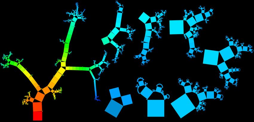
2       Beck, Burch, Munz, Di Silvestro, and Weiskopf

               (a)                         (b)                         (c)

Fig. 1. Extending Pythagoras Trees for encoding information hierarchies: (a) tradi-
tional fractal approach; (b) Generalized Pythagoras Tree applied to an n-ary informa-
tion hierarchy; (c) additionally visualizing the number of leaves by the size of the inner
nodes.

on higher levels of the hierarchy. The Treemap approach [27], which is applying
the concept of nested boxes, produces space-efficient diagrams but complicates
interpreting the hierarchical structure.
     In this paper, we introduce Generalized Pythagoras Trees as an alternative
to the above hierarchy visualization techniques. It is based on Pythagoras Trees
[5], a fractal technique showing a binary hierarchy as branching squares (Fig. 1,
a); the fractal approach is named after Pythagoras because every branch creates
a right triangle and the Pythagorean theorem is applicable to the areas of the
squares. We extend this approach to n-arily branching structures and use it for
depicting information hierarchies (Fig. 1, b). Instead of triangles, each recur-
sive rendering step produces a convex polygonal shape where the corners are
placed on a semi circle. The size of the created rectangles can be modified for
encoding numeric information such as the number of leaf nodes of the respective
subhierarchy (Fig. 1, c).
     We implemented the approach as an interactive tool and demonstrate its
usefulness by applying it to large and deeply structured abstract hierarchy data
from two application domains: a file system organized in directories and the
NCBI taxonomy, a phylogentic tree that structures the living organisms on earth
in a tree consisting of more than 300,000 vertices. Furthermore, a comparison
to existing hierarchy visualization approaches provides first insights into the
unique characteristic of Generalized Pythagoras Trees: a higher visual variety
leads to more distinguishable visualizations, the fractal origin of the method
supports identifying self-similar structures, and the specific layout seems to be
particularly suitable for visualizing deep hierarchies. Finally, the created images
are visually appealing as they show analogies to natural tree and branching
structures.

2    Related Work

The visualization of hierarchical data is a central information visualization prob-
lem that has been studied for many years. Typical respresentations include node-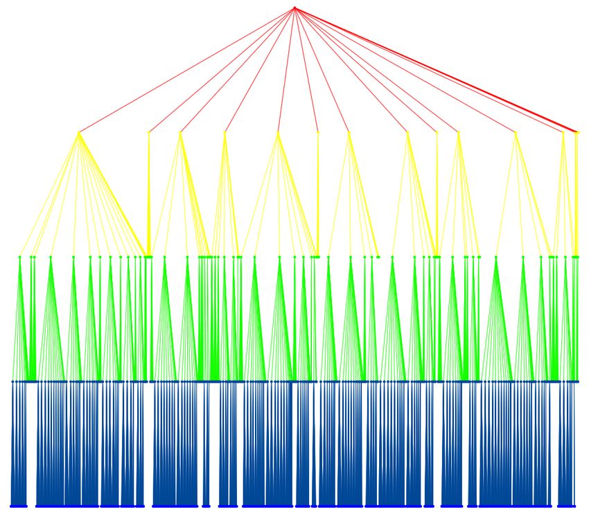
Generalized Pythagoras Trees         3

link, stacking, nesting, indentation, or fractal concepts as surveyed by [13, 26].
Many variants of the general concepts exist, for instance, radial [3, 10] and bubble
layouts [11, 18] of node-link diagrams, circular approaches for stacking techniques
[1, 28, 33], or nested visualizations based on Voronoi diagrams [2, 22].
     Although many tree visualizations were proposed in the past, none provides
a generally applicable solution and solves all related issues. For example, node-
link diagrams clearly show the hierarchical structure by using explicit links in
a crossing-free layout. However, by showing the node-link diagram in the tradi-
tional fashion with the root vertex on top and leaves at the bottom, much screen
space stays unused at the top while leaves densely agglomerate at the bottom.
Transforming the layout into a radial one distributes the nodes more evenly,
but makes comparisons of subtrees more difficult. Node-link layouts of hierar-
chies have been studied in greater detail, for instance, [6] investigated visual task
solution strategies whereas [21] analyzed space-efficiency.
     Indented representations of hierarchies are well-known from explorable lists
of files in file browsers. Recently, [7] investigated a variant as a technique for rep-
resenting large hierarchies as an overview representation. Such a diagram scales
to very large and deep hierarchies and still shows the hierarchical organization
but not as clear as in node-link diagrams. Layered icicle plots [17], in contrast,
use the concept of stacking: the root vertex is placed on top and, analogous to
node-link diagrams, consumes much horizontal space that is as large as all child
nodes together.
     Treemaps [27], a space-filling approach, are a prominent representative of
nesting techniques for encoding hierarchies. While properties of leaf nodes can
be easily observed, a limitation becomes apparent when one tries to explore the
hierarchical structure because it is difficult to retrieve the exact hierarchical in-
formation from deeply nested boxes: representatives of inner vertices are (nearly)
completely covered by descendants. Treemaps have been extended to other lay-
out techniques such as Voronoi diagrams [2, 22] producing aesthetic diagrams
that, however, suffer from high runtime complexity.
     Also, 3D approaches have been investigated, for instance, in Cone Trees [8],
each hierarchy vertex is visually encoded as a cone with the apex placed on the
circle circumference of the parent. Occlusion problems occur that are solved by
interactive features such as rotation. Botanical Trees [14], a further 3D approach,
imitate the aesthetics of natural trees but are restricted to binary hierarchies,
that is, n-ary hierarchies are modeled as binary trees by the strand model of
[12]; it becomes harder to detect the parent of a node.
     The term fractal was coined by [20] and the class of those approaches has also
been used for hierarchy visualization due to their self-similarity property [15, 16].
With OneZoom [25], the authors propose a fractal-based technique for visualizing
phylogenetic trees; however, n-ary branches need to be visually translated into
binary splits. [9] visualize random binary hierarchies with a fractal approach as
botanical trees; no additional metric value for the vertices is taken into account;
instead, they investigate the Horton-Strahler number for computing the branch
thicknesses.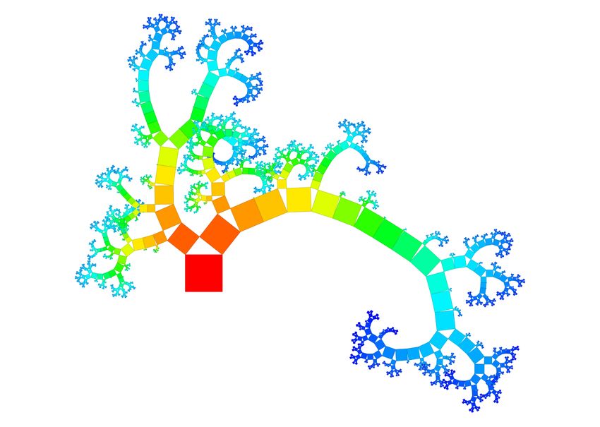
4       Beck, Burch, Munz, Di Silvestro, and Weiskopf

    The goal of our work is to extend a fractal approach, which is closer to
natural tree structures, towards information visualization. This goal promises
embedding the idea of self-similarity and aesthetics of fractals into hierarchy
visualization. Central prerequisite—and in this, our approach differs from exist-
ing fractal approaches—is that n-ary branches should be possible. With respect
to information visualization, the approach targets at combining advantages of
several existing techniques: a readable and scalable representation, an efficient
use of screen space, and the flexibility for encoding additional information. A
downside of the approach, however, is that overlap may occur similar as in 3D
techniques (though it is a 2D representation)—only varying the parameters of
the visualization or using interaction alleviates this issue.

3     Visualization Technique
Our general hierarchy visualization approach extends the idea of Pythagoras
Trees. Instead of basing the branching of subtrees on right triangles, we exploit
convex polygons with edges on the circumference of a semi circle.

3.1   Data Model
We model a hierarchy as a directed graph H = (V, E) where V = {v1 , . . . , vk }
denotes the finite set of k vertices and E ⊂ V × V the finite set of edges, i.e.,
parent–child relationships. One vertex is the designated root vertex and is the
only vertex without an incoming edge; all other vertices have an in-degree of
one. We allow arbitrary hierarchies, that is, the out-degree of the vertices is not
restricted. A maximum branching factor n ∈ N of H can be computed as the
maximum out-degree of all v ∈ V . For an arbitrary vertex v ∈ V , Hv denotes the
subhierarchy having v as root vertex; | Hv | is the number of vertices included
in the Hv (including v). The depth of a vertex v 0 in Hv is the number of vertices
on the path through the hierarchy from v to v 0 . We allow positive weights to be
attached to each vertex of the hierarchy v ∈ V representing metric values such
as sizes. We model them as a function w : V → R. The weight w(v) ∈ R+ of an
inner vertex v does not necessarily need to be the sum of its children, but can
be.

3.2   Traditional Pythagoras Tree
The Pythagoras Tree is a fractal approach describing a recursive procedure of
drawing squares. In that, it was initially not intended to encode information,
but its tree structure easily allows representing binary hierarchies: each square
represents a vertex of the hierarchy; the recursive generation follows the structure
of the hierarchy and ends at the leaves.
    Drawing a fractal Pythagoras Tree starts with drawing a square of side length
c. Then, two smaller squares are attached at one side of the square—usually, at
the top—according to the procedure illustrated in Fig. 2 (a): Then, a right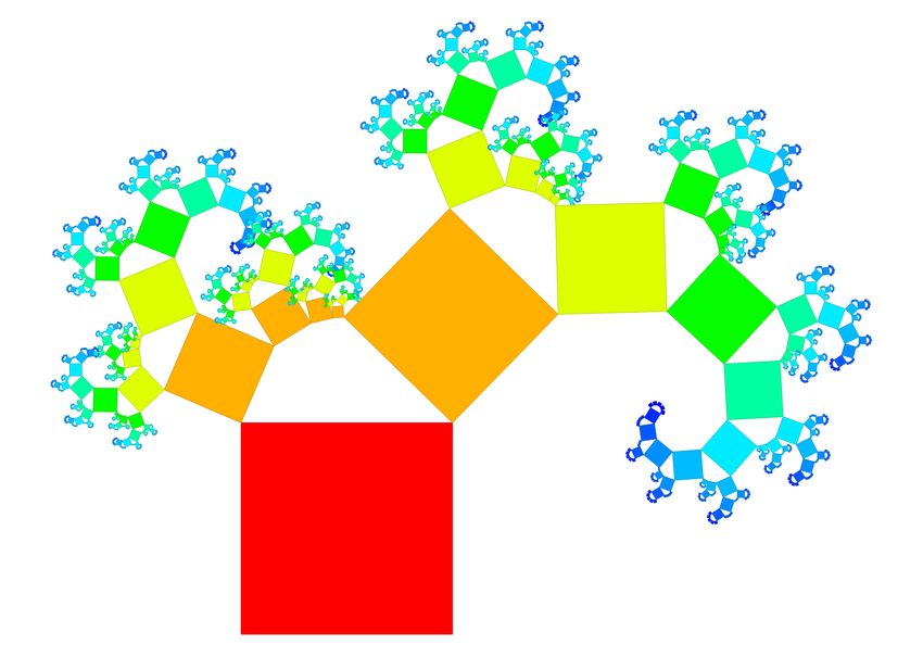
Generalized Pythagoras Trees         5

                 (a)                                     (b)

Fig. 2. Illustration of the traditional Pythagoras Tree approach: (a) a single binary
branch; (b) recursively applied branching step.

triangle with angles α and β where α + β = π2 is drawn using the side of the
square as hypotenuse, which also becomes a diameter of the circumcircle of
the triangle. The two legs of the triangle are completed to squares having side
lengths a and b. In the right triangle, the Pythagorean theorem a2 + b2 = c2
holds, i.e., the sum of the areas of the squares over the legs is equal to the area of
the square over the hypotenuse. Applying this procedure recursively to the new
squares as depicted for the next step in Fig. 2 (b) creates a fractal Pythagoras
Tree (the recursion is only stopped for practical reasons at some depth). The
angles α and β can be set to a constant value or be varied according to some
procedural pattern. Fig. 1 (a) provides an example of a fractal Pythagoras Tree
where α = β = π4 .
    Transforming the fractal approach into an information visualization tech-
nique, the squares are interpreted as representatives of vertices of the hierarchy,
called nodes. As a consequence, the fractal encodes a complete binary hierarchy,
the recursion depth being the depth of the hierarchy. If the generated image
should represent a binary hierarchy that is not completely filled to a certain
depth, the recursion has to stop earlier for the respective subtrees. If the hier-
archy is weighted as specified in the data model, the weights can be visually
encoded by adjusting the sizes of the squares, i.e., the corresponding angles α
and β.
    Algorithm 1 describes in greater detail how an arbitrary binary hierarchy
(i.e., a hierarchy where each vertex either has an out-degree of 2 or 0) can
be recursively transformed into a Pythagoras Tree visualization. It is initiated
by calling PythagorasTree(Hv , S): where Hv = (V, E) is a binary hierarchy
and S = (c, ∆s, θ) is the initial square with center c, length of the sides ∆s,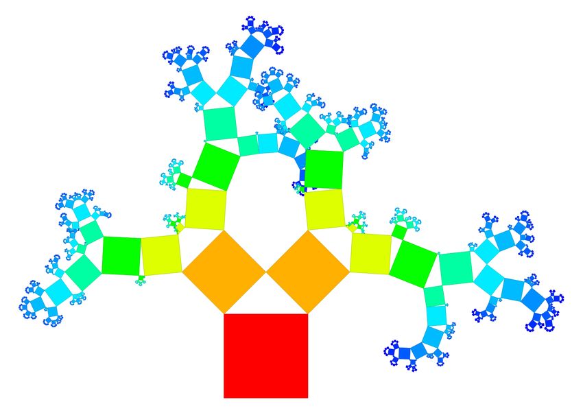
6         Beck, Burch, Munz, Di Silvestro, and Weiskopf

Algorithm 1 Pythagoras Tree
PythagorasTree(Hv , S):
 // Hv : binary hierarchy
    // S: representative square S = (c, ∆s, θ)
      // c = (xc , yc ): center
      // ∆s: length of a side
      // θ: slope angle
    drawSquare(S);     // draw square for current root vertex
    if | Hv |> 1 then
       // v1 and v2 : children of Hv
       α := π2 · w(v1w(v 2)
                      )+w(v2 )
                               ;
      β := π2 · w(v1w(v 1)
                     )+w(v2 )
                              ;
      ∆s1 := ∆s · sin β;
      ∆s2 := ∆s · sin α;
      c1 := ComputeCenterLef t(c, ∆s, ∆s1 , );
      c2 := ComputeCenterRight(c, ∆s, ∆s2 );
      S1 := (c1 , ∆s1 , θ + α);
      S2 := (c2 , ∆s2 , θ − β);
      PythagorasTree(Hv1 , S1 );       // draw subhierarchy Hv1
      PythagorasTree(Hv2 , S2 );       // draw subhierarchy Hv2
    end if

and slope angle θ. The recursive procedure first draws square S and proceeds
if the current hierarchy still contains more than a single node. Then, encoding
the node weights in the size of the squares, the angles α and β are computed
according to the normalized weight of the node opposed to the angle. The angles
form the basis for further computing the parameters of the two new rectangles
S1 and S2 . The drawing procedure is finally continued by recursively calling
PythagorasTree(Hv1 , S1 ) and PythagorasTree(Hv2 , S2 ) for the two children
v1 and v2 of the current root vertex.
    When, for instance, using the number of leaf vertices as the weight of each
vertex, the algorithm produces visualizations such as Fig. 3 that encodes a ran-
dom binary hierarchy. Like the fractal approach, the visualization algorithm still
produces overlap of subtrees that, however, becomes rarer through sparser hier-
archies.

3.3     Generalized Pythagoras Tree

The Generalized Pythagoras Tree, as introduced in the following, can be used
for visualizing arbitrary hierarchies, that are hierarchies allowing n-ary branches.
Right triangles are replaced by convex polygons sharing the same circumcircle;
the former hypotenuse of the triangle becomes the longest side of the triangle.
For increasing the visual flexibility of the approach, squares are exchanged for
general rectangles.
Generalized Pythagoras Trees    7

Fig. 3. Random binary hierarchy visualized as a Pythagoras Tree that encodes the
number of leaves in the size of the nodes.

                                               v2
                                  Δy1                Δy2
                      v1                                           v3
                                               R2
                             R1                Δx2           R3
                                                                    Δy3
                                                       Δx3
                                    Δx1        α2
                                          α1
                                                     α3
                                                             Δx4   R4 v4
                                                      α4
                                                                    Δy4
                                               Δx

                                               R                   Δy

                             v

 Fig. 4. Polygonal split of Generalized Pythagoras Trees creating an n-ary branch.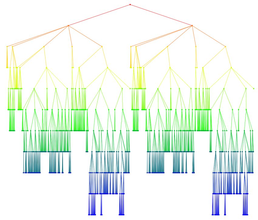
8         Beck, Burch, Munz, Di Silvestro, and Weiskopf

    Fig. 4 illustrates an n-ary branch, showing the polygon and its circumcircle.
The polygon is split into a fan of isosceles triangles using the center of the
circumcircle as splitting point. While the number of rectangles is specified by
the degree of the represented branch, the angles and lengths can be modified to
encode further information. In particular, we have two degrees of freedom:

    – Width function wx : V → R+ of rectangles—Similar to binary hierar-
      chies, the width ∆xi of a rectangle Ri can be changed, here, by modifying
      the corresponding angle αi accordingly. The angle αi should reflect weight
      wx (vi ) of a vertex vi in relation to the weight of its siblings:
                                            wx (vi )
                                αi := π · Pn              .
                                           j=1 wx (vj )

      The width of the rectangle is ∆xi := ∆x · sin α2i where ∆x is the width of
      the parent node.
    – Length stretch function wy of rectangles—Analogously, the length ∆yi
      of the rectangle Ri can be varied. This length, in contrast to the width
      ∆xi , does not underly any restrictions such as the size of a cirumcircle.
      Nevertheless, we formulate the length dependent on the length of the parent
      ∆y and the relative width sin α2i in order to consider the visual context
      (otherwise, it would be difficult to define appropriate metrics not producing
      degenerated visualizations): the length of the rectangle is ∆yi := wy (vi ) ·
      ∆y · sin α2i .

    Algorithm 2 extends Algorithm 1 and describes the generation of General-
ized Pythagoras Tree visualizations. Again, it is a recursive procedure and is
initialized by calling GeneralizedPythagorasTree(Hv , R) where Hv = (V, E)
is an arbitrary hierarchy and R = (c, ∆x, ∆y, θ) represents the initial rectan-
gle that, in contrast to the previous case, has a width ∆x and a length ∆y.
For an n-ary branching hierarchy Hv with root vertex v, the algorithm first
draws the respective rectangle before all children v1 , . . . , vn are handled: for
each child vi , the computation of angle αi forms the basis for deriving the width
∆xi and length ∆yi of the respective rectangle Ri as described above. Further-
more, the center and slope of the new rectangle need to be retrieved. Finally,
GeneralizedPythagorasTree(Hvi , Ri ) can be recursively applied to subhier-
archy Hvi having rectangle Ri as root node.
    Fig. 5 shows a sample visualization created with the algorithm. For this initial
image width function wx is set to a constant value and the length stretch function
wy is defined as 1. As a consequence, the nodes are squares again, equally sized
for each branch but n-arily branching. An example with a similar configuration
can be found in Fig. 1 (a); the same dataset is shown in Fig. 1 (b) applying
the number of leaf nodes as the width function wx . Further configurations are
discussed more systematically below. The discussion also includes the usage of
color, which, in all figures referenced so far, visualizes the depth of the nodes.
Furthermore, the order of rectangles can be modified and has an impact on
the layout; in the generalized approach, we have a higher degree of freedom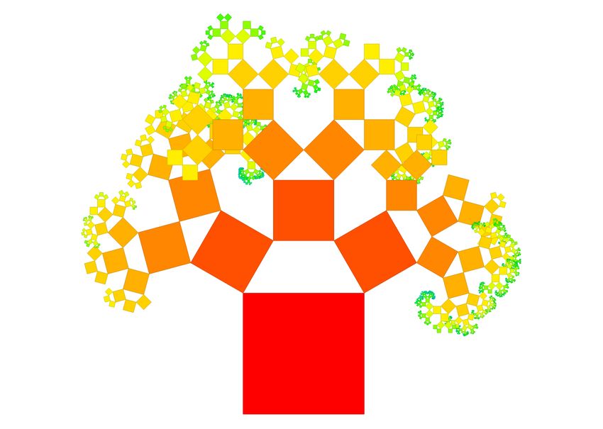
Generalized Pythagoras Trees   9

Algorithm 2 Generalized Pythagoras Tree
GeneralizedPythagorasTree(Hv , R):
 // Hv : hierarchy branching into n ∈ N0 subhierarchies Hv1 , . . . , Hvn
  // R: representative rectangle R = (c, ∆x, ∆y, θ)
    // c = (xc , yc ): center
    // ∆x, ∆y: width and length
    // θ: slope angle
  drawRectangle(R);        // draw rectangle for parent vertex
  for all Hvi do
    αi := π · Pnwx (v i)
                   wx (vj )
                            ;
                  j=1
      ∆xi := ∆x · sin α2i ;
      ∆yi := wy (vi ) · ∆y · sin α2i ;
      ci :=ComputeCenter(c, ∆x, ∆y, (α1 , . . . , αi−1 ), ∆xi , ∆yi );
      θi :=ComputeSlope(θ, (α1 , . . . , αi ));
      Ri := (ci , ∆xi , ∆yi , θi );
      GeneralizedPythagorasTree(Hvi , Ri );
  end for

(n! possibilities) than in the standard Pythagoras Trees where only a flipping
between two angles can be applied.

3.4    Excursus: Fractal Dimension

The fractal dimension is typically used as a complexity measure for fractals.
Looking back to the origin of the Generalized Pythagoras Tree visualization
and interpreting it as a fractal approach, the extended fractal approach can
be characterized by this dimension. To this end, however, not an information
hierarchy can be encoded, but the approach needs to be applied for infinite
n-arily branching structures; for simplification we do not consider scaling of
rectangles. The following analysis shows that the fractal dimension, which is
2 for traditional Pythagoras Tree fractals, asymptotically decreases to 1 for a
branching factor approaching infinity.
    Any fractal can be characterized by its fractal dimension D ∈ R that is
defined as a relation between the branching factor n and the scaling factor r
given by D = − logr n. In our scenario, we have to first compute the scaling
factor r depending on the branching factor n. Fig. 6 illustrates the following
formulas and shows an n-ary branch.
    First of all, the n-ary branch creates a convex polygon, which is split into
isosceles triangles as described before. Since all rectangles have the same width,
the angle at the tip of the triangle is α = nπ . The width of the rectangle then is

                                              α            π
                            ∆x0 = ∆x · sin      = ∆x · sin          .
                                              2            2n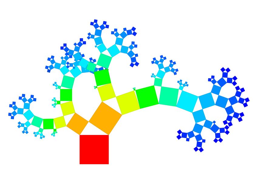
10 Beck, Burch, Munz, Di Silvestro, and Weiskopf
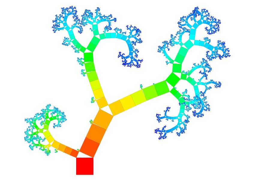
Fig. 5. Generalized Pythagoras Trees showing n-ary hierarchy using a constant width
and length stretch function.
Fig. 6. Illustrating the fractal dimension of an n-ary branching hierarchy by showing
the splitting into equally sized angles.
Relating the size of the square to the original square, the scaling factor can be
derived as follows:
∆x0 π
r= = sin .
∆x 2n
The fractal dimension finally is
log n
Dn = − π .
log sin 2n
This result confirms D2 = 2 (traditional binary branches) and shows that the
fractal dimension is approaching 1 for increasing n, i.e.,
lim Dn = 1 .
n→∞Generalized Pythagoras Trees 11
Table 1. Exploring different parameter settings such as size, order, and color of rect-
angles for a sample dataset; framed images represent the default setting and are equiv-
alent; the number of leaf nodes is applied as weight.
size
(squares) (S1) sides: weight (S2) sides: equal size (S3) sides: weight; enlarged circle
size
(rectangles) (S4) width: equal size; length: weight (S5) width: equal size; area: weight (S6) width: weight; area: weight
order
(O1) external (O2) ascending weight (O3) maximum weight in the center
color
(C1) depth (C2) weight (C3) category
3.5 Visual Parameters
The visualization approach has been described precisely but still has some de-
grees of freedom that shall be explored in the following. For example, the size of
the rectangles can be varied, the order of the subhierarchies in a branch is not
restricted, or the coloring of the nodes is open for variation. These parameters
help optimizing the layout and support the visualization by extra information
in form of weights assigned to each node. For illustrating the effect, Table 1
shows the same random hierarchy (75 nodes; maximum depth of 5) in different
parameter settings. As a weight, the number of leaf nodes is applied; but the
metric is interchangeable, for instance, by the number of subnodes, the depth of
the subtree, or a domain-specific weight. One setting (Table 1, S1 = O1 = C1),
which seemed to work most universally in our experience, is selected as default
and applied in all following figures of the paper if not indicated otherwise.
Size Already for the traditional Pythagoras Tree approach, rectangles can be
split in uniform size or non-uniform size. For the generalized approach, we define
a width function as well as a length function (Section 3.3). When employing the
same metric for both, all nodes are represented as squares. Table 1 (S1) uses the
number of leaf nodes as the common metric, which seems to be a good default
selection because more space is assigned to larger subtrees. In contrast, when all12 Beck, Burch, Munz, Di Silvestro, and Weiskopf
subnodes are assigned the same size (i.e. a constant function is employed), small
subtrees become overrepresented as depicted in Table 1 (S2). A variant of the
approach, which is shown in Table 1 (S3), extends the approach from using semi
circles to larger sectors of a circle.
Inserting different functions for width and length further increases the flexibility—
nodes are no longer squares, but differently shaped rectangles. For instance, Ta-
ble 1 (S4) encodes the number of leaf nodes in the height and applies a constant
value to the width. When defining the length function relative to the (constant)
width so that the area of the rectangle is proportional to the number of leaves,
those leaf nodes are emphasized as depicted in Table 1 (S5). A similar variant
shown in Table 1 (S6) has a constant length and chooses the width accordingly
for encoding the number of leaf nodes in the area.
Order The subnodes of an inner node of a hierarchy are visualized as an ordered
list. While, for some applications, there exist a specific, externally defined order,
many other scenarios do not dictate a specific order. In case of the latter, the
subnodes can be sorted according to a metric, which again is the number of
leaf nodes in this example. The sorting criterion mainly influences the direction
in which the diagram is growing but also influences overlapping effects. Often
the external order, at least in case it is random or independent of size, creates
quite balanced views as depicted in Table 1 (O1). When, for instance, applying
an ascending order, the image like the one shown in Table 1 (O2) grows to the
right. More symmetric visualizations such as in Table 1 (O3) are generated when
placing the vertices with the larger size in the center.
Color The areas of the rectangular nodes can be filled with color for encoding
some extra information. Selecting the color on a color scale according to the
depth of the node in the hierarchy helps comparing the depth of subtrees: for
instance, in Table 1 (C1) this encoding reveals that the leftmost main subtree,
though being shorter, is as deep as the rightmost one. Alternatively, the weight
of a node can be encoded in color like shown in Table 1 (C2), which, however, is
more suitable if the size of the node not already encodes the weight. If categories
of vertices are available, also these categories can be color-coded by discrete
colors as depicted in Table 1 (C3).
3.6 Analogy to Node-Link Diagrams
Though being derived from a fractal approach, Generalized Pythagoras Trees
can be adapted—without changing the position of nodes—to become variants
of node-link diagrams. An analogous diagram can be created as illustrated in
Fig. 7 by connecting the circle centers of the semi circles of branches by lines.
The circle centers become the nodes, the lines become the links of the resulting
node-link diagram. Like the subtrees of a Generalized Pythagoras Tree might
overlap, the analogous node-link drawing is not guaranteed to be free of edge
crossings. We prefer the Pythagoras variant over the analogous node-link variantGeneralized Pythagoras Trees 13
(a) (b) (c)
Fig. 7. Relationship between Generalized Pythagoras Trees and node-link diagrams:
(a) Generalized Pythagoras Tree; (b) Generalized Pythagoras Tree and analogous node-
link diagram; (c) analogous node-link diagram.
because it uses the available screen space more efficiently (which is important,
for instance, for color coding) and shows the width of a node explicitly.
4 Implementation
Our prototype implementation of Generalized Pythagoras Trees is written in
C++/Qt. It imports information hierarchies from text files in Newick format
or reads in directory trees from the file system. Each node can be assigned a
size that is specified in the imported file (or by the file size, in case of directory
structures). All parameters of the visualization presented can be adapted through
the user interface. For the width and length of nodes as well as for ordering and
coloring, the size metric can be employed, or alternatively, some node statistics
such as the number of subnodes or leaves. Additionally, the tool is capable of
reproducing the original fractal approach in different variants. All images of this
paper showing (Generalized) Pythagoras Trees—except for purely illustrating
figures—are generated with this tool.
The tool does not only produce static images but is interactive (Fig. 8):
Labels can be activated for larger nodes and are retrievable for all nodes by
hovering or clicking. Selecting a node shows further statistics such as the num-
ber of children, subnodes, and leaves as well as its size value. Moreover, the
tool provides geometric zooming (Fig. 8, b) as well as navigating through the
hierarchy by selecting a subhierarchy, which is then exclusively shown on screen
(Fig. 8, c); supplementary operations allow for moving a level up and jumping
back to the previous view. Nodes can be collapsed and expanded (Fig. 8, d):
a black borderline indicates collapsed nodes; the thickness encodes the size of
the collapsed subtree. For improving the readability of the current view, paths
(Fig. 8, e) and subtrees (Fig. 8, f) can be marked as well as, in case of overlap, a
subtree can be moved to front (Fig. 8, g). A search feature helps quickly finding
specific nodes (Fig. 8, h).14 Beck, Burch, Munz, Di Silvestro, and Weiskopf
(a) (b) (c) (d)
(e) (f) (g) (h)
Fig. 8. Interaction in Generalized Pythagoras Trees: (a) sample hierarchy in default
representation, (b) geometric zooming, (c) selected subhierarchy, (d) collapsed nodes,
(e) highlighted path, (f) highlighted subhierarchy, (g) subhierary moved to front, and
(h) highlighting by search.
5 Case Studies
To illustrate the usefulness of our Generalized Pythagoras Tree visualization,
we applied it to two datasets from different application domains—file systems
with file sizes as well as the NCBI taxonomy that classifies species. In these
case studies we demonstrate different parameter settings and also show how
interactive features can be applied for exploration.
5.1 File System Hierarchy
While the approach can be applied to any directory structure, we decided to
demonstrate this use case by reading in the file structure of an early version of
this particular paper. Since we use LATEX for writing, the paper directory con-
tains multiple text files including temporary files as well as a list of images. Also
included are supplementary documents and a script used for creating exemplary
random information hierarchies. All in all, the directory structure contains 139
vertices (7 directories and 132 files) having a maximum depth of 4 and a maxi-
mum branching factor of 38 (figures directory). Fig. 9 shows two visualizations
of this directory structure employing different parameter settings.
In Fig. 9 (a), we applied the default settings sizing the vertices in relation to
the number of leaf nodes and using color for encoding depth. The image shows
that, among the main directories, the figures directory contains by far the mostGeneralized Pythagoras Trees 15
(a) (b)
Fig. 9. Directory hierarchy of this paper on the file system: (a) size based on the
number of leaf nodes with color-coded depth information; (b) size encoding the file
and directory sizes with color-coded file types.
leaf nodes (94) and itself is split into three further directories, which include
the images needed for the three more complex figures and tables of this paper:
canis (Fig. 10), parameters (Table 1), and samples (Table 2). Additionally, fig-
ures also directly includes a number of images, which are needed for the other
figures. The only other directory containing a reasonable number of files is the
hierarchy generator folder; besides the generator script it contains a number of
generated sample datasets.
Customizing the parameters of the visualization for the use case of investi-
gating file systems, we assigned the file size to the size of the vertices (directory
sizes are the sum of the contained file sizes). Moreover, the file type is encoded
in the color of the vertex (category coding) a legend providing the color–type
assignments; directories are encoded in the color of the dominating file type of
the contained files. The resulting visualization as depicted in Fig. 9 (b) shows
that the figures directory is also one of the largest main directories, but there
exist other files and directories that also consume reasonable space such as the
additional material directory. Comparing the size of the main PDF document
to the images directory, it can be observed that not all image files contained in
the directory are integrated into the paper because the paper is smaller than the
images directory. The color-coded file types reveal that the most frequently oc-
curring type are PNG files, not only in the images directory but also in general.
The hierarchy generator directory mostly includes TRE files (Newick format),
but is dominated with respect to size by two TXT files (an alternative hierarchy
format not as space-efficient).16 Beck, Burch, Munz, Di Silvestro, and Weiskopf
III. Eutheria IV. Laurasiatheria
II. Amniota
I. NCBI Taxonomy
V. Carnivora
Eukaryota
cellular
organisms others
VIII. Canis Familiaris VII. Canidae VI. Caniformia
Fig. 10. NCBI taxonomy hierarchically classifying species; rectangles sizes indicate the
number of species in a subtree, color encodes the depth; an example for exploring the
taxonomy by semantic zooming is provided.
5.2 Phylogenetic Tree
Moreover, our approach is tested on a hierarchical dataset commonly used by
the biology and bioinformatics communities. The taxonomy here used has been
developed by NCBI and contains the names of all organisms that are represented
in its genetic database [4]. The specific dataset encoding the taxonomy contains
324,276 vertices (60,585 classes and 263,691 species) and has a maximum depth
of 42. The Generalized Pythagoras Tree visualization applied to this dataset
(Fig. 10 I) creates a readable overview visualization of the very complex and
large hierarchical structure. The vertices of the tree have different sizes according
to the number of leaves of their subtrees. Each inner vertex represents a class of
species and it is easy to point out the class that contains more species. The root
node is an artificial class of the taxonomy that contains every species for which
a DNA sequence or a protein is stored in the NCBI digital archive.
At the first level of the tree (see Fig. 10 I), a big node represents cellular
organisms and further nodes the Viruses, Viroids, unclassified species, and others
(this information can be retrieved by using the geometric zoom). Selecting nodes
and retrieving additional information facilitate the exploration of the tree. For
instance, the biggest node at level 2 is the Eukaryota class, which includes all
organisms whose cells contain a membrane-separated nucleus in which DNA is
aggregated in chromosomes; it still contains 177,258 of the 263,691 species.
Besides gaining an overview of the main branches of the taxonomy, the vi-
sualization tool allows for analyzing subsets of the hierarchy down to the level
of individual species by applying semantic zooming. As a concrete example, we
demonstrate the exploration process in the right part of Fig. 10; in each step
we selected the subtree of the highlighted node (red circle): Fig. 10 II showsGeneralized Pythagoras Trees 17
the Amniota class, which belongs to the tetrapoda vertebrata taxis (four-limbed
animals with backbones or spinal columns). In the next steps (Fig. 10 III-V),
we followed interesting branches until we reach the Carnivora class in Fig. 10
V, which denotes meat-eating organisms; the subtree contains 301 species. From
here, it is simple to proceed the exploration towards a well-known animal, such
as the common dog, defined as Canis Familiaris, by zooming in the subtrees
of Caniformia, literally “dog-shaped” (Fig. 10 VI), then through Canidae, the
family of dogs (Fig. 10 VII) with 45 species, and finally Canis Familiaris.
6 Discussion
The introduced technique for representing hierarchical structures is discussed by
taking existing other hierarchy visualization approaches into account. We applied
different standard hierarchy visualization techniques to a number of randomly
generated artificial datasets. The results are listed in Table 2. Each column
represents a different data set with some characteristic feature: a binary hierarchy
with a branching factor of 2, a deep hierarchy with many levels, a flat hierarchy
with a high maximum branching factor, a degenerated hierarchy that grows
linearly in depth with the number of nodes, a symmetric hierarchy having two
identical subtrees, and a self-similar hierarchy following the same pattern at
each level. The rows show standard visualization techniques in comparison to
Generalized Pythagoras Trees. Though the graphics can only act as previews
in a printed version of the paper, they are included in high resolution and are
explorable in a digital version. The following analysis considers multiple levels
of abstraction from geometry and perception to readability and aesthetics.
6.1 Geometry and Perception
Hierarchy visualizations aim at showing containment relationships between nodes
and their descendants. Considering Gestalt theory [30], different approaches exist
for visually encoding relationships: for instance, node-link diagrams use connect-
edness to express containment, while Treemaps are based on common region for
showing that several nodes belong to the same parent. In contrast, Generalized
Pythagoras Trees do neither directly draw a line between the nodes nor nest
one node into the other, but they draw rectangles of decreasing size onto an
imaginary curve. The human reader automatically connects the rectangles on
the curve, which is denoted as the law of continuation. In all hierarchy visual-
ization approaches shown in Table 2, proximity also plays a certain role (i.e.,
related nodes are placed next to each other) but should not be overinterpreted
(i.e., nodes placed next to each other are not necessarily related).
In node-link diagrams, indented tree diagrams, or icicle plots, each level in
the hierarchy creates another layer in the visualization. As a consequence, the
amount of (vertical) space available for a layer is reduced when adding further
levels. In Generalized Pythagoras Trees, however, there are no global layers for
levels of nodes: adding a level only produces a kind of local layer that is arranged18 Beck, Burch, Munz, Di Silvestro, and Weiskopf
Table 2. Comparison of hierarchy visualization approaches for representatives of a
selected set of hierarchy classes.
binary deep hierarchy flat hierarchy degenerated symmetric self-similar
hierarchy hierarchy hierarchy hierarchy
node degree of 2 high number of high maximum node linearly growing two equivalent self similar tree
hierarchy levels (25) degree (20) depth subtrees structure
node-link
indented tree
icicle plot
Treemap
Generalized
Pythagoras
TreeGeneralized Pythagoras Trees 19
on a semi circle. With respect to this characteristic, Generalized Pythagoras
Trees are similar to Treemaps, which neither have global layers but split the
area of a node for introducing the next level.
Like in icicle plots and Treemaps, larger areas are used to encode the nodes
in Generalized Pythagoras Trees. This makes it easier to use color for encoding
some metrics (such as the hierarchy level) in the nodes because colors are easier
to perceive for larger areas [29] (Color for Labeling). In contrast to Treemaps
(and complete icicle plots), Generalized Pythogoras Trees do not create space-
filling images. Areas, however, might overlap, which is discussed in detail below.
Comparing the images shown in Table 2 with respect to uniqueness, Gener-
alized Pythagoras Trees show a high visual variety: not only the subtrees vary
in size, they are also rotated. Only the splitting approach in Treemaps creates
similarly varying images, however, just with respect to texture but not shape. A
positive effect of a high visual variety is that the different datasets can be distin-
guished more easily—the visualization acts as a fingerprint. Together with the
fractal roots of the approach, the uniqueness helps detect self-similar structures:
Table 2 (last column) shows a tree having a self-similar structure, which is gen-
erated according to the same recursive, deterministic procedure for every node;
the self-similar property of the hierarchy is best detectable in the Generalized
Pythagoras Trees because every part of the tree is just a rotated version of the
complete tree.
6.2 Readability and Scalability
A hierarchy visualization is readable if the users are able to efficiently retrieve the
original hierarchical data from it and easily observe higher-level characteristics.
However, readability is also related to visual scalability, which means preserving
readability for larger datasets. While, for smaller datasets, the exact information
is usually recognizable in any hierarchy visualization, the depicted information
often becomes too detailed when increasing the scale of the dataset. The visu-
alization approach, hence, needs to use the available screen space efficiently and
has to focus on the most important information.
Generalized Pythagoras Trees clearly emphasize the higher-level nodes of the
tree (i.e., the root node and its immediate descendants): most of the area that is
filled by the visualization is consumed by these higher-level nodes, which can be
easily perceived because surrounded by whitespace. Lower-level nodes and leaf
nodes, however, become very small and are not visible. But the visualization
allows for sizing the nodes according to their importance by using the number
of leaf nodes as a metric as done in Table 2. Node-link diagrams, indented trees,
and icicle plots are similar in their focus on the higher-level nodes; as well,
lower-level nodes become difficult to discern because of lack of horizontal space.
Since the vertical space assigned to each level does not become smaller in these
visualizations, it is easier to retrieve the maximum depth of a subtree. Treemaps
focus on leaf nodes and show largely different characteristics.
The ability of a visualization technique to display also large datasets in a
readable way considerably widens its area of application. As shown in the case20 Beck, Burch, Munz, Di Silvestro, and Weiskopf
study, Generalized Pythagoras Trees can be used for browsing large hierarchies
such as the NCBI taxonomy. While it is possible to interactively explore large
hierarchies in a similar way with the other paradigms listed in Table 2, Gen-
eralized Pythagoras Trees show some characteristic scalability advantages: for
specifically deep hierarchies such as the one in the second column of Table 2,
it adaptively expands into the direction of the deepest subtree, here in spiral
shape. Comparing it to the other approaches, deep subtrees are still readable in
surprising detail. In contrast for flat hierarchies, which have a specifically high
branching factor, Generalized Pythagoras Trees do not seem to be as suitable:
the size of the nodes decreases too fast which constrains readability.
For a degenerated hierarchy (Table 2, fourth column), which grows linearly
in depth with the number of nodes, Generalized Pythagoras Trees create an
idiosyncratic but readable visualization, similar as it is the case for the other
visualization approaches. Also a symmetry in a hierarchy such as two identical
subtrees (Table 2, fifth column) can be detected: the identical tree creates the
same image, which is rotated in contrast to the other approaches, where it is
moved but not rotated.
A problem limiting the readability of Generalized Pythagoras Trees is that,
depending on the visualized hierarchy, subtrees might overlap. The other visual-
ization approaches do not share this problem; only Treemaps also employ a form
of overplotting: inner nodes are overplotted by its direct descendants. While
Treemaps use overplotting systematically, overlap only occurs occasionally in
Generalized Pythagoras Trees and is unwanted. A simple way to circumvent the
problem using the interactive tool is selecting the subset of the tree that is over-
drawn by another. Also, reordering the nodes or adapting the parameters of the
algorithm could alleviate the problem.
6.3 Aesthetics
Fractals often show similarities to natural structures such as trees, leaves, ferns,
clouds, coastlines, or mountains [23]. Among the images shown in Table 2, the
Generalized Pythagoras Trees clearly show the highest similarity to natural tree
and branching structures. Since, according to the biophilia hypothesis, humans
are drawn towards every form of life [32], this similarity suggests that Generalized
Pythagoras Trees might be considered as being specifically aesthetic. Also the
property of self-similarity that is partly preserved when generalizing Pythagoras
Trees supports aesthetics: “fractal images are usually complex, however, the
propriety of self-similarity makes these images easier to process, which gives an
explanation to why we usually find fractal images beautiful.” [19]
7 Conclusion and Future Work
In this paper, we introduced an extension of Pythagoras Tree fractals with the
goal of using these for visualizing information hierarchies. Instead of depicting
only binary trees, we generalize the approach to arbitrarily branching hierarchyGeneralized Pythagoras Trees 21
structures. An algorithm for generating these Generalized Pythagoras Trees was
introduced and the fractal characteristics of the new approach were reported.
A set of parameters allows for customizing the approach and creating a vari-
ety of visualizations. In particular, metrics can be visualized for the nodes. The
approach was implemented in an interactive tool. A case study demonstrates
the utility of the approach for analyzing large hierarchy datasets. The theoreti-
cal comparison of Generalized Pythagoras Trees to other hierarchy visualization
paradigms, on the one hand, suggested that the novel approach is capable of vi-
sualizing various features of hierarchies in a readable way comparably to previous
approaches and, on the other hand, might reveal unique characteristics of the
approach such as an increased distinguishability of the generated images and de-
tectabiltiy of self-similar structures. Further, the approach may have advantages
for visualizing deep hierarchies and provides natural aesthetics.
An open research questions is how the overplotting problem of the approach
can be solved efficiently and how the assumed advantages can be leveraged in
practical application. Moreover, formal user studies have to be conducted to
further explore the characteristics of the approach.
Acknowledgments
We would like to thank Kay Nieselt, University of Tübingen, for providing the
NCBI taxonomy dataset.
References
1. Andrews, K., Heidegger, H.: Information slices: Visualising and exploring large hi-
erarchies using cascading, semicircular disks. In: Proceedings of IEEE Symposium
on Information Visualization. pp. 9–11 (1998)
2. Balzer, M., Deussen, O., Lewerentz, C.: Voronoi treemaps for the visualization of
software metrics. In: Proceedings of Software Visualization. pp. 165–172 (2005)
3. Battista, G.D., Eades, P., Tamassia, R., Tollis, I.G.: Graph Drawing: Algorithms
for the Visualization of Graphs. Prentice-Hall (1999)
4. Benson, D.A., Karsch-Mizrachi, I., Lipman, D.J., Ostell, J., Sayers, E.W.: Gen-
bank. Nucleic Acids Research 38(suppl 1), D46–D51 (2010)
5. Bosman, A.E.: Het wondere onderzoekingsveld der vlakke meetkunde. Breda, N.V.
Uitgeversmaatschappij Parcival (1957)
6. Burch, M., Konevtsova, N., Heinrich, J., Höferlin, M., Weiskopf, D.: Evaluation of
traditional, orthogonal, and radial tree diagrams by an eye tracking study. IEEE
Transactions on Visualization and Computer Graphics 17(12), 2440–2448 (2011)
7. Burch, M., Raschke, M., Weiskopf, D.: Indented Pixel Tree Plots. In: Proceedings
of International Symposium on Visual Computing. pp. 338–349 (2010)
8. Carrière, S.J., Kazman, R.: Research report: Interacting with huge hierarchies:
beyond cone trees. In: Proceedings of Information Visualization. pp. 74–81 (1995)
9. Devroye, L., Kruszewski, P.: The botanical beauty of random binary trees. In:
Proceedings of Graph Drawing. pp. 166–177 (1995)
10. Eades, P.: Drawing free trees. Bulletin of the Institute for Combinatorics and its
Applications 5, 10–36 (1992)22 Beck, Burch, Munz, Di Silvestro, and Weiskopf
11. Grivet, S., Auber, D., Domenger, J., Melançon, G.: Bubble tree drawing algorithm.
In: Proceedings of International Conference on Computer Vision and Graphics. pp.
633–641 (2004)
12. Holton, M.: Strands, gravity, and botanical tree imaginery. Computer Graphics
Forum 13(1), 57–67 (1994)
13. Jürgensmann, S., Schulz, H.J.: A visual survey of tree visualization. IEEE Visweek
2010 Posters (2010)
14. Kleiberg, E., van de Wetering, H., van Wijk, J.J.: Botanical visualization of huge
hierarchies. In: Proceedings of Information Visualization. pp. 87–94 (2001)
15. Koike, H.: Generalized fractal views: A fractal-based method for controlling infor-
mation display. ACM Transactions on Information Systems 13(3), 305–324 (1995)
16. Koike, H., Yoshihara, H.: Fractal approaches for visualizing huge hierarchies. In:
Proceedings of Visual Languages. pp. 55–60 (1993)
17. Kruskal, J., Landwehr, J.: Icicle plots: Better displays for hierarchical clustering.
The American Statistician 37(2), 162–168 (1983)
18. Lin, C.C., Yen, H.C.: On balloon drawings of rooted trees. Graph Algorithms and
Applications 11(2), 431–452 (2007)
19. Machado, P., Cardoso, A.: Computing aesthetics. In: Advances in Artificial Intelli-
gence, Lecture Notes in Computer Science, vol. 1515, pp. 219–228. Springer Berlin
Heidelberg (1998)
20. Mandelbrot, B.: The Fractal Geometry of Nature. W.H. Freeman and Company.
New York (1982)
21. McGuffin, M., Robert, J.: Quantifying the space-efficiency of 2D graphical repre-
sentations of trees. Information Visualization 9(2), 115–140 (2009)
22. Nocaj, A., Brandes, U.: Computing Voronoi Treemaps: Faster, simpler, and
resolution-independent. Computer Graphics Forum 31(3), 855–864 (2012)
23. Peitgen, H.O., Saupe, D. (eds.): Science of Fractal Images. Springer-Verlag (1988)
24. Reingold, E., Tilford, J.: Tidier drawings of trees. IEEE Transactions on Software
Engineering 7, 223–228 (1981)
25. Rosindell, J., Harmon, L.: OneZoom: A fractal explorer for the tree of life. PLOS
Biology 10(10) (2012)
26. Schulz, H.J.: Treevis.net: A tree visualization reference. IEEE Computer Graphics
and Applications 31(6), 11–15 (2011)
27. Shneiderman, B.: Tree visualization with tree-maps: 2-D space-filling approach.
ACM Transactions on Graphics 11(1), 92–99 (1992)
28. Stasko, J.T., Zhang, E.: Focus+context display and navigation techniques for en-
hancing radial, space-filling hierarchy visualizations. In: Proceedings of the IEEE
Symposium on Information Visualization. pp. 57–65 (2000)
29. Ware, C.: Information Visualization, Second Edition: Perception for Design (Inter-
active Technologies). Morgan Kaufmann, 2nd edn. (2004)
30. Wertheimer, M.: Untersuchungen zur Lehre von der Gestalt. II. Psychological Re-
search 4(1), 301–350 (1923)
31. Wetherell, C., Shannon, A.: Tidy drawings of trees. IEEE Transactions on Software
Engineering 5(5), 514–520 (1979)
32. Wilson, E.O.: Biophilia. Harvard University Press (1984)
33. Yang, J., Ward, M.O., Rundensteiner, E.A., Patro, A.: InterRing: A visual interface
for navigating and manipulating hierarchies. Information Visualization 2(1), 16–30
(2003)You can also read