Response of early winter haze in the North China Plain to autumn Beaufort sea ice
←
→
Page content transcription
If your browser does not render page correctly, please read the page content below
Atmos. Chem. Phys., 19, 1439–1453, 2019
https://doi.org/10.5194/acp-19-1439-2019
© Author(s) 2019. This work is distributed under
the Creative Commons Attribution 4.0 License.

Response of early winter haze in the North China Plain
to autumn Beaufort sea ice
Zhicong Yin1,2 , Yuyan Li1 , and Huijun Wang1,2
1 Key Laboratory of Meteorological Disaster, Ministry of Education, Joint International Research Laboratory of Climate and
Environment Change (ILCEC)/Collaborative Innovation Center on Forecast and Evaluation of Meteorological Disasters
(CIC-FEMD), Nanjing University of Information Science & Technology, Nanjing 210044, China
2 Nansen-Zhu International Research Centre, Institute of Atmospheric Physics, Chinese Academy of Sciences, Beijing, China

Correspondence: Yuyan Li (yyan370@163.com)

Received: 30 July 2018 – Discussion started: 8 October 2018
Revised: 5 January 2019 – Accepted: 8 January 2019 – Published: 4 February 2019

Abstract. Recently, early winter haze pollution in the North     1   Introduction
China Plain has been serious and disastrous, dramatically
damaging human health and the social economy. In this            During the past few years, the increase of surface air temper-
study, we emphasized the close connection between the num-       ature has been distinctly amplified in the Arctic region and
ber of haze days in early winter in the North China Plain and    approximately twice as large as the average increase in global
the September–October sea ice in the west of the Beaufort        warming, which was called the Arctic amplification (Zhou,
Sea (R = 0.51) via both observational analyses and numer-        2017). Arctic sea ice (ASI) has decreased rapidly since the
ical experiments. Due to efficient radiative cooling, the re-    satellite era, in particular, after the year of 2000 (Gao et al.,
sponses of atmospheric circulations partially manifested as      2015). The change of ASI, associated with changed reflec-
reductions of surface wind speed over the Beaufort Sea and       tion of solar radiation and the exchange of energy and fresh
Gulf of Alaska, resulting in a warmer sea surface in the sub-    water, could remotely connect with the climate in the North-
sequent November. The sea surface temperature anomalies          ern Hemisphere, especially the winter climate in Eurasia (Liu
over the Bering Sea and Gulf of Alaska acted as a bridge.        et al., 2007; Wang and Liu, 2016). The decreased ASI over
The warmer sea surface efficiently heated the above air and      the Barents–Kara seas in late autumn stimulated a planetary-
led to suitable atmospheric backgrounds to enhance the po-       scale Rossby wave train in early winter (Honda et al., 2009;
tential of haze weather (e.g., a weaker East Asian jet stream    Kim et al., 2014) and transported its impacts to Eurasia. The
and a Rossby wave-like train propagated from North China         variation of the autumn ASI had significant impacts on the
and the Sea of Japan, through the Bering Sea and Gulf of         East Asian jet stream and the East Asian trough (Li and
Alaska, to the Cordillera Mountains). Near the surface, the      Wang, 2013) as well as the winter Arctic Oscillation (Li and
weakening sea level pressure gradient stimulated anomalous       Wang, 2012; Li et al., 2015) and the East Asian winter mon-
southerlies over the coastal area of China and brought about a   soon (Li and Wang, 2014; Li et al., 2014). Since 2000, the
calm and moist environment for haze formation. The thermal       snowfall in Siberia has been enhanced, which is probably re-
inversion was also enhanced to restrict the downward trans-      lated to the increased moisture flux from the Arctic (Cohen
portation of clear and dry upper air. Thus, the horizontal and   et al., 2012; Li and Wang, 2013). Liu et al. (2012) illustrated
vertical dispersion were both limited, and the fine particles    that the decrease of autumn ASI resulted in more block-
were apt to accumulate and cause haze pollution.                 ing patterns and water vapor, which was a benefit for heavy
                                                                 snowfall in Europe during early winter and in the United
                                                                 States during winter. Furthermore, under the positive Pacific
                                                                 Decadal Oscillation phase, the autumn ASI reduction con-
                                                                 tributed to the subseasonal variability of surface air tempera-
                                                                 ture in the East Asian winter (Xu et al., 2018; He, 2015). The

Published by Copernicus Publications on behalf of the European Geosciences Union.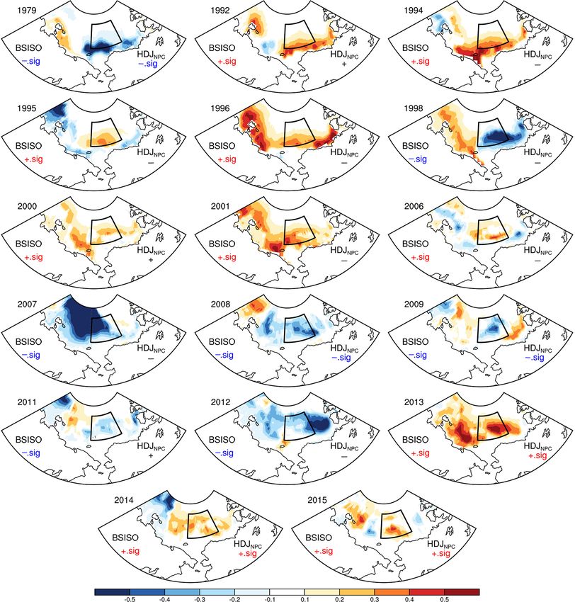
1440                                                                      Z. Yin et al.: Response of haze to Beaufort sea ice

dust (dry particles suspended in air after strong winds) and      National Meteorological Information Center, China Mete-
sandstorms (strong winds carrying sand) over North China,         orological Administration. The computing method of haze
types of weather that are sensitive to wind, also showed close    days was in accordance with Yin et al. (2017). That is, if
relationships with the variation of ASI after the mid-1990s       the visibility was lower than 10 km and the relative humidity
(Fan et al., 2017). The sea ice over the Barents–Kara seas in-    was drier than 90 %, the day was defined as 1 haze day after
duced dust-related atmospheric circulations (e.g., a strength-    filtering the other weather-affected visibility (i.e., precipita-
ened East Asian jet, increased cyclogenesis, and greater at-      tion, dust, sandstorm). The hourly PM2.5 concentration data
mospheric thermal instability).                                   were provided by the Ministry of Environmental Protection
   Haze (polluted particulate aerosols suspended in air), also    of China, including 162 sites in the North China. The daily
being sensitive to wind, frequently occurred under calm and       maximum PM2.5 was the maximum value obtained over 24 h
static weather conditions, i.e., small surface winds and strong   measurements. The 1◦ × 1◦ ERA-Interim data used here in-
thermal inversion (Yin et al., 2015; Ding and Liu, 2014; Chen     cluded the geopotential height (Z), zonal and meridional
and Wang, 2015; Cai et al., 2017; Gao and Chen, 2017).            wind, specific humidity, vertical velocity, air temperature at
For the long-term trend of the number of haze days, human         different pressure levels, sea level pressure (SLP), boundary
activities are the recognized and fundamental driver (Li et       layer height (BLH) and surface air temperature data (Dee et
al., 2018; Yang et al., 2016; Chen et al., 2019; Zhang et al.,    al., 2011). The monthly mean sea surface temperature (SST)
2018), but the rapid ASI decline also contributed to the trend    datasets, with a horizontal resolution of 1◦ × 1◦ , were also
of the number of haze days in the North China Plain after         derived from the website of ERA-Interim (Dee et al., 2011).
2000 (Wang and Chen, 2016). For the interannual to inter-         The 2.5◦ × 2.5◦ monthly reanalysis heat fluxes (i.e., the sen-
decadal variations, the impacts of ASI on the number of haze      sible heat net flux and the latent heat net flux) were available
days in the east of China were emphasized by observational        on the website of the National Center for Environmental Pre-
analyses (Wang et al., 2015) and numerical studies (Li et         diction and the National Center for Atmospheric Research
al., 2017). By the sensitive experiments, Li et al. (2017) em-    (NCAR) (Kalnay et al., 1996). The simulations from the
phasized the impacts of ASI anomalies on haze pollution in        Community Earth System Model Large Ensemble (CESM-
North China but deemphasized the role of ENSO (He et al.,         LE) datasets are employed (Kay et al., 2015). There are 35
2019). From 1979 to 2012, the ASI loss led to a northward         member ensembles in the CESM-LE simulations that com-
shift of the East Asian jet stream and weak East Asian winter     pleted at NCAR, with a horizontal resolution of 0.9◦ latitude
monsoons, indicating a strongly negative correlation with the     × 1.25◦ longitude and 30 vertical levels. The CESM-LE sim-
number of haze days in the east of China (Wang et al., 2015).     ulations were completed by the fully coupled CESM model.
However, the first mode of the empirical orthogonal function
(EOF) in Yin and Wang (2016a) presented different varia-
tions of the number of haze days in the south and north of        3   Variation of the early winter haze
the Yangtze River. The positive relationship between the au-
tumn sea ice in the Beaufort Sea and the number of haze days      In most of the observational sites in the east of China, the
in winter was briefly revealed without sufficient physical ex-    number of haze days in December and January (HDJ) ac-
planations but contributed to the prediction of the number of     counted for more than 70 % of the total number of haze days
haze days in winter (Yin and Wang, 2016b, 2017b). The num-        in winter (Fig. 1), indicating that the haze pollution in the
ber of haze days in early winter (December–January) also          early winter was more serious than that in February. Yin et
varied differently with that in February, suggesting a poten-     al. (2019) also illustrated that the interannual variation of
tially different driving mechanism. Thus, an open question        the number of haze days in February was different from that
still exists; i.e., what are the connections between Beaufort     in the early winter. Thus, it is necessary to analyze the fea-
sea ice (BSI) and the number of haze days in early winter         tures of haze pollution in the early winter and associated cli-
in the North China Plain (NCP; 34–42◦ N, 114–120◦ E), and         mate drivers. The observational HDJ were decomposed by
what are the associated physical mechanisms?                      the EOF method and the variation contribution of the first and
                                                                  second modes were 33 % and 14 %, respectively. In the first
                                                                  mode, the HDJ in the south and north of the Yangtze River
2   Datasets and methods                                          varied differently (Fig. 1) and should have a distinguishing
                                                                  relationship with the autumn ASI. In this study, we focused
The monthly sea ice concentrations (1◦ × 1◦ ) were down-          on the HDJ in the NCP region (HDJNCP , i.e., the mean of the
loaded from the Met Office Hadley Centre (Rayner et al.,          38 sites for HDJ) and their connection with the autumn ASI.
2003), which is widely used in the sea-ice-related analysis.         The HDJNCP was stable during 1979 to 1992 and de-
The number of haze days were mainly calculated with the           creased from 1993 to 2009. After 2009, the HDJNCP showed
6 h observed visibility and relative humidity. The observed       a strong upward trend. The minimum HDJNCP occurred in
relative humidity, visibility, wind speed and weather phe-        2010, which was 17.5 days. Afterwards, the HDJNCP in-
nomena data used here were collected and controlled by the        creased dramatically and persistently, reaching a maximum

Atmos. Chem. Phys., 19, 1439–1453, 2019                                            www.atmos-chem-phys.net/19/1439/2019/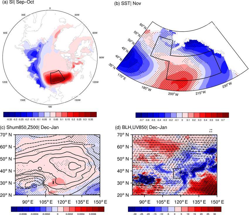
Z. Yin et al.: Response of haze to Beaufort sea ice 1441
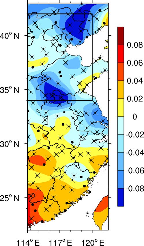
Figure 1. The spatial pattern (shading) of the first EOF mode (vari-
ation contribution: 33 %) for HDJ from 1979 to 2015. The black
crosses and dots represent the locations of the observation stations.
The cross (dot) indicates that the HDJ accounted for more (less)
than 70 % of the total winter haze days.
Figure 3. The correlation coefficient (CC) between the HDJNCP
and September–October sea ice concentration from 1979 to 2015,
after detrending. The black dots indicate CCs exceeding the 95 %
confidence level (t test). The black box represents the selected
Beaufort Sea.
4 Connection with ASI and associated physical
mechanisms
As illustrated by Wang et al. (2015), the autumn ASI signifi-
cantly and negatively affected the haze pollution in the east of
China by modulating the large-scale atmospheric circulations
and local meteorological conditions. Furthermore, the oppo-
site pattern of the number of haze days in the east of China
was revealed in Fig. 1. To confirm the response of HDJNCP to
the autumn sea ice, the correlation coefficients between the
Figure 2. The variation of (a) HDJNCP from 1979 to 2015 and HDJNCP and the September–October sea ice were assessed
(b) daily maximum PM2.5 from December to January in 2015 over after removing the linear trend (Fig. 3). A positive correla-
the NCP area. The error bars in panel (a) represent 1 standard error tion was found from the East Siberian Sea to the Beaufort
among the measured sites. Sea. In this broad region, the significantly correlated area was
intensively located over the west of the Beaufort Sea. Thus,
the area-averaged September–October sea ice area over the
(i.e., 42.7 days) in 2015. The mass concentration of PM2.5 west of the Beaufort Sea (73–80◦ N, 146–178◦ W) was cal-
is an important indicator of haze pollution. The daily maxi- culated and denoted as the BSISO index, whose correlation
mum of area-mean PM2.5 in 2015 is shown in Fig. 2b and coefficient with HDJNCP was 0.51 (above the 99 % confi-
was above 100 µg m−3 . The concentrations of PM2.5 were dence level) after removing the linear trend. This apparent
relatively lower in January 2016 than those in December positive relationship indicates that the efficient accumulation
but still exceeded the threshold of pollution in China (i.e., of the preceding autumn sea ice over the west of the Beau-
75 µg m−3 ). On 23 December, the most disastrous haze oc- fort Sea significantly intensified the number of haze days
curred, and the area-mean PM2.5 concentration approached in early winter over the NCP area. To confirm this connec-
500 µg m−3 , indicating quite poor air quality and a serious tion, the year-to-year change of the sea ice concentration was
health risk. examined (Fig. 4). From 1979 to 2015, there were 7 years
www.atmos-chem-phys.net/19/1439/2019/ Atmos. Chem. Phys., 19, 1439–1453, 2019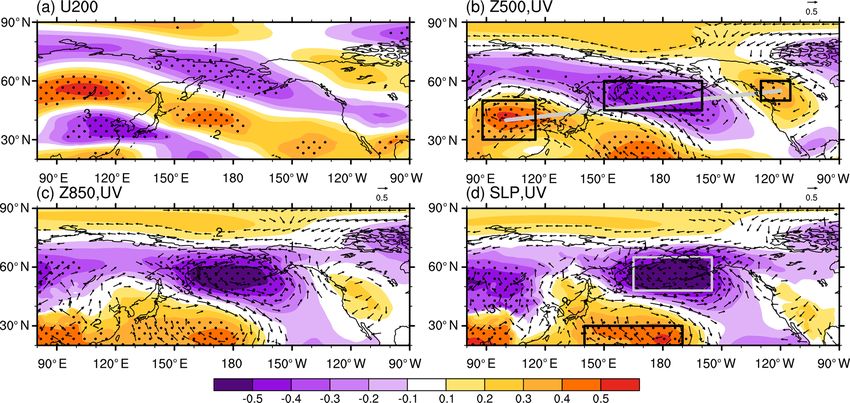
1442                                                                        Z. Yin et al.: Response of haze to Beaufort sea ice

Table 1. The correlation coefficient (CC) between the BSISO (HDJNCP ) and SST indices in October, November and December. The linear
trend was removed. The “*” indicates that the CCs exceed the 95 % confidence level, and “**” indicates that the CCs exceed the 99 %
confidence level. The meanings of the abbreviations were also explained.

                CC                                                                          Oct      Nov      Dec
                BSISO: Beaufort sea    SSTWB : SST over the west of the Beaufort Sea    −0.75∗∗   −0.26     −0.23
                ice in Sep–Oct         SSTBS : SST over the Bering Sea                     0.27    0.41∗    0.45∗∗
                                       SSTGA : SST over the Gulf of Alaska                 0.31    0.40∗    0.44∗∗
                                       SSTBA : SSTBS+ SSTGA                               0.34∗   0.43∗∗    0.48∗∗
                HDJNCP : Haze days     SSTWB : SST over the west of the Beaufort Sea     −0.30    −0.05     −0.10
                in Dec–Jan             SSTBA : SSTBS+ SSTGA                              0.52∗∗   0.61∗∗    0.56∗∗

with a significantly negative BSISO (i.e., BSISO < 0.8 × its           According to the numerical results illustrated by Deser et
standard deviation) and 10 years with a significantly posi-         al. (2007), the responses of atmospheric circulations to sea
tive BSISO (i.e., BSISO > 0.8 × its standard deviation). Dur-       ice anomalies were initially baroclinic in the first 5–10 days
ing 65 % of these years, the significant BSISO anomalies            and progressively became more barotropic and increased
corresponded to HDJNCP anomalies with the same mathe-               in both spatial extent and magnitude within 2 months. In
matical sign. There were no significantly opposite responses        September and October, due to the radiative cooling of the
of HDJNCP (| HDJNCP | > 0.8 × its standard deviation) to the        positive BSISO anomalies, the baroclinic responses of the at-
BSISO anomalies. Furthermore, the relationship seemed to            mospheric circulations manifested mainly as anomalous cy-
be enhanced after the mid-1990s. The same mathematical              clonic circulations in the upper troposphere (Fig. 6a). There
signs of the anomalies appeared more frequently.                    were also weak anticyclonic responses in the Bering Sea and
   The positive sea ice anomalies, with high albedo, can ef-        Gulf of Alaska. In the subsequent November, the extent of
ficiently reflect solar radiation and restore more fresh water,     these cyclonic and anticyclonic anomalies increased, espe-
which could influence the local and adjacent SST. The corre-        cially the anticyclonic circulations over the Bering Sea and
lation coefficients between BSISO and the simultaneous and          Gulf of Alaska (Fig. 6b). The barotropic structure of the at-
subsequent SST were computed (Fig. 5). Because of effi-             mospheric responses became more obvious; i.e., there were
cient reflections of the solar radiation, the locally negative      also cyclonic and anticyclonic circulations on both sides of
SST anomalies, located near the west of the Beaufort Sea            the Beaufort Sea, near the surface (Fig. 6d). In addition, there
(70–81◦ N, 166◦ E–138◦ W), were associated with the posi-           were also positive SLP anomalies near the Aleutian Islands,
tive BSISO anomalies in October. In the following 2 months,         indicating a weak Aleutian Low. Near the surface, a sig-
these negative SST anomalies could not be sustained; i.e.,          nificant anomalous southerly existed between cyclonic and
these anomalous responses disappeared in November. How-             anticyclonic circulations, and an anomalous east wind ex-
ever, the positive SST anomalies in the Bering Sea (49–             isted in the south of the anticyclonic circulation (Fig. 6d).
60◦ N, 165–180◦ W) and the Gulf of Alaska (40–52◦ N, 130–           Overlapping with the climate mean state, the surface wind
165◦ W) appeared in October and were persistently enhanced          speeds over the RS1 (41–54◦ N, 140–165◦ W) and RS2 (70–
in November and December. These three significantly corre-          76◦ N, 140–170◦ W) regions significantly receded (Fig. 7).
lated SSTs, located near the west of the Beaufort Sea (WB),         The area-average surface wind speed was then calculated
over the Bering Sea (BS) and the Gulf of Alaska (GA), were          and denoted as WSPDRS1 and WSPDRS2 to examine its im-
defined as SSTWB , SSTBS and SSTGA , respectively. The cor-         pacts on the simultaneous SST. In November, the climato-
relation coefficients between these three indices were enu-         logical northeasterly through the Bering Strait transported
merated in Table 1 to present the change of the correlation         cold seawater from the Arctic to the Bering Sea and re-
with SST. Over time, the linkage between BSISO and lo-              sulted in a lower SST. The correlation coefficient between
cal SST (i.e., SSTWB ) rapidly receded. To confirm the role         WSPDRS2 and SST is shown in Fig. 8 and was significantly
of the local SST on the HDJNCP , the correlation coefficient        negative in the Bering Sea. The driver of the cold seawater
between HDJNCP and SSTWB was −0.30 in October (ex-                  transportation, i.e., the surface wind, decreased and led to
ceeding the 95 % confidence level) and −0.05 and −0.10 in           warmer SSTBS in November. Another reduction of surface
the following November and December (insignificant). How-           wind speed, i.e., WSPDRS1 , indicated the weakening of the
ever, the correlation coefficients between the SSTBS (SSTGA )       west surface wind and accompanying subdued evaporation
and BSISO were persistent and even became enhanced in               near the sea surface. This RS1 region was located consis-
November and December (Table 1). We speculated that the             tently with the warmer Gulf of Alaska. The correlation co-
November SSTBS and SSTGA were the junction between the              efficients between the WSPDRS1 and SSTGA were signifi-
BSISO and HDJNCP .                                                  cantly negative, indicating that the reduction of WSPDRS1

Atmos. Chem. Phys., 19, 1439–1453, 2019                                                www.atmos-chem-phys.net/19/1439/2019/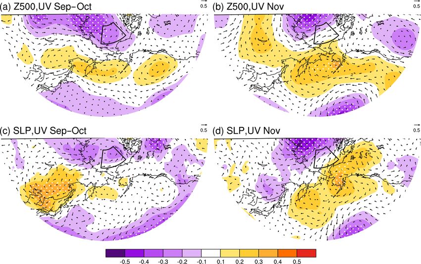
Z. Yin et al.: Response of haze to Beaufort sea ice                                                                                     1443

Figure 4. Distributions of the September–October sea ice concentration after removal of the linear trend in typical years (i.e., the year when
|BSISO| > 0.8× its standard deviation). The “+” and “−” represent the mathematical sign of the BSISO and HDJNCP indices. The “.sig”
indicates that the absolute value of the index anomaly was larger than 0.8× its standard deviation.

resulted in a warmer sea surface over the Gulf of Alaska                 and SSTGA were integrated as SSTBA to analyze their cor-
(Fig. 9a). Due to the weakening of the water evaporation, the            porate impacts on the HDJNCP . The variations of Novem-
latent heat release slowed down both in the Bering Sea and               ber SSTBA and the BSISO were strongly consistent, espe-
the Gulf of Alaska, which conserved more thermal energy                  cially after 2000 (Fig. 10). As presented in Table 1, from
on the sea surface (Fig. 9b). In addition, the upper anticy-             October, the SSTBA began to significantly connect with the
clonic circulations, with a clear sky, facilitated more short-           BSISO. Over time, this connection persisted and strength-
wave solar radiation onto the sea surface. The absorbed and              ened. The correlation coefficient between November (De-
stored thermal energy, which was connected with the posi-                cember) SSTBA and the BSISO was 0.43 (0.48), exceeding
tive BSISO anomalies, heated the sea surface over the Gulf               the 99 % significance test.
of Alaska in November, i.e., positive SSTGA anomalies. Both                 Statistically, the November SSTBA was significantly cor-
of the SSTGA and SSTBS were significantly influenced by                  related with the HDJNCP (i.e., the correlation coefficient was
the BSISO and synchronously changed. Thus, the SSTBS                     0.61 and above the 99 % confidence level), showing strong

www.atmos-chem-phys.net/19/1439/2019/                                                       Atmos. Chem. Phys., 19, 1439–1453, 2019
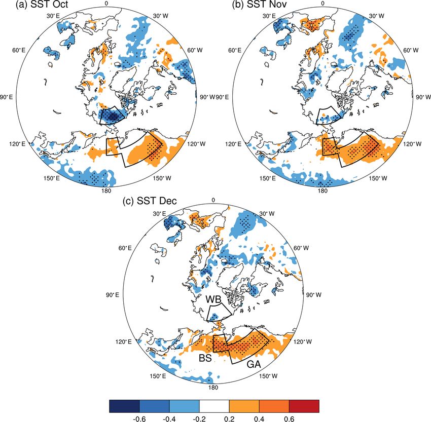
1444                                                                          Z. Yin et al.: Response of haze to Beaufort sea ice

Figure 5. The CC between the BSISO and SST in (a) October, (b) November and (c) December from 1979 to 2015, after detrending. The
black dots indicate CCs exceeding the 95 % confidence level (t test). The black boxes (WB: west of Beaufort Sea, BS: Bering Sea and GA:
Gulf of Alaska) are the significantly correlated areas, which were used to calculate the SST indices.

impacts on the number of haze days in early winter over               cated on both sides of the cyclonic circulations, i.e., over
the NCP region. To reveal the physical processes, the associ-         North China, the Sea of Japan, and the Cordillera Moun-
ated atmospheric circulations and local meteorological con-           tains. Thus, a Rossby wave-like train was induced by the
ditions were diagnosed in Figs. 11–15. The warmer sea sur-            SSTBA , which propagated from North China and the Sea of
face efficiently heated the above air and resulted in ascend-         Japan, through the Bering Sea and Gulf of Alaska, to the
ing motion from the Gulf of Alaska to the Aleutian Islands,           Cordillera Mountains. This “+–+” pattern could also be rec-
which could extend to the atmosphere at 200 hPa (Fig. 11).            ognized in the lower (Fig. 12c) and upper (Fig. 12a) tropo-
Furthermore, significant accompanying descending motions              sphere. The anticyclonic circulations over North China and
at 200 hPa were stimulated from the Sea of Okhotsk to the             the Sea of Japan were recognized as the key atmospheric
Hawaiian Islands (Fig. 11a). Near the surface, there was also         system to influence the haze pollution in the NCP area (Yin
a sinking motion over the Hawaiian Islands (Fig. 11b). On the         and Wang, 2016a; Yin et al., 2017). To confirm the linkage
mid-troposphere, the significantly negative Z500 anomalies,           between this Rossby wave-like train and SSTBA , the area-
i.e., cyclonic circulations, were exerted above the warmer            averaged Z500 in three centers (30–50◦ N, 88–115◦ E; 45–
Bering Sea and Gulf of Alaska (Fig. 12b). The responses               60◦ N, 150◦ E–160◦ W; 50–60◦ N, 115–130◦ W) were calcu-
of the December–January atmospheric circulations to the               lated and are shown in Fig. 13. The correlation coefficients
warmer November SSTBA showed deeply barotropic struc-                 between the three centers, from west to east, with SSTBA
tures. There were also significant cyclonic circulations in the       were 0.47, −0.46 and 0.37, all above the 95 % confidence
lower troposphere (Fig. 12c) and near the surface (Fig. 12d).         level. Due to the change of the pressure gradient, there were
At 500 hPa, there were significant anticyclonic anomalies lo-         positive zonal westerlies from Lake Baikal to the Hawai-

Atmos. Chem. Phys., 19, 1439–1453, 2019                                                 www.atmos-chem-phys.net/19/1439/2019/
Z. Yin et al.: Response of haze to Beaufort sea ice                                                                              1445

Figure 6. The CC between BSISO and September–October (a) geopotential height (shading), wind (arrow) at 500 hPa, (c) SLP (shade) and
surface wind (arrow) and between BSISO and November (b) geopotential height (shading), wind (arrow) at 500 hPa, (d) SLP (shade) and
surface wind (arrow) from 1979 to 2015, after detrending. The white dots indicate CCs exceeding the 90 % confidence level (t test). The
black box in panels (a)–(d) represents the location of the Beaufort Sea.

                                                                      Figure 8. The CC between WSPDRS2 and SST in November from
Figure 7. The distribution of the climate mean surface wind (ar-      1979 to 2015. The black dots indicate that the CCs exceeded the
row) in November and the CC between the BSISO and surface wind        95 % confidence level (t test). The black box represents the BA
speed in November from 1979 to 2015, after detrending. The black      (Bering Sea–Gulf of Alaska). The linear trend was removed.
dots indicate CCs exceeding the 95 % confidence level (t test). The
black boxes (RS1 and RS2) are the significantly correlated areas,
which were used to calculate the WSPDRS1 and WSPDRS2 index.

                                                                      Asian major trough, which reached the NCP area and guided
ian Islands and negative westerly anomalies from eastern              cold air southward, was truncated by the anomalous anticy-
China to the west subtropical Pacific (Fig. 12a). Therefore,          clonic circulations (Fig. 12b). In contrast, due to the cyclonic
zonal west winds prevailed in the mid-high latitudes, and             anomalies over the Aleutian area, the northern section of the
the meridionality of the atmosphere was reduced. The East             East Asian major trough was enhanced but moved eastward.
Asia jet stream was weakened by anomalous easterlies and              These large-scale anomalous atmospheric circulations could
shifted northwards, indicating a decrease of the southward            provide a suitable background for the enhancement of the
cold air activities. In addition, the southern section of the East    potential of the haze weather (Yin and Wang, 2017a).

www.atmos-chem-phys.net/19/1439/2019/                                                  Atmos. Chem. Phys., 19, 1439–1453, 2019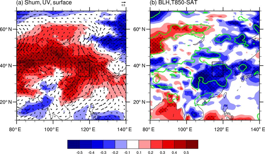
1446                                                                          Z. Yin et al.: Response of haze to Beaufort sea ice

Figure 9. The CC between WSPDRS1 and (a) SST and (b) latent heat flux in November from 1979 to 2015. The black dots indicate that the
CCs exceeded the 95 % confidence level (t test). The black box represents the BA area. The linear trend was removed.

                                                                     cles, which reduced the visibility rapidly and structured sta-
                                                                     ble weather conditions. The surface wind speed, indicating
                                                                     the horizontal dispersion capacity of the atmosphere, also
                                                                     subsided. In addition, the shallow thermal inversion layer or
                                                                     the boundary layer limited the upward dispersion of the pol-
                                                                     lutant particles. As shown in Fig. 14b, the intensity of the
                                                                     thermal inversion over the NCP area was significantly height-
                                                                     ened while the boundary layer significantly declined. Gener-
                                                                     ally, the air on the high altitude was relatively dry and clean.
Figure 10. The variation of the normalized BSISO (blue) and          The sinking of the upper air to the surface was an impor-
November SSTBA (green) from 1979 to 2015, after detrending.          tant approach in dispersing the surface pollution (Sun et al.,
                                                                     2017). Instead, the upward motion above the boundary layer
                                                                     resisted the breaking of the thermal layer and was in favor
   Near the surface, because of the SSTBA heating, the Aleu-         of haze occurrence (Fig. 15a). The associated anomalous de-
tian Low moved eastward and was enhanced over the Bering             scending flow was blocked in the north of 46◦ N, which was
Sea and Gulf of Alaska. Consistent with the barotropic               consistent with the location of the northward cold air activi-
anomalies in the above air, there were positive SLP anoma-           ties (Fig. 15a). Influenced by the warmer SSTBA , there were
lies from Northeast China to the West Pacific (Fig. 12d).            anomalous ascending motions over the NCP area. Thus, the
That is, a north–south seesaw over the North Pacific was dis-        weakened downward transportation of momentum was not
cerned clearly, similar to the anomalous North Pacific Os-           sufficient to enhance the winds near the surface and break
cillation (NPO) pattern (Rogers, 1981). The difference of            the thermal inversion layer. Therefore, the clear, dry and cold
SLP (20–30◦ N, 140◦ E–170◦ W minus 48–65◦ N, 165◦ E–                 air was difficult to transport to the surface, indicating the fail-
155◦ W) was calculated to quantify this seesaw pattern,              ure of the blowing wind. Under poor ventilation conditions,
whose correlation coefficients with the BSISO, SSTBA and             i.e., the horizontal and vertical dispersion was limited, the
HDJNCP were 0.33, 0.64 and 0.61, respectively. Bounded               fine particles were apt to accumulate and cause haze pollu-
by the east of China, the south positive center of NPO and           tion. Combined with favorable moisture conditions, the haze
the negative anomalies occupied the West Pacific and Eura-           exacerbated rapidly and perniciously.
sia, respectively. The drivers of the East Asian winter mon-
soon, i.e., the pressure gradient between the continent and
the ocean, became weak, indicating the limitation of cold            5   Causality verification by CESM-LE experiments
air and ventilation conditions. Compared to the local zonal
wind, the meridional wind played more important roles on             The connection between the haze pollution in North China
weakening the horizontal dissipation conditions of the air.          and ASI and associated physical mechanisms were statisti-
The southerly anomalies were located over the coastal area of        cally analyzed in the above sections. To confirm the causal-
China and transported moisture to the NCP area (Fig. 14a),           ity, numerical experiments were designed with the public
providing moist air for haze formation. In winter, the anoma-        CESM-LE datasets. To be consistent with the observational
lous south winds also weakened the prevailing northerlies            results, the variables from CESM-LE from 1979 to 2015 are
and reduced the invasion of cold air. The humid atmosphere           employed, which were combined by the historical simula-
was conducive to the hygroscopic growth of pollutant parti-          tion during 1979–2005 and the data during 2006–2015 from

Atmos. Chem. Phys., 19, 1439–1453, 2019                                                www.atmos-chem-phys.net/19/1439/2019/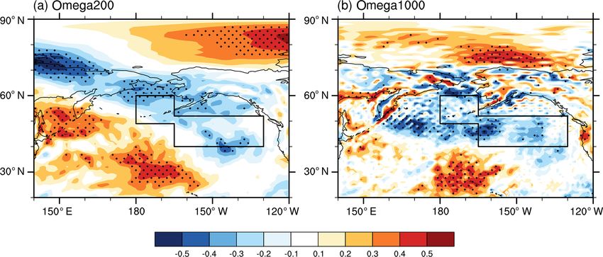
Z. Yin et al.: Response of haze to Beaufort sea ice                                                                                   1447

Figure 11. The CC between November SSTBA and (a) omega (vertical velocity) at 200 hPa and (b) at 1000 hPa in December and January
from 1979 to 2015. The black dots indicate that the CCs exceeded the 95 % confidence level (t test). The linear trend was removed. The black
box represents the BA area.

Figure 12. The CC between the November SSTBA and (a) zonal wind at 200 hPa, (b) wind (arrow), geopotential height (shading) at 500 hPa,
(c) wind (arrow), geopotential height (shading) at 850 hPa, (d) surface wind (arrow) and SLP (shading) in December–January from 1979 to
2015. The black dots indicate that the CCs exceeded the 95 % confidence level (t test). The linear trend was removed. The black boxes in
panel (b) represent the three anomalous centers at 500 hPa, and the gray and black boxes in panel (d) represent the negative and positive
anomalous centers.

                                                                        the Representative Concentration Pathway 8.5 forcing simu-
                                                                        lation. A total of 35 CESM-LE ensemble members were used
                                                                        here. The CESM-LE simulations were completed by the fully
                                                                        coupled CESM model; thus the interactions among sea ice,
                                                                        sea temperature and atmosphere can be contained. The years
                                                                        when the sea ice anomalies concentrated in the west of the
                                                                        Beaufort Sea were selected, and the differences between the
                                                                        positive BSISO and negative BSISO years were be identified
                                                                        as the responses to the sea ice anomalies. In the numerical
Figure 13. The variation of the November normalized SSTBA (gray         experiment, all available CESM-LE members were included
bar) and area-averaged geopotential height at 500 hPa of the three      and different amplitudes of sea ice anomalies were compos-
anomalous centers (west: black, middle: green, east: orange) from       ited; thus the uncertainty from the internal variability were
1979 to 2015, after detrending.                                         largely reduced.

www.atmos-chem-phys.net/19/1439/2019/                                                      Atmos. Chem. Phys., 19, 1439–1453, 2019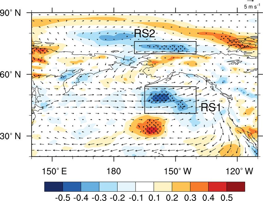
1448                                                                              Z. Yin et al.: Response of haze to Beaufort sea ice

Figure 14. The CC between the November SSTBA and (a) surface wind (arrow), specific humidity (Shum, shading) at 1000 hPa, (b) BLH
(shading) and thermal inversion potential (contour) from 1979 to 2015. The black dots indicate that the CCs exceeded the 90 % confidence
level, and the solid (dashed) green lines indicate that the positive (negative) correlations exceeded the 90 % confidence level (t tests). The
linear trend was removed. The black boxes represent the NCP area. The thermal inversion potential was defined as the air temperature at
850 hPa minus SAT.

Figure 15. The cross section (114–120◦ E mean) CC of (a) the HDJNCP and (b) November SSTBA for omega (shading) and wind (arrow)
in December–January from 1979 to 2015. The black dots indicate that the CCs exceeded the 95 % confidence level (t test). The linear trend
was removed.

  In Fig. 16a, the sea ice anomalies were obvious in the                 circulations with regard to anomalous BSISO, the composite
key region. The maximum of the difference in sea ice con-                difference was also consistent with the observed results. The
centration was more than 35 % (Fig. 16a). In the following               anticyclonic anomalies of the geopotential height at 500 hPa
November, the accumulated sea ice favored increased SST                  were also well reproduced by the numerical model in the
over the Gulf of Alaska (Fig. 16b), which is in good accor-              early winter (Fig. 16c). In the lower troposphere, there were
dance with the observed results. Although there were weaker              also anomalous anticyclones over North China and Northeast
but negative SST responses in the Bering Sea, the positive               China, which induced anomalous southerlies (Fig. 16d) and
SST anomalies extended southwards and enhanced the air–                  weakened the cold air from the high latitudes. Furthermore,
sea interaction. In terms of the corresponding atmospheric               the moist air condition (Fig. 16c) and lower boundary layer

Atmos. Chem. Phys., 19, 1439–1453, 2019                                                     www.atmos-chem-phys.net/19/1439/2019/
Z. Yin et al.: Response of haze to Beaufort sea ice 1449
Figure 16. Composite difference of (a) September–October sea ice concentration, (b) sea surface temperature in November, (c) geopotential
height (contour) at 500 hPa, surface specific humidity in December–January, (d) BLH (shading) and surface wind (arrow) in December–
January. The black box in panel (a) represents the location of the Beaufort Sea, and in panel (b) it represents the BA area. Results are based
on 35 ensembles of CESM-LE simulations. The black dots indicate that the mathematical sign of the changes with shading from more than
50 % of the members are consistent with the ensemble mean.
(Fig. 16d) were also verified to be significantly connected 6 Conclusions and discussions
with the positive BSISO anomalies. Consistent with the ob-
served results, the linkages between the BSISO and the haze In the subseasonal scale, the haze weather in early winter oc-
pollution in the North China also exist in CESM-LE simu- curred more frequently and varied differently from that in
lations. Meanwhile, the corresponding physical mechanisms February. In this study, the close relationship between the
were also well reproduced by the large ensemble members. number of haze days in early winter in the NCP area and
The performances of numerical models in the mid-high lat- the September–October sea ice in the west of the Beaufort
itudes were consistently limited; however, the results from Sea, with a correlation coefficient of 0.51, was revealed. The
CESM-LE here successfully captured major features and positive September–October sea ice anomalies over the west
general physical processes as expected. Consequently, the of the Beaufort Sea strongly intensified the early winter haze
robustness of the proposed connections and physical mecha- pollution over the NCP area, or more precisely, increased the
nisms were strongly confirmed. number of haze days. Associated physical mechanisms were
further examined. Due to the high albedo and efficient re-
flections, the local SST in October became cooler than the
climate mean state, showing the radiative cooling effect. The
responses of the atmospheric circulations initially manifested
as anomalous cyclonic circulations in the upper troposphere
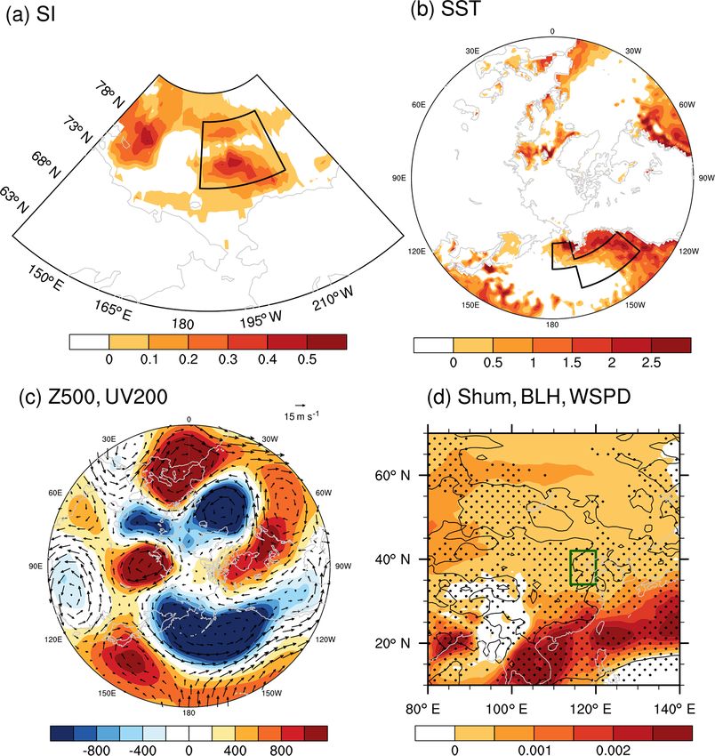
www.atmos-chem-phys.net/19/1439/2019/ Atmos. Chem. Phys., 19, 1439–1453, 20191450 Z. Yin et al.: Response of haze to Beaufort sea ice Figure 17. The distributions of (a) September–October sea ice concentration in 2015, (b) sea surface temperature in November 2015, (c) geopotential height (shading) at 500 hPa, wind (arrow) at 200 hPa in December–January 2015, (d) specific humidity (shading) at 1000 hPa, BLH (black dots indicate that its value is negative) and WSPD (contour, solid black lines indicate a negative value) in December–January 2015. The black box in panel (a) represents the location of the Beaufort Sea, and in panel (b) it represents the BA area. The linear trend was removed. and then developed into cyclonic and anticyclonic circula- west wind anomalies prevailed in the mid-high latitudes, and tions on both sides of the Beaufort Sea in the subsequent the meridionality of the atmosphere was reduced, indicat- November. The decreased surface wind through the Bering ing the decrease of the southward cold air activities. A +– Strait could not transport cold seawater to the Bering Sea as + Rossby wave-like train propagated from North China and usual and led to a warmer sea surface over the Bering Sea. the Sea of Japan, through the Bering Sea and Gulf of Alaska, The reduction of surface wind speed over the Gulf of Alaska to the Cordillera Mountains. Near the surface, the NPO-like weakened the seawater evaporation and the latent heat re- pattern and the negative SLP anomalies over Eurasia induced lease, which conserved more thermal energy in the sea sur- southerly anomalies over the coastal area of China, provid- face, i.e., positive SST anomalies. ing a calm and moist environment for haze formation. In ad- The November SST anomalies over the Bering Sea and dition, the intensity of the thermal inversion over the NCP Gulf of Alaska acted as a bridge in the close relationship be- area was significantly enhanced, and the clear, dry and cold tween the BSISO (R = 0.43, exceeding the 99 % confidence air was difficult to transport to the surface. The horizontal level) and HDJNCP (R = 0.61). The warmer sea surface ef- and vertical dispersions were both limited, so the fine parti- ficiently heated the air above and resulted in significant re- cles were apt to accumulate and cause haze pollution. The sponses in the atmosphere. In the upper troposphere, zonal linkages and corresponding physical mechanisms were well Atmos. Chem. Phys., 19, 1439–1453, 2019 www.atmos-chem-phys.net/19/1439/2019/
Z. Yin et al.: Response of haze to Beaufort sea ice                                                                                 1451

reproduced via the large CESM-LE ensembles, confirming              Interim, 2018). The monthly heat flux data are available from
the causality.                                                      the NCEP/NCAR data archive: http://www.esrl.noaa.gov/psd/data/
   In this study, the response of the number of haze days in        gridded/data.ncep.reanalysis.html (NCEP/NCAR, 2018). The sim-
early winter in the North China Plain to the autumn Beaufort        ulation data are available from the Community Earth System
sea ice and the associated physical mechanisms were inves-          Model Large Ensemble datasets (2018): http://www.cesm.ucar.edu/
                                                                    projects/community-projects/LENS/data-sets.html.
tigated. As shown in Fig. 2, the HDJNCP was 42.7 days and
reached its maximum in 2015. Thus, the measurements in
2015 were composited after removing the linear trend to ver-
                                                                    Author contributions. ZY and HW thought of the idea, ZY and YL
ify the results from the observational analyses (Fig. 17). In
                                                                    created the figures, and ZY wrote the manuscript.
September–October 2015, there were positive sea ice anoma-
lies on the west of the Beaufort Sea (Fig. 17a), which sat-
isfied the close relationship revealed in this study. Mean-         Competing interests. The authors declare that they have no conflict
while, an obviously warmer SST in November was observed             of interest.
in most of the BA region (Fig. 17b), transferring the impacts
of the BSISO. As a result, a weaker East Asia jet stream,
an anomalous southerly (Fig. 17c), limited horizontal and           Acknowledgements. This research was supported by the Na-
vertical dispersion conditions, and moist air (Fig. 17d) en-        tional Natural Science Foundation of China (41705058 and
hanced the early winter haze pollution in 2015. However,            91744311), the National Key Research and Development Plan
some questions remain unanswered and should be inves-               (2016YFA0600703), the CAS–PKU Partnership program, and the
tigated with numerical models in future work. For exam-             funding of the Jiangsu Innovation and Entrepreneurship team.
ple, the internal dynamic and thermal processes and how
the positive sea ice anomalies (radiative cooling) affected         Edited by: Jianping Huang
                                                                    Reviewed by: two anonymous referees
the atmospheric circulations are not fully understood. Dur-
ing this work, linear correlation analyses were the main re-
search technique, and a linear relationship was discovered.
In fact, the dynamic–thermodynamic processes in the air–ice
interaction are neither straightforward nor necessarily linear      References
(Zhang et al., 2000; Gao et al., 2015). Considering the contra-
                                                                    Cai, W. J., Li, K., Liao, H., Wang, H. J., and Wu, L. X.:
diction among the results by a single numerical model (Gao            Weather Conditions Conducive to Beijing Severe Haze More
et al., 2015), a multi-model ensemble was required to solve           Frequent under Climate Change, Nat. Clim. Change, 7, 257–262,
the internal physical mechanisms. Furthermore, the Novem-             https://doi.org/10.1038/nclimate3249, 2017.
ber SST anomalies over the Bering Sea and Gulf of Alaska            Chen, H. P. and Wang, H. J.: Haze Days in North China and
were treated as a bridge to connect the sea ice and the haze          the associated atmospheric circulations based on daily visibil-
pollution. It is necessary to examine whether this bridge was         ity data from 1960 to 2012, J. Geophys. Res., 120, 5895–5909,
constructed all the time. Particularly, after 2010, haze pollu-       https://doi.org/10.1002/2015JD023225, 2015.
tion became more serious. The driven role of the BSISO and          Chen, H., Wang, H., Sun, J., Xu, Y., and Yin, Z.: Anthropogenic
the bridge of SSTBA needs to be verified. Moreover, as re-            fine particulate matter pollution will be exacerbated in eastern
                                                                      China due to 21st century GHG warming, Atmos. Chem. Phys.,
vealed by the EOF decomposition, the number of haze days
                                                                      19, 233–243, https://doi.org/10.5194/acp-19-233-2019, 2019.
in southern China varied differently. Its relationship with the
                                                                    CMA: Ground observations, available at: http://data.cma.cn/, last
sea ice in the Arctic is still unclear and needs to be addressed.     access: 3 April 2018.
The significant relationship revealed in this study and associ-     Cohen, J. L., Furtado, J. C., Barlow, M. A., Alexeev, V. A.,
ated previous work potentially improved the monthly predic-           and Cherry, J. E.: Arctic warming, increasing snow cover and
tion of haze pollution. Valuable haze predictions are urgently        widespread boreal winter cooling, Environ. Res. Lett., 7, 014007,
needed by the scientific decision-making departments to con-          https://doi.org/10.1088/1748-9326/7/1/014007, 2012.
trol haze pollution in China (Wang, 2018).                          Community Earth System Model Large Ensemble datasets:
                                                                      http://www.cesm.ucar.edu/projects/community-projects/LENS/
                                                                      data-sets.html, last access: 14 December 2018.
Data availability. Sea ice concentration data can be downloaded     Dee, D. P., Uppala, S. M., Simmons, A. J., Berrisford, P., Poli,
from the Met Office Hadley Centre: https://www.metoffice.gov.         P., Kobayashi, S., Andrae, U., Balmaseda, M. A., Balsamo,
uk/hadobs/hadisst/data/download.html (Met Office Hadley Cen-          G., Bauer, P., Bechtold, P., and Beljaars, A. C. M.: The ERA-
tre, 2018). The ground observations are from the website: http:       Interim reanalysis: configuration and performance of the data
//data.cma.cn/ (CMA, 2018). The atmospheric composition data          assimilation system, Q. J. Roy. Meteor. Soc., 137, 553–597,
can be obtained from the authors. Atmospheric data and land           https://doi.org/10.1002/qj.828, 2011.
surface data are available on the ERA-Interim website: http://      Deser, C., Tomas, R. A., and Peng, S.: The transient atmospheric
www.ecmwf.int/en/research/climate-reanalysis/era-interim (ERA-        circulation response to north atlantic sst and sea ice anomalies, J.
                                                                      Climate, 20, 4751, https://doi.org/10.1175/JCLI4278.1, 2007.

www.atmos-chem-phys.net/19/1439/2019/                                                 Atmos. Chem. Phys., 19, 1439–1453, 2019
1452 Z. Yin et al.: Response of haze to Beaufort sea ice
Ding, Y. H. and Liu, Y. J.: Analysis of long-term variations of fog Li, F. and Wang, H. J.: Autumn Eurasian snow depth, autumn Arctic
and haze in China in recent 50 years and their relations with at- sea ice cover and East Asian winter monsoon, Int. J. Climatol.,
mospheric humidity, Sci. China Ser. D: Earth Sci., 57, 36–46, 34, 3616–3625, https://doi.org/10.1002/joc.3936, 2014.
2014 (in Chinese). Li, F., Wang, H. J., and Gao, Y. Q.: On the strengthened relationship
ERA-Interim: Atmospheric data, available at: http://www.ecmwf. between East Asian winter monsoon and Arctic Oscillation: A
int/en/research/climate-reanalysis/era-interim, last access: 7 comparison of 1950–1970 and 1983–2012, J. Climate, 27, 5075–
May 2018. 5091, https://doi.org/10.1175/JCLI-D-13-00335.1, 2014.
Fan, K., Xie, Z. M., Wang, H. J., Xu, Z. Q., and Liu, J. P.: Fre- Li, F., Wang, H. J., and Gao, Y. Q.: Change in Sea Ice Cover
quency of spring dust weather in North China linked to sea is Responsible for Non-Uniform Variation in Winter Temper-
ice variability in the Barents Sea, Clim. Dynam., 51, 4439, ature over East Asia, Atmos. Oceanic Sci. Lett., 8, 376–382,
https://doi.org/10.1007/s00382-016-3515-7, 2017. https://doi.org/10.3878/AOSL20150039, 2015.
Gao, Y. and Chen, D.: A dark October in Beijing 2016, Atmos. Li, K., Liao, H., Cai, W., and Yang, Y.: Attribution of anthropogenic
Oceanic Sci. Lett., 10, 206–213, 2017. influence on atmospheric patterns conducive to recent most se-
Gao, Y. Q., Sun, J. Q., Li, F., He, S. P., Sandven, S., Yan, Q., vere haze over eastern China, Geophys. Res. Lett., 45, 2072–
Zhang, Z. S., Lohmann, K., Keenlyside, N., Furevik, T., and 2081, https://doi.org/10.1002/2017GL076570, 2018.
Sou, L. L.: Arctic Sea Ice and Eurasian Climate: A Review, Li, S. L., Han, Z., and Chen, H. P.: A Comparison of the Effects of
Adv. Atmos. Sci., 32, 92–114, https://doi.org/10.1007/s00376- Interannual Arctic Sea Ice Loss and ENSO on Winter Haze Days:
014-0009-6, 2015. Observational Analyses and AGCM Simulations, J. Meteor. Res.,
He, C., Liu, R., Wang, X. M., Liu, S. C., Zhou, T. J., 31, 820–833, https://doi.org/10.1007/s13351-017-7017-2, 2017.
and Liao, W. H.: How does El Niño-Southern Oscillation Liu, J. P., Zhang, Z. H., Horton, R. M., Wang, C. Y., and
modulate the interannual variability of winter haze days Ren, X. B.: Variability of North Pacific Sea Ice and East
over eastern China?, Sci. Total Environ., 651, 1892–1902, Asia North Pacific Winter Climate, J. Climate, 20, 1991–2001,
https://doi.org/10.1016/j.scitotenv.2018.10.100, 2019. https://doi.org/10.1175/JCLI4105.1, 2007.
He, S. P.: Asymmetry in the Arctic Oscillation Teleconnection with Liu, J. P., Curry J. A., Wang, H. J., Song, M., and Horton, R. M.:
January Cold Extremes in Northeast China, Atmos. Oceanic Impact of declining Arctic sea ice on winter snowfall, P. Natl.
Sci. Lett., 8, 386–391, https://doi.org/10.3878/AOSL20150053, Acad. Sci. USA, 109, 4074–4079, 2012.
2015. Met Office Hadley Centre: Sea ice cover data, available at: https://
Honda, M., Inoue, J., and Yamane, S.: Influence of low Arctic sea www.metoffice.gov.uk/hadobs/hadisst/data/download.html, last
ice minima on anomalously cold Eurasian winters, Geophys. access: 5 April 2018.
Res. Lett., 36, L08707, https://doi.org/10.1029/2008GL037079, NCEP/NCAR: heat fluxes data, available at: http://www.esrl.noaa.
2009. gov/psd/data/gridded/data.ncep.reanalysis.html, last access: 10
Kalnay, E., Kanamitsu, M., Kistler, R., Collins, W., Deaven, D., April 2018.
Gandin, L., Iredell, M., Saha, S., White, G., Woollen, J., Zhu, Y., Rayner, N. A., Parker, D. E., Horton, E. B., Folland, C. K., Alexan-
Leetmaa, A., Reynolds, R., Chelliah, M., Ebisuzaki, W., Higgins, der, L. V., Rowell, D. P., Kent, E. C., and Kaplan, A.: Global
W., Janowiak, J., Mo, K. C., Ropelewski, C., Wang, J., Jenne, R., analyses of sea surface temperature, sea ice, and night marine air
and Joseph, D.: The NCEP/NCAR 40-year reanalysis project, B. temperature since the late nineteenth century, J. Geophys. Res.,
Am. Meteorol. Soc., 77, 437–471, https://doi.org/10.1175/1520- 108, 4407, https://doi.org/10.1029/2002JD002670, 2003.
0477(1996)0772.0.CO;2, 1996. Rogers, J. C.: The North Pacific Oscillation, Int. J. Climatol., 1, 39–
Kay, J. E., Deser, C., Phillips, A., Mai, A., Hannay, C., Strand, 57, https://doi.org/10.1002/joc.3370010106, 1981.
G., Arblaster, J., Bates, S., Danabasoglu, G., Edwards, J., Hol- Sun, X. C., Han, Y. Q., Li, J., Kang, G. H., and Wang, B. M.: Anal-
land, M., Kushner, P., Lamarque, J.-F., Lawrence, D., Lind- ysis of the Influence of Vertical Movement on the Process of Fog
say, K., Middleton, A., Munoz, E., Neale, R., Oleson, K., and Haze with Air Pollution, Plateau Meteorology, 36, 1106–
Polvani, L., and Vertenstein, M.: The Community Earth Sys- 1114, 2017 (in Chinese).
tem Model (CESM) Large Ensemble Project: A community re- Wang, H. J., Chen, H. P., and Liu J. P.: Arctic sea ice decline inten-
source for studying climate change in the presence of inter- sified haze pollution in eastern China, Atmos. Oceanic Sci. Lett.,
nal climate variability, B. Am. Meteorol. Soc., 96, 1333–1349, 8, 1–9, 2015.
https://doi.org/10.1175/BAMS-D-13-00255.1, 2015. Wang, H.-J. and Chen, H.-P.: Understanding the recent trend of
Kim, B. M., Son, S. W., Min, S. K., Jeong, J. H., Kim, S. J., Zhang, haze pollution in eastern China: roles of climate change, At-
X. D., Shim, T., and Yoon, J. H.: Weakening of the stratospheric mos. Chem. Phys., 16, 4205–4211, https://doi.org/10.5194/acp-
polar vortex by Arctic sea-ice loss, Nat. Commun., 5, 4646, 16-4205-2016, 2016.
https://doi.org/10.1038/ncomms5646, 2014. Wang, H. J.: On assessing haze attribution and control mea-
Li, F. and Wang, H. J.: Autumn sea ice cover, winter northern hemi- sures in China, Atmos. Oceanic Sci. Lett., 11, 120–122,
sphere annular mode, and winter precipitation in Eurasia, J. Cli- https://doi.org/10.1080/16742834.2018.1409067, 2018.
mate, 26, 3968–3981, 2012. Wang, S. Y. and Liu, J. P.: Delving into the relationship be-
Li, F. and Wang, H. J.: Relationship between Bering sea ice cover tween autumn Arctic sea ice and central–eastern Eurasian
and East Asian winter monsoon Year-to-Year Variations, Adv. winter climate, Atmos. Oceanic Sci. Lett., 9, 366–374,
Atmos. Sci., 30, 48–56, 2013. https://doi.org/10.1080/16742834.2016.1207482, 2016.
Xu, X. P., Li, F., He, S. P., and Wang, H. J.: Subseasonal reversal
of East Asian surface temperature variability in winter 2014/15,
Atmos. Chem. Phys., 19, 1439–1453, 2019 www.atmos-chem-phys.net/19/1439/2019/Z. Yin et al.: Response of haze to Beaufort sea ice 1453 Adv. Atmos. Sci., 35, 737–752, https://doi.org/10.1007/s00376- Yin, Z., Wang, H., and Chen, H.: Understanding severe win- 017-7059-5, 2018. ter haze events in the North China Plain in 2014: roles Yang, Y., Liao, H., and Lou, S.: Increase in winter haze over east- of climate anomalies, Atmos. Chem. Phys., 17, 1641–1651, ern China in recent decades: Roles of variations in meteorolog- https://doi.org/10.5194/acp-17-1641-2017, 2017. ical parameters and anthropogenic emissions, J. Geophys. Res.- Yin, Z. C., Wang, H. J., and Guo, W. L.: Climatic change features of Atmos., 121, 13050–13065, 2016. fog and haze in winter over North China and Huang-Huai Area, Yin, Z. C. and Wang, H. J.: The relationship between the SCIENCE CHINA Earth Sciences, 58, 1370–1376, 2015. subtropical Western Pacific SST and haze over North- Yin, Z. C., Wang, H. J., and Ma, X. H.: Possible Linkage between Central North China Plain, Int. J. Climatol., 36, 3479–3491, the Chukchi Sea Ice in the Early Winter and the February Haze https://doi.org/10.1002/joc.4570, 2016a. Pollution in the North China Plain, Clim. Dynam., under review, Yin, Z. and Wang, H.: Seasonal prediction of winter haze days 2019. in the north central North China Plain, Atmos. Chem. Phys., Zhang, J. T., Rothrock, D., and Steele, M.: Recent changes in Arctic 16, 14843–14852, https://doi.org/10.5194/acp-16-14843-2016, sea ice: The interplay between ice dynamics and thermodynam- 2016b. ics, J. Climate, 13, 3099–3314, 2000. Yin, Z. and Wang, H.: Role of atmospheric circulations in haze Zhang, Q. Q., Ma, Q., Zhao, B., Liu, X. Y., Wang, Y. X., Jia, B. pollution in December 2016, Atmos. Chem. Phys., 17, 11673– X., and Zhang, X. Y.: Winter haze over North China Plain from 11681, https://doi.org/10.5194/acp-17-11673-2017, 2017a. 2009 to 2016: Influence of emission and meteorology, Environ. Yin, Z. C. and Wang, H. J.: Statistical Prediction of Winter Pollut., 242, 1308–1318, 2018. Haze Days in the North China Plain Using the Generalized Zhou, W.: Impact of Arctic amplification on East Asian Additive Model, J. Appl. Meteorol. Clim., 56, 2411–2419, winter climate, Atmos. Oceanic Sci. Lett., 10, 385–388, https://doi.org/10.1175/JAMC-D-17-0013.1, 2017b. https://doi.org/10.1080/16742834.2017.1350093, 2017. www.atmos-chem-phys.net/19/1439/2019/ Atmos. Chem. Phys., 19, 1439–1453, 2019
You can also read