Potential and Limitations of Satellite Altimetry Constellations for Monitoring Surface Water Storage Changes-A Case Study in the Mississippi Basin ...
←
→
Page content transcription
If your browser does not render page correctly, please read the page content below
remote sensing
Article
Potential and Limitations of Satellite Altimetry
Constellations for Monitoring Surface Water Storage
Changes—A Case Study in the Mississippi Basin
Denise Dettmering 1, * , Laura Ellenbeck 1 , Daniel Scherer 1 , Christian Schwatke 1
and Christoph Niemann 2
 1   Deutsches Geodätisches Forschungsinstitut der Technischen Universität München (DGFI-TUM),
     Arcisstraße 21, 80333 Munich, Germany; laura.ellenbeck@tum.de (L.E.); daniel.scherer@tum.de (D.S.);
     christian.schwatke@tum.de (C.S.)
 2   Goethe Universität, Theodor-W.-Adorno-Platz 6, 60323 Frankfurt, Germany; c.niemann@em.uni-frankfurt.de
 *   Correspondence: denise.dettmering@tum.de

 Received: 25 August 2020; Accepted: 8 October 2020; Published: 12 October 2020

 Abstract: Remote sensing data are essential for monitoring the Earth’s surface waters, especially
 since the amount of publicly available in-situ data is declining. Satellite altimetry provides valuable
 information on the water levels and variations of lakes, reservoirs and rivers. In combination
 with satellite imagery, the derived time series allow the monitoring of lake storage changes and
 river discharge. However, satellite altimetry is limited in terms of its spatial resolution due to its
 measurement geometry, only providing information in the nadir direction beneath the satellite’s
 orbit. In a case study in the Mississippi River Basin (MRB), this study investigates the potential and
 limitations of past and current satellite missions for the monitoring of basin-wide storage changes.
 For that purpose, an automated target detection is developed and the extracted lake surfaces are
 merged with the satellites’ tracks. This reveals that the current altimeter configuration misses about
 80% of all lakes larger than 0.1 km2 in the MRB and 20% of lakes larger than 10 km2 , corresponding
 to 30% and 7% of the total water area, respectively. Past altimetry configurations perform even more
 poorly. From the larger water bodies represented by a global hydrology model, at least 91% of targets
 and 98% of storage changes are captured by the current altimeter configuration. This will improve
 significantly with the launch of the planned Surface Water and Ocean Topography (SWOT) mission.

 Keywords: satellite altimetry; terrestrial water storage; Mississippi basin; SWOT

1. Introduction
       Freshwater resources are critical for human life. Only about 2.5% of the Earth’s water is freshwater,
of which most is embedded in ice and in the ground [1]. About 0.25% of the world’s freshwater is
stored in lakes and reservoirs. Knowledge about its availability and changes is essential for water
management as well as for monitoring climate change. Even though extensive and precise in-situ
monitoring systems for some regions have been installed, the knowledge about global water storage is
still limited. Global models such as the WaterGap Global Hydrology Model (WGHM) [2] can provide
valuable but uncertain information. In order to provide reliable results, they need to be calibrated by
observation data [3].
       During recent years, the availability of public in-situ data has been steadily decreasing. At the
same time, remote sensing techniques have been established and allow for the monitoring of surface
waters on a global scale and without the need for any infrastructure on the ground. Even if the quality
of the satellite data is normally not as good as ground-based measurements, it is a valuable data source,

Remote Sens. 2020, 12, 3320; doi:10.3390/rs12203320                     www.mdpi.com/journal/remotesensing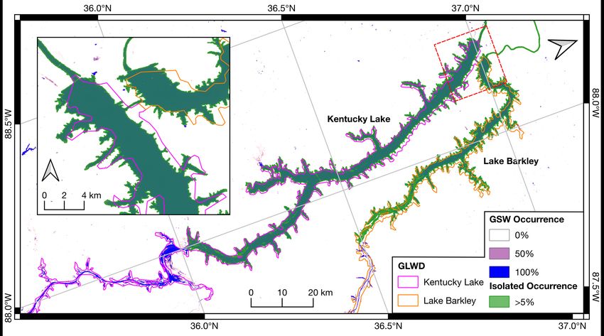
Remote Sens. 2020, 12, 3320                                                                         2 of 19

especially in remote areas [4]. Surface volume changes can be measured by satellites with two different
approaches: whereas gravity missions such as the Gravity Recovery and Climate Experiment (GRACE)
and its successor GRACE-FO observe total water storage changes with spatial resolutions of some
hundred kilometers [5], a combination of satellite altimetry and optical imagery can be used to directly
estimate surface water volume changes [6–8].
      Pre-processed remote sensing data for hydrological applications are disseminated by different
institutions. One platform is the Database for Hydrological Time Series of Inland Waters (DAHITI),
which is available at http://dahiti.dgfi.tum.de. DAHITI provides a variety of hydrological information
on lakes, reservoirs, rivers and wetlands derived from satellite data. The most important products
are water levels from satellite altimetry and water surface areas from satellite imagery. Moreover,
water occurrence masks are available for download. Currently, information on more than 2800 targets
is provided.
      Surface water masks derived from remote sensing data are valuable for many applications,
including flood plain monitoring and water resource studies. Moreover, they are commonly used in
satellite altimetry applications to define target locations and to remove measurements contaminated
by land. For that purpose, constant land-water-masks are usually used; e.g., the Global Lakes and
Wetlands Database (GLWD) mask [9] or the water mask MOD44W [10]. In recent years, dynamic masks
have also become common, especially for river applications. Different classification techniques have
been developed; e.g., techniques based on optical data from Landsat missions [11] or a combination
of optical and SAR missions [12]. Elmi et al. [13] developed an algorithm based on Moderate
Resolution Imaging Spectroradiometer (MODIS) data and provided an overview of other existing
methods. In addition to satellite imagery, other remote sensing techniques can also be used to extract
surface water information; for example, passive microwave land surface emissivities or scatterometer
responses [14] or altimeter radar echoes for water detection based on waveform classification [15].
      In contrast to GRACE and satellite imagery, due to its measurement principle, satellite altimetry
only delivers data along the satellites’ ground tracks; i.e., so-called along-track data directly beneath
the satellites. Depending on the active missions and their orbit configurations, some lakes are missed
for which no height information can be derived. The focus of this study is to investigate the capability
of different satellite altimetry configurations to measure basin-wide lake storage changes. As a study
case, the Mississippi basin in North America is used. In order to allow for a comprehensive inventory
of lakes and reservoirs covered by different satellite altimetry missions, an automatic tool for lake
detection has been developed as part of the study. Model storage information from WGHM is used to
assess the percentage of water volume changes missed due to the current insufficient data coverage of
satellite altimetry as well as the improvements expected from the upcoming new Surface Water and
Ocean Topography (SWOT) mission [16].
      The paper is structured as follows: Section 2 describes the study area and the used input data sets.
Afterwards, Section 3 introduces the used methods before Section 4 presents the results of the study,
followed by a discussion in Section 5 and some concluding remarks in Section 6.

2. Study Area and Input Data

2.1. Mississippi River Basin
     In this work, the Mississippi River Basin (MRB) is used as a case study area. Covering an area of
about 3,000,000 km2 , the MRB is the largest basin in North America and encompasses about 40% of the
area of the United States. Moreover, it is the third largest basin in the world after the Amazon and
Congo [17]. It is a region that is densely populated. In 1982, 18 million people relied on the Mississippi
for their water supply [18]. This has resulted in intense anthropogenic water use, due to which many
large reservoirs have been built up. The Mississippi, with its tributary the Missouri, is the longest
(about 3730 km) and largest (about 16,800 m3 /s) river in North America.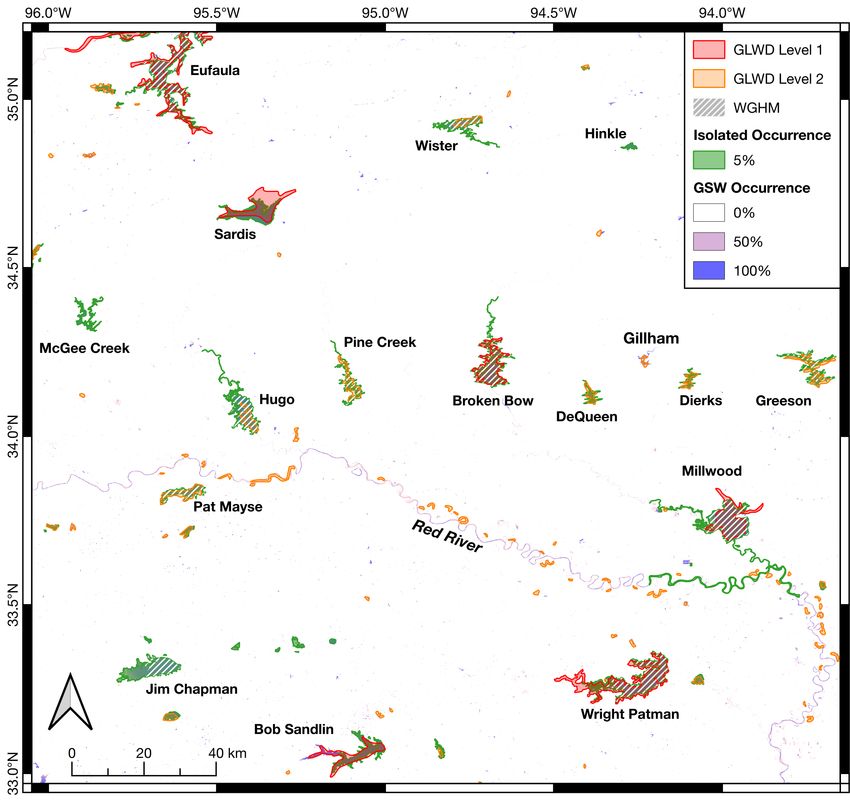
Remote Sens. 2020, 12, 3320 3 of 19
According to the WaterGAP hydrology model (see Section 2.5), a total of 127 lakes and reservoirs
are located in the MRB, from which only nine are defined as lakes and one as a regulated lake. All others
are reservoirs. Total water volume variations (defined as the sum of the differences between minimal
and maximal volume over the period 2003 to 2016) of 180 km3 and a surface area of 14,918 km2 are
documented for all water bodies (without rivers). The surface area varies between 3 and 1127 km2 and
the storage changes up to 18 km3 . According to the Global Reservoir and Dam Database (GRanD) [19],
a total water volume of about 250 km3 is stored in the reservoirs of the MRB. The entire study area is
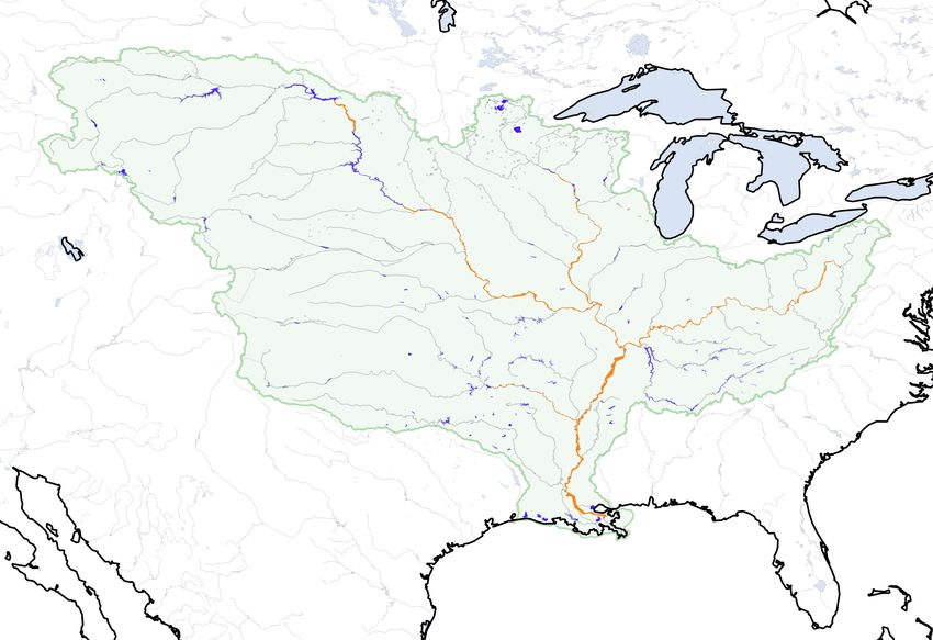
shown in Figure 1
Figure 1. The Mississippi River Basin: Lakes and reservoirs that are implemented in WaterGAP are
shown in blue, major rivers as grey lines. Orange: River sections that were removed manually (see
Section 3.3).
2.2. Satellite Altimetry Data
Satellite altimetry determines the distance between the satellite and the Earth’s surface in the
nadir direction by measuring the travel time of a microwave signal emitted by an instrument on
board of the satellite and reflected by the water surface on the ground. When the satellite’s height is
known, the surface elevation can be easily derived by subtracting both quantities. More details on the
measurement technology can be found in Chelton et al. [20], for example. Due to this measurement
geometry, satellite altimetry provides measurements along dedicated profiles—i.e., tracks—with a
high along-track resolution (depending on sensor and datasets between about 300 m and 7 km).
The cross-track resolution strongly depends on the satellite’s orbit configuration. Most altimetry
missions use repeat orbits and cover the same location on the Earth every 10 to 35 days. The higher the
temporal resolution, the lower the spatial cross-track resolution. By combining different missions in a
multi-mission approach, the temporal as well as the spatial resolution of the system can be significantly
improved. In this study, six different orbits are exploited, which are used by more than 10 different
satellites. These are described in more detail in the following. Table 1 summarizes the orbit parameters
for all of these altimetry missions.Remote Sens. 2020, 12, 3320 4 of 19
The lifetime of satellite missions is limited to a few years. In order to ensure the continuous and
consistent monitoring of the Earth’s surface, successor missions follow the original missions on the
same orbit. Important examples of this are the NASA/CNES missions TOPEX/Poseidon, Jason-1,
Jason-2 and Jason-3, which will soon be continued by Sentinel-6. All of these missions use the same
nominal orbit with a repeat cycle of about 10 days and a track separation at the equator of about
315 km.
The second long-term orbit is occupied by ERS-1, ERS-2 and Envisat. These ESA missions are
followed by the ISRO/CNES mission Saral that uses the same orbit but a different altimeter instrument
operating in the Ka-band; in contrast, all other missions emit Ku-band signals. This orbit is defined as
a 35-day repeat orbit with an 80 km track separation. Saral was launched in 2013, about three years
after Envisat left its nominal orbit. During this data gap between Envisat and Saral, no measurements
for this orbit were acquired.
The Copernicus mission Sentinel-3 consists of two satellites: Sentinel-3A and Sentinel-3B. Both
have the same orbit parameters but fly interleaved with each other with a 27-day repeat cycle, meaning
that they complement each other in spatial resolution. The Sentinel-3 constellation has a ground track
separation at the equator of 52 km.
In addition to these short-repeat missions, two missions are used within this study that fly on
long or non-repeat orbits. Cryosat-2 has a 369-day repeat. This results in a dense ground track pattern
but with a sparse temporal resolution at dedicated locations. However, due to its sub-cycle of about
30 days, larger lakes can be monitored with a monthly resolution.
Saral originally used the Envisat orbit. However, due to problems with the satellite, since 2016, the
orbit is no longer maintained on its nominal track but is in a drifting configuration without a regular
pattern over the long-term in the ground track. This results in irregular spatial–temporal sampling
on the ground but can help with monitoring lakes on a global scale, especially when this mission is
combined with other altimetry missions. This part of the missions is named Saral-DP (drifting phase).
Table 1. Orbit configuration of satellite altimetry missions used in this study.
Orbit Missions Period Heigth Repeat Cycle Track Dist.
[km] [days] at Equator [km]
Jason TOPEX, Jason-1/2/3 1992-today 1336 9.9 315
Envisat ERS-1/2, Envisat, Saral 1991–2010/2013–2016 800 35 80
Sentinel-3A Sentinel-3A 2016-today 815 27 104
Sentinel-3B Sentinel-3B 2018-today 815 27 104
Cryosat-2 Cryosat-2 2010-today 717 369 8
Saral-DP Saral-DP 2016-today changing drifting irregular
2.3. Water Occurrence Masks
Water occurrence or probability masks are available from different sources. In this study, we use
the Global Surface Water dataset (GSW) published by Pekel et al. [21], as this has a global coverage
and a high spatial resolution of about 30 m. It has been derived based on about three million Landsat
satellite images taken between 1984 and 2015. For each pixel, the water probability given in percentages
is provided, where a value of 50% might indicate either a permanent water occurrence in half of the
pixels for all 32 years of data or a full water pixel for half of the time period. These values can be used to
extract water masks for predefined water probability values; e.g., to derive lake shapes for permanent
water bodies in dry seasons (with a threshold of 100%) or for areas that are temporarily flooded (with
a threshold < 50%). More information on the methods used to convert GSW to land-water masks is
provided in Section 3.1.
2.4. Global Lakes and Wetlands Database
For comparison, information provided by the Global Lakes and Wetlands Database (GLWD) [9]
is used in this study; namely, shorelines and surface areas of Level 1 and Level 2. Level 1 providesRemote Sens. 2020, 12, 3320 5 of 19
metadata for the largest lakes (with a surface area larger than 50 km2 ) and reservoirs (storage capacity
larger than 0.5 km3 ) worldwide. Level 2 contains additional smaller lakes with surface areas larger
than 0.1 km2 . For the MRB, the database provides 120 level 1 lakes and 4527 lakes of level 2, with a
total area of 33,687.66 km2 (19,041.73 km2 for level 1 and 14,645.83 km2 for level 2). GLWD is used for
comparison, since it is the most commonly used and freely accessible global dataset available today.
2.5. Water Volumes from WaterGAP
In order to analyze the surface water volume that can be monitored by satellite altimetry in the
MRB, the WaterGap Global Hydrology Model WGHM [2] is used. The model simulates water resources
with a focus on anthropogenic inventions due to human water use and man-made reservoirs [22].
WGHM uses a spatial resolution of 0.5◦ , and the temporal resolution of the model output used within
this paper is monthly. A comprehensive description of the current model—version 2.2d—used within
the context of this study is given by Müller Schmied et al. [22].
Water bodies are represented within the model as area fractions of the 0.5◦ grid cells. The GLWD
(Section 2.4) and the GRanD database [19,23] are used for the definition of water bodies within the
model. Each water body is defined as lake, regulated lake, reservoir or wetland. Furthermore, the
model distinguishes between local and global water bodies: lakes are implemented as global if their
area is larger than 100 km2 , and for regulated lakes and reservoirs, a threshold of 0.5 km3 storage
capacity or 100 km2 minimum area is applied [22]. In this study, global lakes, regulated lakes and
reservoirs are used (no local water bodies). As bathymetry and the initial volume of the water bodies
are unknown to the model, the WGHM water volumes for global water bodies are treated as anomalies.
For reservoirs and regulated lakes, the maximum storage capacity is applied as an upper threshold [22].
The commissioning year (GranD database) is used to start filling reservoirs and, if applicable, to change
the type of the water body from a lake to regulated lake [22].
3. Method: Automated Target Detection
The identification of lakes and reservoirs that can be monitored by satellite altimetry needs
information on the satellite’s ground track on the one hand and knowledge of the location and extent
of water bodies on the other hand. The latter can be taken from existing data sets such as GLWD or
Hydrosheds [24]. These provide constant water body shapes without considering any time-dependent
variation due to seasonal or long-term changes. Alternatively, satellite images can be used to derive
time-variable land–water or water occurrence masks, as are available from optical Landsat and
Sentinel-2 images [25], for example. Those data have already been used to derive inventories of global
lakes; e.g., by Verpoorter et al. [26] and Feng et al. [27].
In this study, the Global Surface Water dataset (GSW) from Pekel et al. [21] (see Section 2.3) is used
as input data. However, the developed procedure is able to handle any arbitrary water occurrence
mask in raster format; e.g., DAHITI occurrence masks [8]. Furthermore, minimal manual interaction
is required, and it is therefore suitable for large amounts of data—e.g., the MRB—and can be rerun
easily if an updated version of the input water occurrence masks is available. The possibility to set
parameters according to particular needs enables the application of the procedure in variable scenarios;
e.g., studies of water bodies with permanent water coverage or those that are only seasonally flooded.
The main idea of this work is to identify connected water areas and to define the water body
outlines based on a pre-defined threshold of water probability, which can later be transferred to
other probability levels. The assumption is that all areas of one water body have the same height.
Thus, the approach is suitable for lakes and reservoirs but not for rivers. Due to the slope of the
river, each satellite’s overflight defines a new target (i.e., a virtual station) at the crossing between the
satellite’s ground track and the river. For that reason, the developed approach is only applicable to
lakes and reservoirs.
The developed algorithm consists of two major steps. First, individual water bodies are identified
by applying several morphological operations that are widely used in image processing [28]. This isRemote Sens. 2020, 12, 3320 6 of 19
described in more detail in Section 3.1. In the second step (described in Section 3.2), isolated occurrence
masks based on the GSW data are processed for each identified water body to analyze their coverage by
satellite altimetry data at different water occurrence thresholds. A flowchart illustrating the developed
methodology can be found in the Appendix A (Figure A1).
3.1. Morphological Operations
The basis for deriving the water masks is the GSW dataset introduced in Section 2.3. This is
transformed into one binary land–water mask by defining a threshold value of 50%. This value will
ensure the extraction of a mean surface area for permanent lakes/reservoirs with seasonal changing
areas. Moreover, targets that are only temporally flooded will also be detected as well as reservoirs,
which are created within the observation period of GSW; i.e., after 1984 but before about 2000. Later,
masks for different water occurrences are derived (Section 3.2) and their impact is studied in Section 5.2.
The binary input mask is subject to three different morphological operations from image
processing: erosion, dilation and closing [28]. To define the effect of the operators on the image,
quadratic kernels are used as structuring elements. First, an erosion is performed on the binary input
mask. This is done to remove small-scale water bodies such as rivers, ponds and very small lakes. For
these small-scale waters, it is difficult to infer satellite altimetry water level time series with sufficient
data quality because of the influence of land (see Section 5.4). On the other hand, their removal speeds
up the processing significantly. The kernel diameter is set to 21 pixels (approximately 630 m, depending
on the geographic latitude), leading to the removal of all water bodies that are consistently narrower.
The effect of this step is shown in Figure 2: Figure 2a displays the original binary mask and Figure 2b
shows the resulting mask after the erosion was performed. Subsequently, the inverse operation, called
dilation, is performed with a kernel size of approximately 4830 m (161 pixels), indicated by the grey
area in Figure 2c. In order to preserve the original water body outlines, the result is overlain with the
initial binary mask. Only pixels that are marked as water in both masks will be regarded as water
in the resulting land water mask; i.e., the intersection between both is taken (called conjunction in
Figure A1). This intersection is marked in white in Figure 2c. In the last step, a closing operation with
a kernel size of about 390 m (13 pixel) is applied. This operation removes small islands and bridges.
This allows two parts of a water body that are separated by bridges, for example, to be united (see
Figure 2d.)
Figure 2. Visualization of the morphological operations used in the automated target detection:
(a) initial land–water mask, (b) after erosion, (c) after dilation, (d) final land–water mask.
3.2. Lake Shapes for Different Water Occurrences
The target detection is performed based on a fixed water occurrence threshold of 50% (see
Section 3.1). In order to conduct overflight statistics (Section 3.4) and to study the impact of different
thresholds (Section 5.2), isolated water occurrence masks are required. Performing the morphological
operations repeatedly for different thresholds (i.e., repeating the full image processing procedure)
incurs great time and computational costs. Instead, the binary land–water mask (output of Section 3.1)Remote Sens. 2020, 12, 3320 7 of 19
covering the entire MRB is vectorized to reduce the computational time necessary to process the
raster data. The result is one polygon feature per isolated water body. In order to extract the isolated
water occurrence, the water occurrence mask is clipped to the bounding box of each feature with a
buffer of 0.15◦ , which is required because narrow ends of dendritic reservoirs may have been lost
due to the morphological operations. The clipped water occurrence mask is again transformed to a
binary land–water mask, but this time with an occurrence threshold of 5%. Afterwards, each binary
mask is labeled (i.e., connected pixels are marked with a consistent integer), and the label of the
corresponding water body is identified using the pole of inaccessibility (POI) of the respective polygon;
i.e., the spot furthest from the lakeshore [29]. The POI is very likely to be located above a pixel with a
high occurrence. We isolate the water occurrence of each target using the respectively labeled pixels as
a mask.
Due to the morphological operations, contiguous water bodies may be separated, especially at
the shore of dendritic reservoirs. This results in duplicate isolated water occurrence masks. In order to
detect these duplicates, intersections between the shorelines of all isolated masks are searched, and the
smaller intersecting masks are removed.
Based on the isolated water occurrence masks, the water extent and surface area of each target
can be extracted for different occurrence thresholds. In this study, we used thresholds of 5%, 25%, 50%,
75% and 95% in order to calculate the satellite altimetry overflight statistics (Section 3.4).
3.3. Removal of Rivers and Coastal Data
The aim of the automated target detection is to identify lakes and reservoirs for which a constant
water level per observation epoch is assumed. Due to the slope of rivers, water level time series
can be derived only for particular river sections and not for entire rivers. For the same reason, most
satellite altimetry time series for river targets are based on a single mission, except for the rare cases of
crossing tracks above a river. In consequence, rivers cannot be processed in the same way as lakes and
reservoirs, for which the water level is assumed to be independent of the topography. Therefore, rivers
are not part of this study and should not form part of the detected water targets.
Since rivers are part of GSW—and also of any other water occurrence product based on satellite
images—they have to be excluded from the water mask within the process of target detection. This is
easy for smaller rivers, which are removed by the erosional step. However, some rivers might be wider
than some narrow reservoirs as a result of river impoundments. Therefore, it is not possible to define a
kernel size that removes all rivers but preserves all lakes and reservoirs at the same time. Thus, major
rivers are removed manually from the binary dataset (resulting from Section 3.1) by setting all water
pixels within the river polygons to land. All rivers sections removed manually from the binary dataset
are indicated in orange in Figure 1.
However, there are still river segments in the isolated water occurrence masks; this is caused
by small water bodies near to and partly connected to a river. These masks have to be manually
identified by visual inspection and removed from the dataset. The same holds for large, connected
water systems at the coast, which cannot clearly be defined as a single water body or distinguished
from the ocean. The primary reason for the manual interaction is to provide reliable statistics for this
paper. Significantly less interaction is required for the target detection itself.
3.4. Connection to Satellite Altimetry Data
In order to decide whether a lake is mapped by one of the satellite altimetry missions, their
ground tracks have to be analyzed. For this purpose, the individual measurement locations instead
of the nominal ground tracks are used. Thus, for each individual altimetry observation, we verify
whether it is taken above one of the detected water bodies. With this strategy, missions on non-repeat
orbits such as Saral-DP can also be handled.
A water body is regarded as being monitored by a mission if at least four valid overflights per
year (in average) are detected. This ensures the monitoring of the lake’s seasonality even for missionsRemote Sens. 2020, 12, 3320 8 of 19
on long or non-repeat orbits (Cryosat-2 and Saral-DP). For the short-repeat missions (Envisat, Jason
and Sentinel-3A/B), which cover the same location every 10 to 35 days, the temporal resolution will be
always better; i.e., at least once per month.
4. Results
The automated target detection approach described in Section 3 with a water occurrence threshold
of 50% identified 4535 water bodies with surface areas of 0.1 to 1291.04 km2 and a total sum of
29,100.72 km2 . The mean area is 6.4 km2 . In total, 2061 lakes/reservoirs were found that are larger
than 1 km2 , 429 that are larger than 10 km2 and 45 that are larger than 100 km2 . While the number
of detected water bodies was very close to the number given in GLWD (Level 1 and Level 2), which
is 4647, the total area is underestimated by almost 4600 km2 (the area from GLWD is 33,688 km2 ).
This changes with the use of different water occurrence incidences (see Section 3.2 for details). The
number of water bodies, as well as their surface area, increases if no limitation of water occurrence
is used (>5%). In this case, 5708 lakes larger than 0.1 km2 are identified with a total surface area of
35,397.54 km2 . Figure 3 shows the numbers for different thresholds of water occurrence probabilities.
The blue line represents the results for all water bodies larger than 0.1 km2 . For the red and orange
lines, larger lake size limits of 1 and 10 km2 are applied. The number and size of detected lakes larger
than 10 km2 for higher water occurrences correspond well with those from GLWD Level 1 and WGHM.
Figure 3. Number (left) and total area (right) of detected lakes in the Mississippi River Basin (MRB)
depending on the adopted water occurrence probabilities for three different minimum lake sizes (blue:Remote Sens. 2020, 12, 3320 9 of 19
The statistics presented here are based on a water occurrence of 50% and all 4535 water bodies
larger than 0.1 km2 (blue dot with black edge in Figure 3). In total, 3437 of those targets (75.7%)
have not been covered by any of the current and past missions under investigation. Since these are
mostly smaller lakes or reservoirs, the percentage of not covered water area is only 17.5% (5108 out
of 29,101 km2 ). Depending on the ground tracks of the different missions, they cover a different
number of targets. The best scenario is the current configuration of Jason-3, Sentinel-3A/B, Cryosat
and Saral-DP, which captures about 19% of the water bodies and 79% of the surface areas. With
respect to past altimetry configurations (i.e., Jason-2 and Envisat), this is a significant improvement.
All numbers are summarized in Table 2.
Table 2. Number and area of lakes/reservoirs larger than 0.1 km2 covered by different altimetry
constellations. The values in parentheses are the percentages of the total number and total
area, respectively.
Scenario Number of Targets Area of Targets in km2 Mean Size of Targets in km2
Jason only 212 (4.7%) 9125 (31.3%) 43.0
Sentinel-3A/B 704 (15.5%) 20893 (71.7%) 29.7
Past configuration 612 (13.5%) 18090 (62.0%) 29.6
Current configuration 853 (18.8%) 23110 (79.3%) 27.1
As expected, most of the larger lakes are captured by the altimetry missions. The smaller a
lake, the higher the probability that it is missed by the satellites. Figure 4 shows the percentage
of missed water bodies for the four different mission scenarios depending on the size of the lakes.
With the current configuration, all lakes larger than 50 km2 and almost 20% of the lakes larger than
10 km2 are captured. This is a significant improvement with respect to the past configuration of
Jason and Envisat, which missed almost 40% of all water bodies larger than 20 km2 . However, even
today, about 67% of all water bodies larger than 1 km2 are missed in the MRB. This number will only
be improved significantly when a wide-swath altimetry mission such as SWOT—planned for 2021
(see Section 5.5)—will become active. When only using Jason, more than 60% of lakes larger than
100 km2 cannot be monitored, whereas the Sentinel-3 configuration alone performs better than the
past configuration of Jason and Envisat.
Figure 4. Percentage of missed lakes/reservoirs for different altimetry configurations depending on
minimal target size (from 1 to 100 km2 ) based on a water occurrence threshold of 50%.
4.2. Surface Water Storage
For the monitoring of surface freshwater resources, water storage and its changes are more
important than the number of lakes or their surface area. However, optical images, as used in Section 3,Remote Sens. 2020, 12, 3320 10 of 19
are not able to provide any information on water volume or lake bathymetry. First approaches
exist to derive storage changes and lake bathymetry from remote sensing techniques (for example,
Schwatke et al. [8] and Li et al. [30]), even on a global scale [7],[31]. However, since these approaches
also rely on satellite altimetry, they are not able to provide information for all water bodies. The most
comprehensive databases for water volume are still global hydrological models, even if, in these
records, the very small water bodies are missing.
WGHM provides 127 lakes and reservoirs in the MRB with areas between 2.9 and 1126.8 km2 (total
sum of 14,671.2 km2 ) and water volume variations up to 18.2 km3 . From these targets, three reservoirs
are not detected by the automated target detection method developed in this study. They have a total
area of about 20 km2 (2.9, 12.4 and 4.8 km2 ) and are all very narrow. In total, 124 of all detected targets
are available in WGHM (2.7%), representing about 50% of the total detected surface area.
From the 127 WGHM targets, 116 can be mapped by one of the altimetry missions handled in this
study; however, not at the same time. Eleven are not covered at all. In the past, with a combination
of satellites from the Jason and Envisat family (past configuration), about 76% of the water volume
variations issued by WGHM were detectable. In comparison, the current configuration of Jason,
Sentinel-3, Cryosat-2 and Saral-DP meets the requirement of monitoring 98% of the water volume of
lakes and reservoirs in the MRB (since 2018). When using only Jason, this number is much smaller,
at about 50%. All numbers can be found in Table 3.
Table 3. Water storage changes from WGHM that are mapped by different altimetry constellations.
The values in parentheses are the percentages of the total number and total volume variations from
WGHM, respectively.
Scenario Number of Targets Water Volume Variation Mean Variations Mean Size
in km3 in km3 in km2
Jason only 29 (22.8%) 90.6 (50.4%) 3.13 224.2
Sentinel-3A/B 97 (76.4%) 161.9 (90.1%) 1.67 129.7
Past configuration 71 (55.9%) 137.1 (76.3%) 1.93 158.5
Current configuration 116 (91.3%) 176.5 (98.1%) 1.52 123.9
Although WGHM represents only about half of the available water surface area in the MRB
(14,671 of 29,101 km2 defined by the automated target detection), about 300 km2 (2% of the WGHM
total area) still cannot be mapped by satellite altimetry due to the orbit configuration of the missions.
The averaged surface area of WGHM targets is 116 km2 and the mean size of mapped water bodies is
124 km2 . The percentage of missed water volume changes is in the same order of magnitude: about 2%
of WGHM storage changes cannot be monitored by current satellite altimetry. Thus, it is reasonable
to say that the current altimetry configuration is able to provide almost the same information to
that available from global hydrological models. However, the temporal resolution differs: while
WGHM provides monthly values, the altimetry resolution can yield values from a few days to 10
or 35 days, or even fewer, depending on the missions involved (see Sections 2.2 and 5.4). However,
concerning long-term storage changes, approximately 25% are missed by the satellites, even reaching
50% when only Jason missions are used. These numbers improve when only considering larger lakes
(see Figure 5). With the current configuration, storage changes of all lakes larger than 80 km2 can be
monitored, whereas Jason still misses about 15 km3 for lakes larger than 200 km2 .Remote Sens. 2020, 12, 3320 11 of 19
Figure 5. Missed WGHM storage changes as a function of minimal lake sizes for different
altimetry configurations.
It should be noted that all numbers presented here are based on information about the satellites’
orbit configurations; i.e., whether a lake is crossed by any of the satellites’ tracks. Additional lakes will
be missed when no reliable height information can be determined, which is especially conceivable for
small lakes with a steep surrounding topography (see Section 5.4 for more details).
5. Discussion
5.1. Assessment of Automated Target Detection
With 5708 targets, about 1000 more water bodies were identified in this study (applying an
occurrence threshold of 5%) compared to the 4647 found with GLWD Level 1 and 2 data (see Figure 3).
However, the datasets differ not only by the additional water bodies identified in this study, but also
by some missing targets which are contained in GLWD.
As example, Figure 6 shows an area along the Red River at the border between Arkansas and
Oklahoma. Several water bodies identified in this study are not part of GLWD Level 1 or 2, such as the
lakes Jim Chapman, McGee Creek, Hinkle and some smaller targets east of the Jim Chapman Lake;
however, these are contained in WGHM. However, some water bodies are not identified, even though
they are available in GLWD; this could be because they are too small, as with Lake Gillham—i.e.,
consistently narrower than 630 m—and removed by the morphological operations (Section 3.1),
or because they are connected to a river (by water occurrence pixels above 5%) and removed manually
(Section 3.3) as they could not be distinguished from the river. Furthermore, the different sizes of some
lakes are noteworthy. For example, Lake Hugo and Lake Wister are both much smaller in GLWD than
in this study.
Sometimes, the separation between a lake and river is not clear, since the method is not able to
distinguish between a narrow reservoir and a wide river. In these cases, part of the river is identified
as a lake area (e.g.,s Lake Broken Bow and Millwood Lake). In rare cases, such targets can cause an
error in the overflight statistics when the satellite track crosses the connected remaining river but not
the water body that is the actual target. On a basin-wide average, the water surface area differs by
1710 km2 (about 5%) with respect to GLWD (see Figure 3).Remote Sens. 2020, 12, 3320 12 of 19
Figure 6. Isolated occurrence of detected targets (green), GLWD Level 1 (red) and 2 (orange) and
WGHM data (white hatched) surrounding the Red River at the border between Arkansas and Oklahoma.
Additionally, the GSW water occurrence is shown as background.
Other challenges arise due to the definition of targets. For example, the lakes Barkley and
Kentucky, as shown in Figure 7, are actually one water body connected by the unregulated Barkley
Canal. While they are automatically identified as one target in this study, as indicated by the green
polygon in Figure 7, they are treated separately in the GLWD dataset. Another challenge in terms of
definition is the extent of a reservoir upstream of the respective dam. There is no clear border between
the river and the reservoir, and thus the size of both lakes is larger in GLWD compared to this study.
The comparison also shows that the water body outline identified in this study is more detailed and
accurate than the GLWD data.Remote Sens. 2020, 12, 3320 13 of 19
Figure 7. Lake Barkley and Kentucky, separated in the GLWD data (purple and orange) and merged
in the isolated results of this study (green). Additionally, the GSW water occurrence is shown as a
background. The inset shows the area close to the dams and the Barkley Canal connecting both lakes.
Challenging conditions are also found in the coastal wetlands, where some possible targets
cannot be distinguished from the ocean or connected water bodies. In rare cases, targets are removed
by the erosional step or the POI is not within the area of high occurrence of a water body (e.g., an
island), resulting in incorrect labeling and isolation. Both errors occur predominantly in narrow
dendritic reservoirs.
By changing the pixel sizes of the morphological operation, the method can be optimized to find
more or less narrow structures. However, automated processes will never be able to distinguish a
bridge over a reservoir (which should be removed from the images) from an equally sized dam of
a reservoir (which should be left in the image). The applied parameters have proved to be a good
compromise to detect most of the relevant water bodies without identifying too many unwanted
targets. However, since no ground truth is available, fine-tuning based on statistical validation for the
entire MRB is not possible.
5.2. Impact of Different Water Occurrences
The overflight statistics presented in Section 4.1 change as the lake shapes vary: at a high water
level, a lake will cover a larger area and will have a higher probability of being crossed by an altimeter
track. In this study, occurrence masks are used to extract lake shapes for different water levels
(Section 3.2). When increasing the water occurrence threshold from 50% to 95% the number of detected
lakes decreases (see Figure 3) since only permanent water is counted. At the same time, the mean size
of the detected lakes increases (from 6.4 to 11.4 km2 ) as more larger lakes have permanent flooded
parts. Consequently, fewer lakes are missed by the altimetry missions when the occurrence threshold
is increased. Instead, a lower occurrence threshold means that more lakes cannot be monitored since
they are no longer crossed by a satellite’s track. Figure 8 illustrates the percentage of missed lakes
for different water occurrences for lakes larger than 0.1 km2 and lakes larger than 10 km2 . Whereas
nearly 90% of the smaller non-permanent lakes are missed by the past altimetry configuration at
the 5% occurrence threshold (and 85% by the current threshold), these numbers decrease to 75%
(and 63%) at a 95% occurrence threshold. When limiting the analysis to lakes larger than 10 km2 ,
the number of missed lakes is smaller for all occurrence thresholds but shows the same behavior.Remote Sens. 2020, 12, 3320 14 of 19
The current configuration of altimeter satellites is able to monitor about 84% of these lakes when taking
all occurrences into account.
Figure 8. Percentage of missed lakes/reservoirs for different altimetry configurations and different
water occurrences. Left: all water bodies larger than 0.1 km2 ; right: water bodies larger than 10 km2 .
It may be worth mentioning that, with decreasing water occurrence, not only are altimetry
observations less frequent but also of lower quality due to the expected increased land contamination
(see Section 5.4).
5.3. Impact of Neglecting Rivers and Smaller Lakes that Are Not Available in WGHM
When investigating the percentage of monitored surface water storage in Section 4.2, smaller
lakes that are not available in WGHM as well as water available in rivers have been neglected.
Rivers only store 0.006% of global freshwater. Most of the world’s freshwater is stored in icecaps
and glaciers and as groundwater (nearly 99%) [32]. From the remaining 1.2% of global freshwater,
river water storage comprises less than 0.5%, whereas lakes store nearly 21% [1]. The small percentage
of river water justifies the focus on lakes and reservoirs. Even if the Mississippi contains more water
than most other rivers, the entire MRB is so large that global conditions can be assumed.
The impact of neglecting lakes smaller than 0.1 km2 can be assessed using the analyses performed
by Downing et al. [33] based on statistical extrapolations. They estimated the number of lakes with
areas from 0.001 to 0.1 km2 to be 99% of all lakes and to cover about 30% of the overall global lake
area. When assuming that this relation can be transferred to the MRB, 30% of the total lake area
would have been missed as lakes smaller than 0.1 km2 were neglected: i.e., 12,472 km2 . The lower
percentage published by Verpoorter et al. [26] (about 4.8% of the area of all lakes, leading to around
2000 km2 being neglecged) based on remote sensing data is at least partly due to the spatial resolution
and detection limit of the used satellite imagery. However, this documents the continuing lack of
knowledge regarding the number and area of small lakes on Earth well. Current remote sensing
instruments are not able to shed light on this since the spatial resolution of satellite techniques is
limited. Moreover, the lake abundance is changing rapidly in some regions [26], and each study can
only present a snapshot of the respective situation.
With respect to lake volume changes, the relation presented by Biancamaria et al. [34] suggests
that 20% of global storage changes are due to lakes smaller than 0.1 km2 . Due to the resolution limits
of satellite altimetry (including SWOT), these percentages cannot be monitored from space in the
foreseeable future. Assuming that WGHM includes all water bodies with areas larger about 3 km2 ,
slightly more than 50% of storage changes should be captured. Consequently, nearly 50% (aboutRemote Sens. 2020, 12, 3320 15 of 19
180 km3 ) of all lakes are not included in WGHM. If one aims at smaller lakes, regional hydrological
models must be used.
5.4. Limitations of Satellite Altimetry Height Estimation
It is important to keep in mind that even if a lake or reservoir is located beneath a ground track of
a satellite altimetry mission, it is not always possible to derive valid height information. The ability to
reliably generate water level time series strongly depends on the size of a water body, especially on
the length of the satellite’s track over the water; however, this is not the only influence. The quality of
the measurements are also affected by the surrounding topography, the sensor type on board of the
satellite and other factors. Thus, no generally applicable size limit can be defined. While Biancamaria
et al. [34] proposed a limit of 100 km2 referencing work from 2002 and 2006, Baup et al. [35] showed
results for a 0.52 km2 small lake in France and Biancamaria et al. [36] used satellite altimetry to monitor
the River Garonne, which is only 200 m wide.
For the MRB, using the DAHITI processing approach [37], reliable long-term water level time
series for 54 lakes and reservoirs can be derived, from which 41 targets can be seen to be part of WGHM.
This is about 58% of the WGHM targets mapped by the past altimetry configuration. The minimal size
of the observed WGHM lakes is 10 km2 . The smallest lake for which water level time series can be
derived and which is not part of WGHM is 3.4 km2 (with a 50% occurrence threshold). For the WGHM
targets that are missing in DAHITI, no accurate long-term water level time series can be derived. This is
mostly due to the shape of the lakes (very narrow) or due to satellite tracks being close to the lakes’
shorelines. However, it is important to keep in mind that these numbers are not easily transferable to
other basins, since the local characteristics strongly influence the quality of altimetry-derived water
level time series.
Another point worthy of mention here is the temporal resolution of the altimetry-derived time
series. As already indicated in Section 2.2, this strongly depends on the repeat cycle of the satellite as
well as on the number of tracks covering a lake or reservoir. In this study, a water body is counted as
monitored when at least four overflights per year are identified (see Section 3.4). Thus, time series with
temporal resolutions of three months up to a few days can be generated depending on the lakes’ size
and location. This ensures that seasonal variations are captured but will not guarantee the monitoring
of short-term extreme events, especially for smaller lakes.
5.5. Outlook for SWOT
The Surface Water and Ocean Topography (SWOT) mission is planned to be launched in 2021.
In addition to a classical nadir-looking Ku-band altimeter, the mission will carry a Ka-band radar
interferometer called KaRin. This instrument will provide water level height information in two 50 km
wide swaths with a 20 km nadir gap (which is partly covered by the nadir altimeter) [38]. The spatial
resolution within this 120 km wide area varies between 10 and 60 m with an along-track pixel size
of 2.5 m [38]. Consequently, SWOT will cover nearly all continental surfaces up to a latitude of ±78◦
without larger data gaps. The total gap area in this region is about 3.5% of the total land area [39],
which is mostly located close to the equator. For the MRB, which is located north of 25◦ N, no gaps
due to the orbit configuration will occur, and all water bodies will be covered at least once within
the 21 day repeat period. The temporal resolution strongly depends on the geographic latitude and
will differ between two and four times per 21 days within the MRB (unevenly distributed). This is
still not optimal and will not lead to all extreme events being caught. However, the combination with
observations from classical missions will further increase the temporal resolution of several time series.
Even if the requirement of SWOT is to monitor all lakes larger than 1 km2 [34], the mission aims
to measure the spatio-temporal variability of lakes and reservoirs larger than approximately 250 by
250 m or 0.06 km2 [40]. Thus, about two-thirds of global lake and reservoir storage variations can
be captured [39]. Moreover, SWOT can also provide information on the surface area of lakes andRemote Sens. 2020, 12, 3320 16 of 19
reservoirs; thus, it performs its own target detection. This also enables the determination of improved
storage information from the simultaneously measured area and height information.
Thus, the future prospects are excellent thanks to SWOT. However, long-term studies still
dependent on the older, incomplete data from classical missions. Moreover, careful calibration and
combination concepts are necessary in order to ensure a consistent linkage of SWOT with historical
datasets and with data from current nadir altimeters.
6. Conclusions
Using the example of the Mississippi River Basin, this study shows the potential and limitations
of satellite altimetry in the monitoring of basin-wide surface water storage changes. Based on a newly
developed automated target detection method, the number and size of all lakes larger than about
0.1 km2 in the MRB can be determined. The merging of this information with past and current satellite
altimeter constellations reveals an overview of the possibilities of remote sensing technique to monitor
lake storage changes from space.
With the developed target detection approach, about 5700 lakes and reservoirs can be detected in
the MRB. This is in accordance with the information of GLWD, even if a larger total surface area is
documented. This number reduces significantly when only water bodies with permanent water are
taken into account.
The study reveals that in the MRB, with the current altimeter configuration consisting of Jason,
Sentinel-3, Cryosat-2, and Saral-DP, only about 20% of water bodies larger than 0.1 km2 can be captured
currently by satellite altimetry. This number increases to about 80% for lakes larger than 10 km2 , even
though reliable water level time series are not determinable for all of these. The main limitation is
the measurement technique, which requires the satellites to directly overpass the water bodies for
reliable measurements. When analyzing the larger water bodies available in the global hydrology
model WGHM, the situation improves: from these larger lakes, more than 90% are captured by satellite
altimetry, and 98% of the related storage changes can be monitored. However, for long-term studies
that rely on past altimeter configurations, the situation is significantly worse: until 2016, nearly 25% of
storage changes (i.e., more than 40 km3 ) are missed by the satellite tracks.
This study is limited to the MRB and not directly transferable to other basins with different lake
densities and characteristics. However, since the region is quite large, with significant variations in the
number of lakes per 106 km2 [33], transferability to a global scale might be valid.
Significant improvements are expected from the new SWOT mission, which will cover the entire
MRB without any data gap due to the orbit configuration of the mission. Moreover, smaller lakes will
be reliably measured due to the higher spatial resolution and increased height precision. However,
challenges will remain; in particular, the consistent combination of SWOT with classical altimetry data
and the deviation of volume changes without good knowledge of the lakes’ bathymetry. Besides that,
after 2021, the greatest limitation of satellite altimetry will be the temporal resolution of time series
and the risk of missing extreme short-periodic events.
Author Contributions: D.D. conceptualized the research work and wrote the major part of the manuscript;
L.E. developed the automated target detection method and prepared a draft version of the paper. L.E., C.S. and
D.S. performed the data processing. C.N. provided the lake volume changes from WGHM. C.S., D.S. and C.N.
contributed to the writing of the manuscript and helped with the discussion of the applied methods and results.
All authors have read and agreed to the published version of the manuscript.
Funding: This research was funded by the German Research Foundation DFG grant number DE 2174/10-1.
Acknowledgments: The authors would like to acknowledge the European Commission’s Joint Research Centre
for allowing access to the Global Surface Water Explorer GSWE (https://global-surface-water.appspot.com/).
The support of the German Research Foundation (DFG) within the framework of the Research Unit GlobalCDA
(FOR2630) is gratefully acknowledged. We thank four anonymous reviewers for their valuable comments that
helped to improve the manuscript.
Conflicts of Interest: The authors declare no conflict of interest.Remote Sens. 2020, 12, 3320 17 of 19
Appendix A. Flowchart of developed target detection method
Figure A1 illustrates all steps of the automated target detection method and their inter-connection.
The grey boxes indicate the sections of the work in which detailed information on the algorithms can
be found.
Figure A1. Flowchart of automated target detection, as described in Section 3.
References
1. Shiklomanov, I. World fresh water resources. In Water in Crisis: A Guide to the World’s Fresh Water Resources;
Gleick, P., Ed.; Oxford Universtity Press: Oxford, UK, 1993; pp. 13–23.
2. Müller Schmied, H.; Eisner, S.; Franz, D.; Wattenbach, M.; Portmann, F.T.; Flörke, M.; Döll, P. Sensitivity of
simulated global-scale freshwater fluxes and storages to input data, hydrological model structure, human
water use and calibration. Hydrol. Earth Syst. Sci. 2014, 18, 3511–3538. [CrossRef]
3. Döll, P.; Douville, H.; Güntner, A.; Müller Schmied, H.; Wada, Y. Modelling Freshwater Resources at the
Global Scale: Challenges and Prospects. Surv. Geophys. 2016, 37, 195–221. [CrossRef]
4. Alsdorf, D.E.; Rodríguez, E.; Lettenmaier, D.P. Measuring surface water from space. Rev. Geophys. 2007, 45.
[CrossRef]
5. Zaitchik, B.F.; Rodell, M.; Reichle, R.H. Assimilation of GRACE Terrestrial Water Storage Data into a Land
Surface Model: Results for the Mississippi River Basin. J. Hydrometeorol. 2008, 9, 535–548. [CrossRef]
6. Gao, H. Satellite remote sensing of large lakes and reservoirs: From elevation and area to storage.
WIREs Water 2015, 2, 147–157. [CrossRef]
7. Busker, T.; de Roo, A.; Gelati, E.; Schwatke, C.; Adamovic, M.; Bisselink, B.; Pekel, J.F.; Cottam, A. A global
lake and reservoir volume analysis using a surface water dataset and satellite altimetry. Hydrol. Earth
Syst. Sci. 2019, 23, 669–690. [CrossRef]
8. Schwatke, C.; Dettmering, D.; Seitz, F. Volume Variations of Small Inland Water Bodies from a Combination
of Satellite Altimetry and Optical Imagery. Remote Sens. 2020, 12, 1606. [CrossRef]
9. Lehner, B.; Döll, P. Development and validation of a global database of lakes, reservoirs and wetlands.
J. Hydrol. 2004, 296, 1–22. [CrossRef]Remote Sens. 2020, 12, 3320 18 of 19
10. Carroll, M.; DiMiceli, C.; Wooten, M.; Hubbard, A.; Sohlberg, R.; Townshend, J. MOD44W MODIS/Terra Land
Water Mask Derived from MODIS and SRTM L3 Global 250m SIN Grid V006 [Data set]; NASA Earth Observing
System Data and Information System Land Process Distributed Active Archive Centers: Sioux Falls, SD,
USA, 2017. [CrossRef]
11. Marshall, A.; Deng, X. Image Analysis for Altimetry Waveform Selection Over Heterogeneous Inland Waters.
IEEE Geosci. Remote Sens. Lett. 2016, 13, 1198–1202. [CrossRef]
12. Biswas, N.K.; Hossain, F.; Bonnema, M.; Okeowo, M.A.; Lee, H. An altimeter height extraction technique
for dynamically changing rivers of South and South-East Asia. Remote Sens. Environ. 2019, 221, 24–37.
[CrossRef]
13. Elmi, O.; Tourian, M.J.; Sneeuw, N. Dynamic River Masks from Multi-Temporal Satellite Imagery:
An Automatic Algorithm Using Graph Cuts Optimization. Remote Sens. 2016, 8, 1005. [CrossRef]
14. Prigent, C.; Papa, F.; Aires, F.; Rossow, W.B.; Matthews, E. Global inundation dynamics inferred from
multiple satellite observations, 1993–2000. J. Geophys. Res. 2007, 112, D12107. [CrossRef]
15. Dettmering, D.; Schwatke, C.; Boergens, E.; Seitz, F. Potential of ENVISAT Radar Altimetry for Water Level
Monitoring in the Pantanal Wetland. Remote Sens. 2016, 8, 596. [CrossRef]
16. Durand, M.; Fu, L.L.; Lettenmaier, D.P.; Alsdorf, D.E.; Rodriguez, E.; Esteban-Fernandez, D. The Surface
Water and Ocean Topography Mission: Observing Terrestrial Surface Water and Oceanic Submesoscale
Eddies. Proc. IEEE 2010, 98, 766–779. [CrossRef]
17. Niebling, W.; Baker, J.; Kasuri, L.; Katz, S.; Smet, K. Challenge and response in the Mississippi River Basin.
Water Policy 2014, 16, 87–116. [CrossRef]
18. Mississippi River Facts. Available online: https://www.nps.gov/miss/riverfacts.htm (accessed on
7 July 2020).
19. Lehner, B.; Liermann, C.R.; Revenga, C.; Vörösmarty, C.; Fekete, B.; Crouzet, P.; Döll, P.; Endejan, M.;
Frenken, K.; Magome, J.; et al. High-resolution mapping of the world’s reservoirs and dams for sustainable
river-flow management. Front. Ecol. Environ. 2011, 9, 494–502. [CrossRef]
20. Chelton, D.; Ries, J.; Haines, B.; Fu, L.L.; Callahan, P. Satellite Altimetry and Earth Sciences. A Handbook of
Techniques and Applications; Academic Press: Cambridge, MA, USA, 2001; Chapter Satellite Altimetry.
21. Pekel, J.F.; Cottam, A.; Gorelick, N.; Belward, A.S. High-resolution mapping of global surface water and its
long-term changes. Nature 2016, 540, 418–422. [CrossRef]
22. Müller Schmied, H.; Cáceres, D.; Eisner, S.; Flörke, M.; Herbert, C.; Niemann, C.; Peiris, T.A.; Popat, E.;
Portmann, F.T.; Reinecke, R.; et al. The global water resources and use model WaterGAP v2.2d: Model
description and evaluation. Geosci. Model Dev. Discuss. 2020, 2020, 1–69. [CrossRef]
23. Döll, P.; Fiedler, K.; Zhang, J. Global-scale analysis of river flow alterations due to water withdrawals and
reservoirs. Hydrol. Earth Syst. Sci. 2009, 13, 2413–2432. [CrossRef]
24. Lehner, B.; Verdin, K.; Jarvis, A. New Global Hydrography Derived From Spaceborne Elevation Data.
Eos Trans. Am. Geophys. Union 2008, 89, 93. [CrossRef]
25. Schwatke, C.; Scherer, D.; Dettmering, D. Automated Extraction of Consistent Time-Variable Water Surfaces
of Lakes and Reservoirs Based on Landsat and Sentinel-2. Remote Sens. 2019, 11, 1010. [CrossRef]
26. Verpoorter, C.; Kutser, T.; Seekell, D.A.; Tranvik, L.J. A global inventory of lakes based on high-resolution
satellite imagery. Geophys. Res. Lett. 2014, 41, 6396–6402. [CrossRef]
27. Feng, M.; Sexton, J.O.; Channan, S.; Townshend, J.R. A global, high-resolution (30-m) inland water body
dataset for 2000: first results of a topographic–spectral classification algorithm. Int. J. Digit. Earth 2016,
9, 113–133. [CrossRef]
28. Bovik, A.C. Basic Binary Image Processing. In The Essential Guide to Image Processing; Elsevier: Amsterdam,
The Netherlands, 2009; pp. 69–96. [CrossRef]
29. Garcia-Castellanos, D.; Lombardo, U. Poles of inaccessibility: A calculation algorithm for the remotest places
on earth. Scott. Geogr. J. 2007, 123, 227–233. [CrossRef]
30. Li, Y.; Gao, H.; Zhao, G.; Tseng, K.H. A high-resolution bathymetry dataset for global reservoirs using multi-source
satellite imagery and altimetry. Remote Sens. Environ. 2020, 244, 111831. [CrossRef]
31. Tortini, R.; Noujdina, N.; Yeo, S.; Ricko, M.; Birkett, C.M.; Khandelwal, A.; Kumar, V.; Marlier, M.E.;
Lettenmaier, D.P. Satellite-based remote sensing data set of global surface water storage change from 1992 to
2018. Earth Syst. Sci. Data 2020, 12, 1141–1151. [CrossRef]You can also read