PrePrint - Do NOT distribute

The contributions of animal agriculture
and major fossil-fuel-based industries
 to global warming

 Martin Müller
 BBA, Cert.H.E. Natural Sciences
 Email: m.mueller@industryfootprint.org
 Web: https://landwirtschaft.jetzt
 02 January 2021

 PrePrint – Do NOT distribute

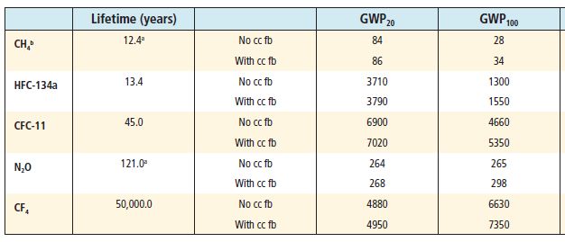
Table of Contents

1. Introduction ................................................................................................................................... 4
2. Material and methods ................................................................................................................... 5
3. Theory/calculation ........................................................................................................................ 6
 3.1. Global warming potentials of GHGs ...................................................................................... 6
 3.2. Aerosol cooling .................................................................................................................... 12
 3.3. Heating potentials of fossil fuels considering GWPins of methane .................................... 14
 3.4. Opportunity costs for unused carbon sinks ........................................................................ 15
 3.5. Deforestation....................................................................................................................... 17
 3.6. Capture fisheries and aquaculture ...................................................................................... 18
 3.7. Pre-production, processing and post-production ............................................................... 19
4. Results ......................................................................................................................................... 20
 4.1. Today's methane emissions have more immediate significance than today’s CO2 emissions
 20
 4.2. Animal agriculture is the biggest cause of global warming ................................................. 20
5. Conclusions.................................................................................................................................. 23
6. Discussion .................................................................................................................................... 24
7. Appendix...................................................................................................................................... 25
 A) Comparison of different studies/reports on the role of animal agriculture / livestock farming
 in climate change ............................................................................................................................ 25
 B) Calculation of contributions of animal agriculture (AA) and fossil fuel based industries to
 climate change as assumed by FAO and IPCC (supporting Fig. 4) ................................................... 26
8. Acknowledgments ....................................................................................................................... 27
9. References ................................................................................................................................... 28
10. Funding .................................................................................................................................... 30

M. Müller Page 2 of 30 02 January 2021

Table of Tables

Table 1: RF of anthropogenic WMGHG in 2020 .................................................................................... 7
Table 2: Interim results of annual contributions of major GHGs to RF in 2020 (4 s.f.) ....................... 10
Table 3: Calculation of GWPins for CH4 and N2O using Radiative Efficiency (RE) averaged over the last
10 years ............................................................................................................................................... 11
Table 4: Calculation of the 2011 annual contributions of major aerosols to ERF based on GWP10 (4
s.f.) ....................................................................................................................................................... 13
Table 5: Calculation of relative climate heating potentials of the major fossil fuel sources (3 s.f.) ... 15
Table 6: Calculation of annual opportunity costs in terms of CO2 emissions per year for unused
carbon sinks of the current agriculture system vs.a fully plant-based system (4 s.f.) ........................ 16
Table 7: Calculation of annual CO2 emissions from deforestation for animal agriculture (3 s.f.) ....... 17
Table 8: Determination of most harmful industries to climate heating (3 s.f.) .................................. 22

Table of Figures

Fig. 1: RF in 2011 as depicted in IPCC’s Fifth Assessment Report (AR5) and values of anthropogenic
forcing.................................................................................................................................................... 6
Fig. 2: GWPs calculated by IPCC AR5 for H=20 and H=100 .................................................................. 8
Fig. 3: Relative significance of GHGs, for the current composition of the atmosphere and the RFs
(a.), for a one-time pulse and stretching over 100 years (b.) and for the current emissions and
immediate heating effects (c.) ............................................................................................................ 20
Fig. 4: Previously assumed major causes of global warming vs. actual major causes after revaluation
............................................................................................................................................................. 23
Fig. 5: Comparison of different studies on the role of animal agriculture / livestock farming in global
warming............................................................................................................................................... 25
Fig. 6: Calculation of contributions of animal agriculture and fossil-fuel-based industries to climate
change as assumed by FAO and IPCC (supporting Fig. 4).................................................................... 26

M. Müller Page 3 of 30 02 January 2021

1. Introduction

The problem of climate heating is attracting more and more attention within politics and wider
society. The fossil fuel industry is generally seen as the main cause and focus for action. Scientists
too present burning fossil fuels, be it for energy production, heating or transportation, as central to
the greenhouse effect, and thus reducing fossil fuel consumption is promoted as almost the only
solution.

This assumption is based on authoritative reports from official bodies like the Intergovernmental
Panel on Climate Change (IPCC). Most derivative studies and literature refer to reports by the IPCC
and do not question the major statements thereof.

By investigating the greenhouse gas (GHG) emissions of fossil-fuel-combusting industries on the
one hand, and animal agriculture1 on the other, it is shown here that conclusions of the causes for
climate heating made by scientists are often based on technically correct but irrelevant
calculations, omission of physical effects, negligence of opportunity costs and imprecisely allocated
inputs.

1Animal agriculture sometimes is understood to consist of livestock farming, aquaculture and capture fisheries. Here, the
term “animal agriculture”, includes livestock farming and aquaculture, while capture fisheries is excluded (for details see
chapter 3.6).

M. Müller Page 4 of 30 02 January 2021

2. Material and methods

The research for this paper focused on the analysis of the major reports and studies on the
contributions of animal agriculture and fossil-fuel-based industries to global warming as well as
reviews of used input data, models and calculation models.

As for animal agriculture, reports, studies and input data were mainly from the Food and
Agriculture Organisation (FAO), the Worldwatch Institute (WWI), the Intergovernmental Panel on
Climate Change (IPCC) and the Global Change Data Lab (Our World in Data). Regarding the fossil-
fuel-based industries major reports, studies and input data analyzed were from the IPCC, the
International Energy Agency (IEA) and the Global Change Data Lab.

Most of the data used for the calculations are primary data, i.e. measured data. Some more
complex input data are from studies that are referred to.

All used input data and calculation methods are directly referenced in detail at the appropriate
positions in the text. All calculations can be reproduced in the Excel sheets which are part of the
supplementary file to this paper.

The resulting mathematical model is also migrated to a website which allows the input of latest
data and simulation of different scenarios: https://www.industryfootprint.org/, PW: vh54$3gd321

M. Müller Page 5 of 30 02 January 2021

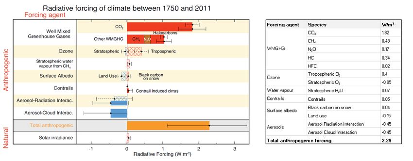
3. Theory/calculation

3.1. Global warming potentials of GHGs

The human-induced greenhouse effect is caused by hundreds of different GHGs and a few aerosols.
It is directly measured with sensors in the atmosphere, but also simulated in laboratories and
mathematical models [1]. The effect can be expressed as anthropogenic Radiative Forcing (RF),
which is the additional energy per second trapped in the atmosphere by GHGs and aerosols emitted
due to human activities. According to NOAA/ESRL's Global Monitoring Division, the uncertainties of
the models are of about 10%2. Fig. 1 shows the RF in 2011 due to changes in the atmosphere
compared to pre-industrial levels in 1750 [2].

 Fig. 1: RF in 2011 as depicted in IPCC’s Fifth Assessment Report (AR5) and values of anthropogenic forcing

It is essential to take into account that the RF indeed does reflect the effect of the human-caused
composition of forcing agents in the atmosphere, which is the result of all human-caused emissions
and their absorption and decay since 1750. Yet, the RF does not reflect the greenhouse effect due
to current GHG emissions and aerosols.

The 2020 RF values for anthropogenic ‘Well-Mixed Greenhouse Gases (WMGHGs)’ are presented in
Table 1, being determined as follows:

(1) The 2020 mole fractions of CO2 are retrieved from NOAA/ESRL3. The RF4 is calculated using the
expressions based on radiative transfer models [3].

2 Global Monitoring Laboratory (GML) of the National Oceanic and Atmospheric Administration (USA)
3 Data is taken from https://www.esrl.noaa.gov/gmd/ccgg/trends; another data hub is https://gaw.kishou.go.jp
4 RF= α×ln(C C -1), where α=5.35, C =278ppm and C is global mean atmospheric concentration of CO in 2020
 0 0 2

M. Müller Page 6 of 30 02 January 2021

(2) The 2020 mole fractions of CH4 retrieved from NOAA/ESRL. The direct RF5 is calculated using the
expressions based on radiative transfer models [3]. The current concentration of methane alone
has RF of 0.519 W m-2. However, since methane has indirect effects on other GHGs, the actual RF of
methane is almost twice as high, which is 1.013 W m-2:

 - CH4 has indirect effects to tropospheric and stratospheric ozone which is estimated to be
 additional 50% to the direct effect [4].
 - CH4 changes stratospheric H2O being about 15% of the direct effect [4].
 - CH4 interacts with sulphate and degrades this cooling aerosol, which accounts for a further
 30% forcing above the direct effect [5].
 - CH4 finally decomposes to CO2. Since the amounts are small, the forcing effects (< 1%) are
 not specifically integrated in the models.
 - Experiments showed that increases in global methane emissions cause significant decrease
 in hydroxyl, leading to a negative feedback loop for CH4 decomposition and thus increasing
 CH4 potency [5]. Due to uncertainties regarding the magnitude of the effect they are not
 include here.

(3) The 2020 mole fractions of N2O are retrieved from NOAA/ESRL. The direct RF6 is calculated using
the expressions based on radiative transfer models [3].

(4) The 2018 RF values of other WMGHGs (CFC12, CFC11, 15-minor)7 are retrieved from
NOAA/ESRL8 and is extrapolate to 2020, based on the 10yr average rate of change (+0.41% yr-1).

 Forcing
 No. WMGHG
 Factor (W m-2)
 (1) CO2 2.116
 (2) CH4 1.013
 abundant 0.519
 increase in tropospheric and stratospheric ozone 0.50 0.260
 increase in stratospheric H2O 0.15 0.078
 decrease in sulfate 0.30 0.156
 (3) N2O 0.206
 (4) HC/HFC 0.349
 Table 1: RF of anthropogenic WMGHG in 2020

Considering the atmospheric composition of anthropogenic WMGHGs in 2020, CO2 contributes to
global heating by 57%, CH4 by 28%, N2O by 6% and Halocarbons (HC) and Hydrofluorocarbons (HCF)
by 9%.

5 RF=β×(M½ - Mo½) - [f(M,No) - f(Mo,No)], where β=0.036, Mo=722ppb, N0=270ppb, and M is global mean atmospheric
concentration of CH4 in 2020, f(M,N) = 0.47×ln[1 + 2.01x10-5 (M×N)0.75 + 5.31x10-15M×(M×N)1.52]
6 RF=ε×(N½ - N ½) - [f(M ,N) - f(M ,N )], where ε=0.12, M =722ppb, N =270ppb, and N is global mean atmospheric
 o o o o o 0
concentration of N2O in 2020, f(M,N) = 0.47×ln[1 + 2.01x10-5 (M×N)0.75 + 5.31x10-15M×(M×N)1.52]
7 Other WMGHGs are mainly chlorofluorocarbons e.g. used as refrigerants, solvents in dry cleaning, propellants in spray

cans and blowing agents for expanded plastic products. Production and use has significantly decreased over decades,
however, due to their very long lifetime they still play a significant role as forcing agents. Halons were developed for the
extinguishing of electrical fires.
8 www.esrl.noaa.gov/gmd/aggi/aggi.html

M. Müller Page 7 of 30 02 January 2021

This consideration does not provide answers to the contribution of current emissions to global
heating since all gases have different lifetimes in the atmosphere and were emitted to different
extents in the past. To overcome this issue the IPCC introduced the concept of Global Warming
Potentials (GWP) for different GHGs in relation to CO2 [6]. The GWPs are calculated as follows:
 
 ∫0 ( ) 
 ( ) = .
 ∫0 2 ( ) 

With this method the effect of a one-time pulse of GHG i, leading to RFi is integrated over H years
and related to the integration of the effect of a one-time pulse of CO2 leading to RFCO2 [39].

With GWPs it can be calculated how much more energy a one-time pulse of a certain mass of gas
traps in the atmosphere relative to the same mass of CO2 over a defined period.

Since decays of different isolated GHGs are well known it is straightforward to calculate GWPs for
different periods. The IPCC provided some GWPs for random periods as shown in Fig. 2 [7].

 Fig. 2: GWPs calculated by IPCC AR5 for H=20 and H=100 9

In all IPCC reports and diagrams for all GHGs and aerosols, the period of 100 years was chosen to
calculate the GWP. Most citations and follow-up papers and studies, as well as nearly all press
releases and articles, are based on GWPs calculated for a period of 100 years. Even national and
supra-national decisions and declarations of intent (e.g. the Paris climate agreement) primarily use
GWPs calculated for 100 year periods.

However, there is no single argument to choose a period of 100 years or any other period. The IPCC
itself states in its Fifth Assessment Report (AR5) [8]:

 “The GWP has become the default metric for transferring emissions of different gases to a common scale;
 often called ‘CO2 equivalent emissions’ (e.g., Shine, 2009). It has usually been integrated over 20, 100 or
 500 years consistent with Houghton et al. (1990). Note, however that Houghton et al. presented these
 time horizons as ‘candidates for discussion [that] should not be considered as having any special
 significance’. The GWP for a time horizon of 100 years was later adopted as a metric to implement the
 multi-gas approach embedded in the United Nations Framework Convention on Climate Change (UNFCCC)
 and made operational in the 1997 Kyoto Protocol. The choice of time horizon has a strong effect on the
 GWP values — and thus also on the calculated contributions of CO2 equivalent emissions by component,
 sector or nation. There is no scientific argument for selecting 100 years compared with other choices
 (Fuglestvedt et al., 2003; Shine, 2009).”

9
 Most studies and reports use GWP100 without climate carbon feedbacks (cc fb). Climate carbon feedbacks (warming-
induced release of CO2 from the land biosphere and ocean) inflate the GWPs of non-CO2 GHGs by about 20% for long-
term considerations. Since the focus in this analysis is on instantaneous RF, climate carbon feedbacks are not included in
the calculations.

M. Müller Page 8 of 30 02 January 2021

Calculating the total effect of a one-time pulse of GHGs over a certain time horizon may give
interesting answers to hypothetical situations, e.g. TCOs10 for economic views. However, GHGs are
emitted constantly, balancing out depletions and decays, or leading to decreasing or increasing
concentrations in the atmosphere and resulting in the RF that are observed today.

Therefore, the question to answer is: how much do currently emitted GHGs contribute to current
climate heating?

To answer this question, it is best to use directly observed data and apply straightforward
calculations, as follows:

(1) The RFs of the human-caused concentrations of GHGs in the atmosphere are known from the
calculations above. The focus here and in the following investigations is on the three main gases
emitted by animal agriculture and the fossil fuel industries. Other gases such as HCs and HFCs are
emitted by manufacturing processes and product use, but emissions have been significantly and
steadily reduced in recent decades.

(2) The abundance-based relative importance of each of the three major GHGs is calculated.

(3) The human-caused rise of major GHG levels in the atmosphere are retrieved from NOAA/ESRL,
implicitly factoring in depletions and decays.11

(4) The human-caused amount of GHGs being in the atmosphere at present is calculated.12

(5) The RFs for unit masses of GHGs are calculated.

(6) The instantaneous GWPins, being effective in the present and not being stretched over a period
is calculated.13

(7) The annually emitted amounts of GHGs are retrieved from the 2019 IPCC report [9].

(8) The annual contribution of each GHG to the overall RF is calculated.14

(9) The emission-based relative importance of each of the three major GHGs is calculated.

10
 Total Cost of Ownership: financial estimate to determine the direct and indirect costs of a product or system
11 Data is retrieved from https://www.esrl.noaa.gov/gmd/ccgg/trends; another data hub is https://gaw.kishou.go.jp
12 The total mean mass of the atmosphere m 18
 atmos without water vapour is 5.1352 x 10 kg [34]. Abundance increases
(ABI) are given in table 2, No. 3. Molar masses M of all gasses are calculated from standard atomic masses. The average
molar mass of air (Mair) in the atmosphere is 28.9656 g molair-1 (4 d.p.) [35]. The total mass increases of CH4, CO2 and N2O
in the atmosphere are calculated as follows: 1750−2020 = × × × −1 .
13 GWP -1 1 -1 1 -1 -1
 CH4 = (RFCH4 Gt ) x (RFCO2 Gt- ) , GWPN2O = (RFN2O Gt- ) x (RFCO2 Gt )
14 (Emissions (Gt) Yr-1) × (RF (W m-2) Gt-1)

M. Müller Page 9 of 30 02 January 2021

GHG
 No. CH4 CO2 N2O
 Value/Calculation

 (1) RF (W m-2) 1.013 2.116 0.2061
 (2) Share 30% 64% 6%
 (3) Rise (ppm) 1.155 134.9 0.0632
 (4) Amount (Gt) 3.285 1053 0.493
 (5) RF ((W m-2) Gt-1) 0.3083 0.002011 0.4180
 (6) GWPins 153.3 1 207.9
 (7) Emissions (Gt Yr-1) 0.362 39.1 0.0106
 (8) Annual Contr. to ERF (W m-2) 0.1116 0.07862 0.004431
 (9) Share 57.3% 40.4% 2.3%
 Table 2: Interim results of annual contributions of major GHGs to RF in 2020 (4 s.f.)

Interim results (1):

 Ref. (No. 2) and (No. 9): Considering the yearly emitted amount of methane rather than its
 current abundance in the atmosphere almost doubles its significance as a GHG. This is a result of
 its short lifetime of about 12.4 years. The significance of CO2 drops by a third and that of N2O by
 two thirds which can be explained by the long lifetimes of > 200 and 121 years respectively. The
 contributions of very long-lived GHGs like HCs and HCFs to current emission-based RF are very
 low due to low and declining emissions. Their contributions to current abundance-based RF are
 mostly caused by past emissions.
 Ref. (No. 6): The GWP of methane used by IPCC, throughout scientific world and media is 28 on
 a 100 year time horizon. Without integration over time, however, the instantaneous GWPins of
 methane is 153. It emerges that it is higher than the initial GWP0 of ~120 according to models
 used by the IPCC. This is due to the findings of Shindell et al., that a rise in global methane
 emissions showed decreases in sulphate particles, playing a crucial role in the depletion of
 methane [5].

With the above calculations certain GWPins of CH4 and N2O relative to CO2 are obtained. With the
method used, however, current Radiative Efficiencies (RE)15 due to current band saturations16 in the
atmosphere were not taken into account. Instead, REs averaged over concentration changes
between the years 1750 and 2020 were put into relation.

To determine the GWPins for current GHG saturation levels recent RF changes must be put in
relation to recent abundance changes.17

(1) The atmospheric concentrations (AC) of all GHGs are retrieved from NOAA/ESRL.

(2) All RFs are calculated (see footnotes 4,5,6).

(3) The respective molar masses M are known.

15 RE is the radiative forcing per unit mass increase in atmospheric abundance of a defined forcing agent [10].
16 REs decrease with increased band saturations of defined forcing agent. This is reflected in the models to calculate RFs
(see footnotes 4,5,6).
17 In order to balance out inaccuracies in annual concentrations a period of 10 years was chosen to average the values.

M. Müller Page 10 of 30 02 January 2021

(4) The Radiative Efficiencies averaged over the period 1750 – 2020 are calculated,

 RE[GHG]270 = (( 2020 − 1750 ) × ( 2020 − 1750 )−1 ) × −1 ,

 and following the GWPins of CH4 as its RE in relation to that of CO2. The GWPins of N2O is to be
 calculated differently in order to consider CH4 reductions in the atmosphere due to increased
 N2O abundance [4]. The REN2O is to be corrected by the following expression:

 1 − 0.36 × 1.95 × (( 2020 − 1750 ) × ( 2020 − 1750 )−1 ) 4 × (( 2020 − 1750 ) ×
 −1
 ( 2020 − 1750 )−1 ) .
 2 

(5) The Radiative Efficiencies averaged over the period 2010 – 2020 are calculated,

 RE[GHG]10 = (( 2020 − 2010 ) × ( 2020 − 2010 )−1 ) × −1

 and following the GWPins of CH4 as its RE in relation to that of CO2. The GWPins of N2O is to be
 calculated differently in order to consider CH4 reductions in the atmosphere due to increased
 N2O abundance [4]. The REN2O is to be corrected by the following expression:

 1 − 0.36 × 1.95 × (( 2020 − 2010 ) × ( 2020 − 2010 )−1 ) 4 × (( 2020 − 2010 ) ×
 −1
 ( 2020 − 2010 )−1 ) .
 2 

(6) The changes in the Radiative Efficiencies between the averages of the period 2010 – 2020 to the
 averages of the period 1750 – 2020 are calculated.

 GHG CH4 CO2 N2O
 No.
 Value/Calculation Value Unit Value Unit Value Unit

 Abundance (AB) in 1750 0.722 ppm 278.0 ppm 0.2700 ppm
 (1) Abundance (AB) in 2010 1.799 ppm 388.6 ppm 0.3231 ppm
 Abundance in 2020 1.877 ppm 412.9 ppm 0.3332 ppm
 RF in 1750 0 W m-2 0 W m-2 0 W m-2
 (2) RF in 2010 0.9569 W m-2 1.792 W m-2 0.1746 W m-2
 RF in 2020 1.013 W m-2 2.116 W m-2 0.2061 W m-2
 (3) Molar mass 16.04 g mol-1 44.009 g mol-1 44.01 g mol-1
 ((W m-2) ppm-1) ((W m-2) ppm-1) ((W m-2) ppm-1)
 RE 1750-2020 0.05465 0.0003565 0.07411
 (4) (g mol-1)-1 (g mol-1)-1 (g mol-1)-1

 GWPins (1750-2020) 153.3 1 168.7

 ((W m-2) ppm-1) (W m-2) ppm-1)/ ((W m-2) ppm-1)
 RE 2010-2020 0.04444 0.0003034 0.07091
 (5) (g mol-1)-1 (g mol-1) (g mol-1)-1

 GWPins (2010-2020) 146.4 1 196.2
 (6) RE change -19% -15% -4%
 Table 3: Calculation of GWPins for CH4 and N2O using Radiative Efficiency (RE) averaged over the last 10 years

Interim results (2):

 Compared to the first calculation method, the GWPins of CH4 and N2O change slightly:
 - the GWPins of CH4 drops to about 146 from 153
 - the GWPins of N2O drops to about 196 from 208.

M. Müller Page 11 of 30 02 January 2021

 The reasons for the changes in the GWPs are the different REs in the different periods and the
 integration of indirect effects for N2O:
 - The RE of CH4 (period 2010 – 2020 vs. period 1750 – 2020) drops more than that of CO2
 (19% vs. 15%). This is because of a higher saturation effect of CH4 compared to that of CO2.
 - The RE of N2O (period 2010 – 2020 vs. period 1750 – 2020) drops less than that of CO2 (4%
 vs. 15%). This is because of a lower saturation effect of N2O compared to that of CO2.
 - Increased N2O abundance lead to a reduction of CH4 in the atmosphere (-36 molecules per
 +100 molecules N2O) [4].

The GWPins (146.4) for the period 2010 – 2020 are used in all following calculations.

3.2. Aerosol cooling

In addition to heat-trapping gases, other anthropogenic emissions can impact the climate by
scattering and absorbing shortwave and longwave radiation and/or by enforcing cloud albedo.
These aerosols almost entirely originate from fuel combustion and biomass burning and thus are
strongly related to fossil- and biofuel-caused CO2 emissions.

Radiative forcing of aerosols can be caused by

  aerosol–radiation interaction (ARI), also denoted as direct aerosol effect
  aerosol–cloud interaction (ACI), also denoted as cloud albedo effect

As indicated in Fig. 1, in 2011 atmospheric composition of aerosols both ARI and ACI had cooling
effects of 0.45 W m-2 each. Analog to GHGs above, these figures represent the effect of all human-
caused emissions since 1750, but not the effect due to emissions.

Unlike the major GHGs, there are no data of averaged global atmospheric concentrations of
aerosols18, so that it is not possible to calculate instantaneous GWPs as done above. The best
available data are 2011 model-based GWPs of the five major aerosols for one-time pulses and
radiative forcing periods of 10 years [11], the following calculations can be done:

(1) There are estimates of the yearly emissions of major aerosols [12].

(2.1) There are estimates of GWPs over 10 years [11]. These only relate to ARI, not to ACI.

(2.2) The RF Gt-1 for each aerosol (ARI), using the RF Gt-1 of CO2 (0.002012 W m-2) as determined in
table 2 is calculated.

(2.3) The annual contribution of each aerosol to ERF is calculated and summed up to get the total
ARI. The ACI can be calculated using factor 1.125 [13].

(3.1, 3.2, 3.3) The same can be calculated for GWPs over 100 years.

18Aerosols are only strongly emitted at hotspots and are very short-lived, so that they do not mix uniformly in the
atmosphere. It is therefore difficult to measure them and determine mean values.

M. Müller Page 12 of 30 02 January 2021

Aerosol
 Black Organic
 SO2 Total Total
 No. Carbon Carbon NOX CO
 (H2SO4) (ARI) (ARI&ACI)
 (BC) (OC)
 Value/Calculation
 (1) Emissions (Gt Yr-1) 0.005310 0.01360 0.1270 0.03720 0.8930
 (2.1) GWP10 4349 -438.5 -253.5 134.2 8.600
 (2.2) RF10 ((W m-2) Gt-1) 8.751 -0.8823 -0.5101 0.2700 0.01730
 (2.3) RF10 (W m-2) 0.04647 -0.01200 -0.06478 0.01004 0.01545 -0.004813 -0.01023
 (3.1) GWP100 658.6 -66.4 -38.4 -10.8 1.9
 (3.2) RF100 ((W m-2) Gt-1) 1.325 -0.1336 -0.07726 -0.02173 0.003823
 (3.3) RF100 (W m-2) 0.007037 -0.001817 -0.00981 -0.0008084 0.003414 -0.001987 -0.004223
 (4) Lifetimes (years) 0.01923 0.0001142 1.5 0.0004338 0.3333
 Table 4: Calculation of the 2011 annual contributions of major aerosols to ERF based on GWP10 (4 s.f.)

Interim results:

 Unlike the significant cooling effect of 0.9 W m-2 (ARI & ACI combined), representing a 31%
 cooling to the RF of the three main atmospheric GHGs CH4, CO2 and N2O in 201119, the effect
 with perspective to emitted GHGs seems to be much smaller. If ARI & ACI with GWP10 are put
 into relation with the RF contributions of emitted GHGs in 2011, they only lead to a cooling of
 about 5%20. There are at least two explanations:
  First, this relation cannot really be made since the RF of emitted GHGs and the RF of
 aerosols integrated over 10 years are not comparable. Data for the RF of currently emitted
 aerosols are not (yet) available (due to a lack of data for atmospheric concentrations), but
 as aerosols follow exponential decay, it is possible that their RF would have higher cooling
 effects.
  Second, this big discrepancy between the cooling of aerosols existent in the atmosphere
 and aerosols emitted emerges from the short lifetime of the strongest heating aerosol,
 Black Carbon (BC), in contrast to the much longer lifetime of the strongest cooling aerosol,
 SO2, which decomposes to sulphate (H2SO4). It seems that the strong cooling net effects of
 aerosols are legacies of huge past emissions of SO2.
 While there is confidence in the overall net cooling effect of aerosols of 0.9 W m-2 due to
 atmospheric composition [14], there are high uncertainties regarding emission based aerosol
 effects. This is because there is no data of globally averaged aerosol concentrations and because
 of a lack of understanding of highly complex decomposing and feedback processes.
 Even though it is likely that there is significant cooling due to currently emitted aerosols, these
 effects are not included in the overall calculations due to the high uncertainties on their
 magnitudes. If this were done, however, the impact of fossil-fuel-based industries on climate
 heating would be further weakened because of their role as the major cause for all aerosols.

19 By using factor 1.95 as calculated in 3.1, indirect effects of CH4 lead to a 2011 RF of 0.936 W m-2. Therefore the
calculation is (-0.9 W m-2) / (2.926 W m-2).
20 The calculation is: (-0.01023 W m-2) / (0.1116 W m-2 + 0.07867 W m-2 + 0.004434 W m-2).

M. Müller Page 13 of 30 02 January 2021

3.3. Heating potentials of fossil fuels considering GWPins of methane

Significant amounts of CH4 are emitted from all major fossil fuel energy sources. CH4 is released
through exploitation, processing, transport and combustion of coal, oil and gas. While reasons
(fugitive and vented emissions and emissions resulting from incomplete combustion, i.e. flaring)
vary heavily among energy sources and the amount of energy production per energy source is
different, overall methane emitted by coal, oil and gas is almost shared equally.

Using data on energy extracted by coal, oil and gas mining, data on emissions and the GWPins of
methane, the rise in heating potentials of fossil fuels compared to the prevalent assumptions can
be determined:

(1) The global energy production21 in terms of TPES22 (overall production excluding stock changes
and bunkers) can be retrieved International Energy Agency using the energy balance from 2017
[32].23

(2) The GWP100 as used by IPCC is 28, the GWPins as calculated in chapter 3.1 is about 146.

(3) The methane emissions of coal, oil and gas is estimated to be about 40 Mt each [32].

(4) The CO2eq of the methane emissions is calculated.

(5) The CO2 emissions by energy source can be retrieved from International Energy Agency [32].

(6) The total CO2eq emissions is calculated per energy source.

(7) The climate effective emissions per energy unit is calculated

- for considerations with a GWP of methane being stretched over 100 years
- for considerations with an instantaneous GWP of methane.

(8) Based on the results of No. (7), it can be determined how the consideration of methane with
GWPins increases the emissions of CO2eq per energy unit in contrast to when GWP100 is applied.

(9) Based on the results of No. (7), the output of coal and gas emissions per unit of energy can be
put in relation to that of oil emissions (aerosol cooling effects are not considered here).

21 Energy production is the used term in the energy balances of the fossil fuel mining industry and refers to the energy
contained in oil, coal and gas extracted from the ground.
22 TPES: Total Primary Energy Supply
23 It is to be noted that this is the energy supply of each source and not the energy consumption. Energy consumption is

much lower due to energy losses along the exploitation chain and different energy efficiencies (e.g. power plants,
combustion engines).

M. Müller Page 14 of 30 02 January 2021

Energy Source
 No. Coal Oil Gas
 Category
 (1) Energy production (PWh) 44.1 51.7 36.1
 (2) GWP GWP100 GWPins GWP100 GWPins GWP100 GWPins
 (3) Emissions ((Gt CH4) yr-1) 0.04 0.04 0.04 0.04 0.04 0.04
 (4) Emissions ((Gt CO2eq) yr-1) 1.12 5.86 1.11 5.80 1.11 5.80
 (5) Emissions ((Gt CO2) yr-1) 14.5 14.5 11.4 11.4 6.74 6.74
 (6) TOTAL (CH4 + CO2) 15.6 20.4 12.5 17.2 7.85 12.5
 (7) Gt CO2eq (PWh (kg kWh-1))-1 0.354 0.462 0.241 0.332 0.217 0.347
 (8) Rise in heating potential 30% 38% 60%
 (9) GHG efficiency relative to oil 1.47 1.39 1 1 0.90 1.05
 Table 5: Calculation of relative climate heating potentials of the major fossil fuel sources (3 s.f.)

Interim results:

 CO2eq emissions per energy unit is by far worst for coal in all scenarios. Using GWPins in the
 calculations reveals that the ratio is best for oil with 332 g Wh-1. This is different to previous
 assumptions, where gas is seen to be most GHG efficient.
 Using GWPins for methane increases the heating potentials for coal by 30%, for oil by 38% and
 for gas by 60%. The different increases occur because the total amount of CO2 emissions are
 highest for coal, followed by oil, and are lowest for gas.
 Previous assumptions are, that the combustion of gas is about 20% more GHG efficient than oil
 and about 40% compared to coal [32]. Applying GWPins shows, that gas is about 5% less GHG
 efficient than oil.

3.4. Opportunity costs for unused carbon sinks

Almost all studies, including all IPCC reports consider land use by animal agriculture as a given and
constant fact. If at all, land use is only taken into account regarding changes compared to former
years. It is scientific consensus that food production through animals requires multiples of
resources compared to plant-based alternatives and thus is highly inefficient. Around 83% of
agricultural land is used for meat, aquaculture, eggs and dairy (animal feed and grazing) but it
provides only 18% of food calories and 37% of protein for human consumption [15]. Plant-based
nutrition is both healthiest and least contributory to climate heating [16]. Animal products are not
necessary for human nutrition and health. On the contrary, they are causes for certain health
conditions, including ischemic heart disease, type 2 diabetes, hypertension, certain types of cancer
and obesity [17]. Therefore, land used for animal agriculture could be freed extensively. Without
needless animal agriculture global farmland use could be reduced by more than 76% [15].

Land used for animal agriculture then represents opportunity costs, i.e. costs for unused
alternatives, e.g. for carbon sinks.

The opportunity costs (in terms of CO2 emissions per year) for unused carbon sinks of the current
agriculture system vs. a plant-based system can be determined as follows:

M. Müller Page 15 of 30 02 January 2021

(1) The global agricultural land can be retrieved from FAO [18].

(2) The area of land used for animal agriculture is about 83% of the overall agricultural land [15].

(3) The area of land freed up by eliminating animal agriculture and switching to a fully plant-based
food system is 76% of the land used for animal agriculture [15].

(4) The area of land that can be reforested24 and the total sequestration potential per year can be
calculated [19],[20].25

(5) The difference between No. 3 and No. 4 is the area of land that can turn back into grassland.
The sequestration potential of grassland per square meter per year [21],[22]26 and the overall
sequestration potential of grasslands can be calculated.

Finally the total sequestration potential per year is calculated.

 Sequestration Sequestration
 Area
 No. (Potential) land use Potential / m2 Potential

 M km2 (CO2 (kg m-2)) yr-1 (CO2 (Gt)) yr-1
 (1) Agricultural land 51.00
 (2) Land use for animal agriculture 42.33
 (3) Land freed up with plant-based food system 32.17
 (4) thereof qualified for forests 2.848 1.493 4.252
 (5) thereof qualified for grasslands 29.32 0.2455 7.199
 Total sequestration potential 11.45
 Table 6: Calculation of annual opportunity costs in terms of CO2 emissions per year for unused
 carbon sinks of the current agriculture system vs.a fully plant-based system (4 s.f.)

Interim results:

  Animal products for human consumption are not necessary. On the contrary, their production
 and intake have huge disadvantages for the environment, human health and animal wellbeing.
 Even though the environmental damage goes far beyond GHGs, only the opportunity costs in
 terms of missed CO2 sinks are explored here.
 Switching to a plant-based food system releases an area of more than 32 million square
 kilometres. A smaller part can be reforested and a bigger part can transform back to grassland.
 The result of about 11.45 Gt CO2 calculated here as sequestration potential is close to the result
 obtained by a different calculation method used by Goodland and Anhang of the Worldwatch
 Institute in 2009 [23]. In their study they summed up CO2 exhaled by grazing livestock (8.8 Gt
 CO2) and the CO2 sinks missed due to land use for grazing and feeding (2.7 Gt CO2). The
 argumentation of the FAO that respiration by livestock is offset by photosynthesis is true,

24 According to Bronsen et al., a total of 6.78 M km2 of land could be reforested of which to date 42% is grazing land.
25 According to Bronsen et al., a total of 10.124 (Gt CO2) yr-1 could be sequestrated by reforested land, of which to date
42% is grazing land.
26 According to Michael Abberton et al., and Janssens, I. A. et al., the mean grassland sequestration for carbon is

67 ( −2 ) −1 , so that the CO2 sequestration potential is: 0.067 (kg −2 ) −1 × 44.01 g −1 × (12.01 g −1 )−1 .

M. Müller Page 16 of 30 02 January 2021

however respiration accounts for net opportunity costs, since without livestock CO2 sequestered
 by photosynthesis is permanently stored in the soil.
 According to Hayek et al. (2020) the carbon opportunity costs of animal-sourced food
 production on land over 30 years are 332–547 Gt CO2 which is equivalent to 11.1-18.2 Gt CO2 per
 year [40].

3.5. Deforestation

Animal agriculture requires the vast majority of agricultural land. In order to balance crop failures
caused by climate change, soil degradation and biodiversity loss, and to increase the production of
animal products, further land is needed every year and made available by deforestation.

Deforestation for animal agriculture is often mentioned in IPCC reports or in studies by the Food
and Agriculture Organization (FAO), but is usually not fully taken into account or imprecisely
assigned (see appendix).

The CO2 emitted per year by burning forests for animal agriculture is calculated as follows:

(1) The total CO2 emission reduction potential resulting from ending deforestation can be retrieved
from the IPPC Special Report on climate change [24].

(2) The portion for commercial crop production for animal agriculture is calculated [25], [26].27

(3) The portion for commercial cattle ranching can be retrieved from The UNFCC [26].

(4) The portion for small scale animal agriculture is calculated [15], [26].28

Finally the total annual CO2 emission reduction potential achievable by stopping deforestation for
animal agriculture is calculated.

 No. Deforestation Portion (CO2 (Gt)) yr-1

 (1) Overall reduction potential from ending deforestation 5.20
 (2) therof with commercial crops for livestock 6.60% 0.343
 (3) therof with commercial cattle ranching 12.0% 0.624
 (4) therof with small scale animal agriculture 34.9% 1.81
 Reduction potential from ending deforestation for animal agriculture 53.5% 2.78
 Table 7: Calculation of annual CO2 emissions from deforestation for animal agriculture (3 s.f.)

27 According to UNFCCC United Nations Framework Convention on Climate Change, 2007, about 20% of all deforestation
is due to commercial crop production. According to United Nations Food and Agricultural Organization, 2006, about 33%
of overall crop production is for livestock feed. Therefore, it was projected that commercial crop production for animal
agriculture accounts for at least 6.6% of deforestation.
28 According to UNFCCC United Nations Framework Convention on Climate Change, 2007, about 42% of all deforestation

is due to small scale agriculture. According to Poore et al., 2018, about 83% of overall agricultural land is for animal
agriculture. Therefore, it was projected that small scale agriculture (animal feed and grazing land) accounts for about
34.9% of deforestation.

M. Müller Page 17 of 30 02 January 2021

Interim results:

 According to the World Bank, at the average global forests have decreased by 0.051 M km2 per
 year over the last 30 years [27]. The major cause for deforestation has been and is animal
 agriculture. More than half of global deforestation is for additional grazing land and land to grow
 additional animal feed.29
 Annually about 2.8 Gt of CO2 is released to the atmosphere due to deforestation for animal
 agriculture. This number is a little bit higher than the 2.4 Gt CO2 as calculated by the 2006 study
 from FAO [28]. A reason might be that FAO excluded Argentina because of lack of data.

3.6. Capture fisheries and aquaculture

In some studies and reports only livestock is considered for the GHG emissions in animal agriculture
(see appendix). However, 39% of meat production today comes from the fishing industry. In 2015
meat from livestock accounted for 324 M tons and seafood production for 210 M tons. Aquaculture
has been growing exponentially from 2 M tons in 1960 to 106 M tons in 2015, now being even
bigger than capture fisheries (94 M tons) [18].

Similar to land animals, marine animals exhale CO2 and produce excretions becoming GHG
effective. CO2 and GHG effective excretions produced by wild marine animals originate from ocean
plant intake (mostly algae) at the very beginning of the food chain and thus are CO2 neutral. As for
aquaculture, however, a certain portion produced by animals comes from cultivated plants (wheat,
soybean, maize, rapeseed oil, palm oil). These CO2 and GHG effective excretions are GHG net
sources and need to be attributed to animal agriculture. An alternate way to determine these GHGs
is to calculate the carbon sinks of the land needed for plant-based aqua feed. This is (at least
partially) considered in the factor of 0.83 used in 3.4; No. 2, representing the portion of land used
for animal agriculture. About 5 percentage points of this factor can be attributed to aquaculture.30

Aquafeed consists of fish meal, fish oil and plants, with the proportion of vegetable aquafeed
estimated at 30-70% [29]. The estimates are rough and of wide range, but seem to be considerably
higher than those included in the calculations.

It is worth mentioning that due to high costs of animal aquafeed and ocean overfishing a shift to
plant-based aquafeed is currently taking place.

As for marine animals it might be that their withdrawal and consumption are not CO2 neutral since
without such withdrawal dead ocean plants and dead marine animals would sink to the bottom of
the sea and such carbon would be permanently removed from the carbon cycle. Since this vague
assumption is not backed by any reliable data and studies, such CO2 is not included in the
calculations of this analysis.

29
 Deforestation for growing crops for aquaculture feed is not included in the calculations due to lack of reliable data. In
the approximate calculations these CO2 emissions are relatively low.
30 According to Poore, J., Nemecek, T., 2018, livestock and aquaculture requires 83% of agricultural land [15], while

according to United Nations Food and Agricultural Organization, 2006, livestock alone requires 78 % of agricultural land
[36].

M. Müller Page 18 of 30 02 January 2021

3.7. Pre-production, processing and post-production

Some studies and reports include GHG emissions from pre-production, processing and post
production of products. This would require a Life-Cycle-Analysis (LCA) of all products of all sectors.
Although some estimates are available for some industries31 due to high uncertainties and in order
to be consistent across all sectors such data is not included in the calculations of this analysis.

31LCA for agricultural products would include energy (e.g., grain drying, heating in greenhouses), transport (e.g.,
international trade), industry (e.g., synthesis of inorganic fertilisers, manufacturing of farm inputs) and post-production
(e.g., agri-food processing). Pre- to post-production for the whole agricultural sector (excluding fishery) is estimated at
2.6-5.2 Gt CO2 [9]. Specific data for animal agriculture is not available. A conservative LCA for aquaculture results in 0.36
Gt CO2 (with footprints of capture fishery: (1t CO2) x (1t fish)-1, aquaculture: (2.5t CO2) x (1 t fish)-1 [30].

M. Müller Page 19 of 30 02 January 2021

4. Results

4.1. Today's methane emissions have more immediate significance than today’s CO2 emissions

While the long lived GHG CO2 has the potential to trap much energy over a long period of time, its
immediate effect is much smaller than that of CH4. To tackle climate heating it is necessary to focus
on the reduction of those GHGs that have the most impact. The instantaneous climate heating
effect of CH4 in combination with its current amount of emission makes CH4 the GHG of most
significance. In other words, cutting CH4 emissions has more impact than cutting CO2 emissions.

The heating effect of GHGs currently in the atmosphere is depicted in Fig. 3 (a.) The relatively high
importance of CO2 is due to its accumulation over centuries and its long lifetime. The importance of
CO2 as GHG increases heavily in calculations of IPCC when current emissions and GWPs stretched
over 100 years are considered (Fig. 3 (b.)). Taking into account that emitted GHGs are effective
instantaneously reverses the picture and shows that CH4 is indeed the most significant GHG. (Fig. 3
(c.)).

 Fig. 3: Relative significance of GHGs, for the current composition of the atmosphere and the RFs (a.), for a one-time pulse
 and stretching over 100 years (b.) and for the current emissions and immediate heating effects (c.)

4.2. Animal agriculture is the biggest cause of global warming

In chapter 3 the instantaneous GWPs of methane and N2O, the aerosol cooling, unused potential
carbon sinks and often imprecisely allocated major sources of CO2 were investigated. In the
following final calculation only the findings with very strong data basis and high certainty of
accuracy are integrated. Thus, aerosol cooling effects, not precisely known net CO2 emissions of
fisheries, CO2 emissions from pre-production, processing and post production of products and CO2
emissions originated by animal husbandry caused diseases are not included (see appendix).

The final calculation is as follows:

(1) The annually emitted amounts of GHGs are retrieved from the IPCC [9]32. Unused carbon sinks
as calculated in chapter 3.4 are to be added as opportunity costs of animal agriculture. The
ascertained total amount of CO2 is therefore partly not emitted physically but is partly not
sequestered from the atmosphere which has the same effect as emissions. Unsequestered carbon
from avoidable animal agriculture contributes to the greenhouse effect, so it must be considered as
part of the total emissions to which the sectors' emissions are eventually related. For simplicity

32Average for each gas for 2007–2016; estimates are only given until 2016 as this is the latest date when comparable data
are available for all gases

M. Müller Page 20 of 30 02 January 2021

reasons in the following it is not further differentiated between the physical and not sequestered
parts. They are called ‘emissions’ altogether.

(2) The immediate GWPs of all GHGs are taken from the calculations in chapter 3.1.

(3) The CO2eq of each GHG are calculated.

(3.1) Animal agriculture accounts for 33% of global methane emissions [18] and 65% of global N2O
emissions [33]. Unused carbon sinks have been about 11.4 Gt CO2 and animal agriculture caused
deforestation emitted about 2.8 Gt CO2 as calculated in chapters 3.4 and 3.5 respectively.33

(3.2) The focus here is on the major fossil fuel (FF) consuming sectors, which are the energy sector34
and the transportation sector35. In total, fossil fuel combustion annually releases about 119 Mt CH4
(17.4 Gt CO2eq) through coal, oil, gas exploitation, processing and transport. Each energy source
emits about one third of fossil-fuel-caused CH4 (see chapter 3.3).

CH4 emissions in the energy sector are determined by the TPES values ‘Electricity plants’, ‘CHP
plants’ and ‘Heat plants’36 of the 2017 energy balance of the IEA37 [32]. CH4 emissions of the
transportation sector are determined by the TPES values ‘Transport’. CH4 emissions of other sectors
are determined by the remaining TPES values.

The CO2 emissions per sector and the portions of coal, oil and gas in the energy sector are retrieved
from the IEA [32].

The portions of N2O emissions per sector are calculated according to the World Resources Institute
[37]. N2O emissions per energy source are not known (NK).

(3.3) Apart from animal agriculture (AA) and fossil-fuel-based (FF) industries, waste and cultivation
of rice produce make up considerable portions of GHGs. This is due to their high emissions of
methane. Waste accounts for about 9% [31] and rice cultivation for about 4% [18] of the considered
total GHG emissions.

Other sectors comprise housing, industry, forestry, bio-fuels and plant-based agriculture. They
make up the rest and account for about 9% of the totals.

33 Fossil fuel based CO2 emissions for livestock farming have been about 0.3 Gt in 2015 [32]. However, to be consistent
they are not included here since only industry specific emissions across the sectors are considered.
34 Electricity and external heat production (not residential heat)
35 All means of transportation, incl. cars, busses, aircrafts, ships, trucks, etc.
36 CHP: combined heat and power
37 International Energy Agency

M. Müller Page 21 of 30 02 January 2021

GHG CH4 CO2 N2O TOTAL
 No.
 Category abs. % abs. % abs. % abs. %
 (1) Emissions (Gt yr-1) 0.362 50.6 0.0106 n/a n/a
 (2) GWP 146 1 196 n/a n/a
 (3) Emissions ((Gt CO2eq) yr-1) 53.0 100% 50.6 100% 2.08 100% 106 100%
 (3.1) Animal agriculture (AA) 17.4 32.8% 14.2 28.2% 1.35 65.0% 33.0 31%
 Energy (FF) 7.1 13.3% 13.5 26.6% 0.074 3.6% 20.6 19%
 by coal 4.10 8% 9.8 19% < 0.05 NK 13.9 13%
 by oil 0.31 1% 0.72 1% < 0.05 NK 1.03 1%
 (3.2)
 by gas 2.65 5% 2.98 6% < 0.05 NK 5.62 5%
 Transport (FF) 3.78 7.1% 8.04 15.9% 0.0491 2.4% 11.9 11%
 Others (FF) 6.61 12.5% 11.35 22.5% 0.0721 3.5% 18.0 17%
 (3.3) Others (non AA, non FF) 18.2 34.3% 3.48 6.9% 0.532 25.6% 22.2 21%
 Table 8: Determination of most harmful industries to climate heating (3 s.f.)

 Due to the high instantaneous GWP of methane, all industries that emit large amounts thereof
 are more important causes of climate heating than previously thought. Animal agriculture and
 fossil-fuel-combusting industries are by far the leading causes of methane emissions.
 Overall, animal agriculture contributes most to global warming, with a share of 31%, followed by
 the fossil-fuel-based energy sector with 19%. Fossil-fuel-based transportation (cars, buses,
 trucks, airplanes, trains, ships, etc.) is less harmful than formerly assumed. Apart from animal
 agriculture and fossil fuel based energy and transport, waste and the cultivation of rice are
 significant climate heating causes.
 It is important to note that fossil-fuel-based industries most likely have significantly lower
 impact on climate heating due to combustion caused aerosol cooling effects (see chapter 3.2),
 weighing other sectors higher. Further data gathering and research is necessary to determine
 aerosol concentrations in the atmosphere and determine global aerosol cooling effects.

M. Müller Page 22 of 30 02 January 2021

5. Conclusions

In the course of the reassessment of the global warming potential of methane, all industries that
emit large amounts thereof are found to be more important causes of climate heating than
previously thought. Most methane emitting anthropogenic sources are:

- Animal agriculture: 33%
- Waste: 18%
- Fossil-fuel-based energy: 13%
- Fossil-fuel-based transportation: 7%
- Rice cultivation: 7 %

Additionally, as shown, animal agriculture becomes more damaging due to CO2 emissions that are
often not considered.

Putting all these factors together, animal agriculture doubles its relative contribution to climate
change compared to previously assumed portions, while the contribution of fossil-fuel-based
energy production more than halves as a proportion of the whole.

 Fig. 4: Previously assumed major causes of global warming vs. actual major causes after revaluation

Strategies to mitigate climate heating should focus on the main drivers. The findings show that
these are first animal agriculture, second fossil-fuel-based energy production and third fossil fuel
based transportation. Since alternatives are available for all of them (plant-based nutrition,
renewable energies, electrified vehicles and public transportation), politics should strongly support
transitions and eventually even prohibit existing practices.

In particular, emphasis must be placed on the massive reduction of livestock and fisheries and the
transition to a plant-based food system.

M. Müller Page 23 of 30 02 January 2021

6. Discussion

Based on the results of this analysis, a reorientation of climate politics, the climate movement and
the behaviour of each individual seems appropriate.

In particular:

  The IPCC should adjust the Global Warming Potential in their models. This necessary step
 would be the starting point for subsequent changes of data used and provided by private
 agencies, environmental associations, policy consultancies and official authorities.
  The greater importance of methane should lead to changes in the support and
 subsidisation of the methane emitting industries. Investments and political commitments
 to gas exploration, transport and combustion should be readjusted. Subsidies for animal
 agriculture should be massively reduced if not abolished, and the transition to a plant-
 based food system should be supported by political and economic incentives. Rice should
 be taxed higher and local alternatives should be fostered.
  The FAO and the IPCC should integrate opportunity costs for unused carbon sinks in their
 calculations. Moreover, the IPCC should split the agricultural sector in their considerations
 into plant-based agriculture and animal agriculture and should assign emissions precisely to
 the emitting subsectors.
  The climate movements should shift the focus away from coal to animal agriculture.
  Individuals should change to a plant-based diet.
  Further research is necessary to refine the models that determine the contributions of
 different industries to global warming. Such research would include the determination of
 instantaneous effects of cooling aerosols and the assignment to appropriate industries, the
 net CO2 effects of aquaculture, the net CO2 effects of capture fisheries and – if possible and
 feasible– the effects of life-cycle contributions of all products across all sectors.

M. Müller Page 24 of 30 02 January 2021

7. Appendix

A) Comparison of different studies/reports on the role of animal agriculture / livestock farming
 in climate change
 Study/Report
 FAO World Watch Institute (WWI) FAO This Analysis
 2006 2009 2013 2021
 Category
 not integrated, more global
 data gathering and research
 Aerosol cooling effects not considered not considered not considered
 is needed to determine the
 immedediate effects (GWPins)

 considered as enteric considered as enteric
 considered as enteric considered as enteric
 fermentation & manure fermentation & manure
 fermentation & manure fermentation & manure
 management; result: 33 % of management; result: 32.8 %
 Methane emissions in management; result: 37 % of management; result: 37 % of
 global anthropogenic of global anthropogenic
 animal agriculture global anthropogenic global anthropogenic
 emissions (based on 2007 emissions (based on 2017
 emissions; factor used: emissions; factor used:
 IPCC data); factor used: FAOSTAT data); factor used:
 GWP100 (23) GWP20 (72)
 GWP100 (25) GWPins (146)

 considered as about a third considered as about a third considered as about a third
 considered as 33% of global
 Methane emissions in of global anthropogenic of global anthropogenic of global anthropogenic
 anthropogenic emissions;
 fossil fuel industries emissions; factor used: emissions; factor used: emissions; factor used:
 factor used : GWPins(146)
 GWP100 (23) GWP100 (25) GWP100 (25)

 partly considered as used land for grazing and
 yes, included as missed areas
 respiration of livestock and yes, included as respiration feeding is not mentioned and
 for afforestation and
 calculated (3.16 Gt CO 2) but of livestock and land use for not integrated in final results;
 Missed Carbon Sinks grassland (11.45 Gt CO 2) due
 not integrated in final results; grazing and feeding (11.5 Gt only average annual land-use
 changes are considered (0.63 to livestock feed, livestock
 reason given is the offset by CO2)
 grazing and aquafeed
 photosynthesis Gt CO2)

 yes, but reduced to 0.65 Gt
 CO2 compared to the 2006
 report; reasons given are
 different reference periods,
 Deforestation yes (2.4 Gt CO2) yes (< 3 Gt CO 2) yes (2.78 Gt CO2)
 the inclusion of only the
 Soybean expansion in Brazil
 and Argentina and different
 IPCC directives

 not integrated, more
 research is needed on
 Capture fisheries not considered not considered not considered
 whether net emissions occur
 and to what extent

 partly integrated for
 Aquaculture not considered yes not considered
 aquafeed

 not included, since
 Pre-Production,
 - not reliably calculable
 Processing, Post- yes yes yes
 - if included, not consistent
 Production
 with other industries

 Animal husbandry
 caused diseases
 (zoonotic not included, since
 endemics/pandemics, - not reliably calculable
 not considered yes not considered
 infections with antibiotic- - if included, not consistent
 resistant bacteria, with other industries
 cardiovascular diseases,
 diabetes, obesity)

 Overall contribution of
 animal agriculture to 18% 51% 14.5% 31%
 GHG emissions

 Fig. 5: Comparison of different studies on the role of animal agriculture / livestock farming in global warming38

38It is worth noting that the FAO publicly had started partnering with the International Meat Secretariat and International
Dairy Federation in 2012, one year before the 2013 FAO report [38] was published.

M. Müller Page 25 of 30 02 January 2021