Projected increases in surface melt and ice loss for the Northern and Southern Patagonian Icefields
←
→
Page content transcription
If your browser does not render page correctly, please read the page content below
www.nature.com/scientificreports
OPEN Projected increases in surface
melt and ice loss for the Northern
and Southern Patagonian Icefields
Claudio Bravo1,2*, Deniz Bozkurt3,4, Andrew N. Ross5 & Duncan J. Quincey2
The Northern Patagonian Icefield (NPI) and the Southern Patagonian Icefield (SPI) have increased
their ice mass loss in recent decades. In view of the impacts of glacier shrinkage in Patagonia, an
assessment of the potential future surface mass balance (SMB) of the icefields is critical. We seek
to provide this assessment by modelling the SMB between 1976 and 2050 for both icefields, using
regional climate model data (RegCM4.6) and a range of emission scenarios. For the NPI, reductions
between 1.5 m w.e. (RCP2.6) and 1.9 m w.e. (RCP8.5) were estimated in the mean SMB during
the period 2005–2050 compared to the historical period (1976–2005). For the SPI, the estimated
reductions were between 1.1 m w.e. (RCP2.6) and 1.5 m w.e. (RCP8.5). Recently frontal ablation
estimates suggest that mean SMB in the SPI is positively biased by 1.5 m w.e., probably due to
accumulation overestimation. If it is assumed that frontal ablation rates of the recent past will
continue, ice loss and sea-level rise contribution will increase. The trend towards lower SMB is mostly
explained by an increase in surface melt. Positive ice loss feedbacks linked to increasing in meltwater
availability are expected for calving glaciers.
Meltwater generated by receding land ice is impacting global sea-level at an accelerating rate1. The glaciers of
the Southern Andes represent one of the highest contributors, responsible for a total of 3.3 mm of sea-level rise
between 1961 and 20162. This region includes two large temperate icefields: the Northern Patagonian Icefield
(NPI) and the Southern Patagonian Icefield (SPI) (Fig. 1). In recent years, both icefields have been the focus for
studies of geodetic mass balance3–12. These analyses are uniform in their assessment, indicating that overall ice
mass loss has increased through time for both Patagonian Icefields, although patterns on the SPI are somewhat
heterogeneous9,12. Together, the Patagonian Icefields represent 83% of the total ice loss in the Southern Andes10
and it has been estimated that the sea-level contribution of Patagonian glaciers in the last 50 years is one order of
magnitude larger than at the Little Ice Age (LIA) maximum, dated AD1650 in the SPI and AD1870 in the NPI13.
The primary conditions shaping the response of Patagonian glaciers are c omplex14, defined at a broad-scale
by the interaction of the Andean topography with the dominant westerlies and water vapour flux transported
at these latitudes, which creates a strong climatic divide15, particularly in terms of humidity and precipitation16.
West–east spatial differences in local (icefield-scale) climate characteristics have been described in terms of
cloud cover17, air temperature lapse rates, glacier cooling e ffect18, snow a ccumulation19 and the occurrence of
föhn events20. In turn, these characteristics define west–east differences over the glacier surface, for instance, in
producing variable snow f acies21 and leading to asynchronous melt s easons22.
There is a discrepancy between positively modelled surface mass balances using climate d ata23–26 and nega-
tive total mass balances derived by the geodetic approach. It has been suggested that the main cause of this
discrepancy is that climate models which are used to force S MB23–26 tend to overestimate the precipitation rate
in Patagonia15, leading to the positive SMB results. Furthermore, the discrepancy can also be partly explained by
the importance of the frontal ablation mechanisms in calving glaciers. Most Patagonian Icefield glaciers terminate
in lacustrine or marine calving settings. In the case of the NPI, the frontal areas mostly terminate in relatively
small and shallow lakes, while the SPI glaciers terminate in fjords on the west side and deep and large lakes on
the east side. Frontal ablation ice loss is associated with adjustments to the ice dynamics of large glaciers10 and/
or the lake/fjord characteristics of each glacier27 but is not typically included in SMB.
Climate conditions that define the broad-scale surface mass balance (SMB) also play a primary role in driving
glacier-scale ablation. Fundamentally, climate conditions define the energy available for melt. Air temperature is
1
Centro de Estudios Científicos (CECs), Valdivia, Chile. 2School of Geography, University of Leeds, Leeds,
UK. 3Department of Meteorology, University of Valparaíso, Valparaíso, Chile. 4Center for Climate and Resilience
Research (CR)2, Santiago, Chile. 5School of Earth and Environment, University of Leeds, Leeds, UK. *email:
cbravo@cecs.cl
Scientific Reports | (2021) 11:16847 | https://doi.org/10.1038/s41598-021-95725-w 1
Vol.:(0123456789)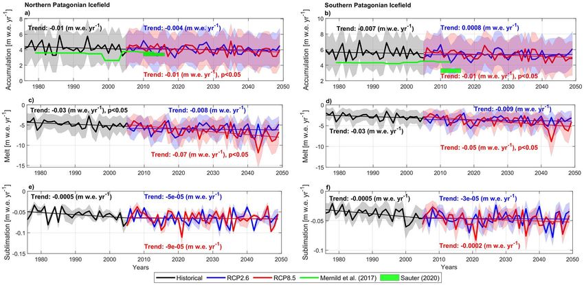
www.nature.com/scientificreports/
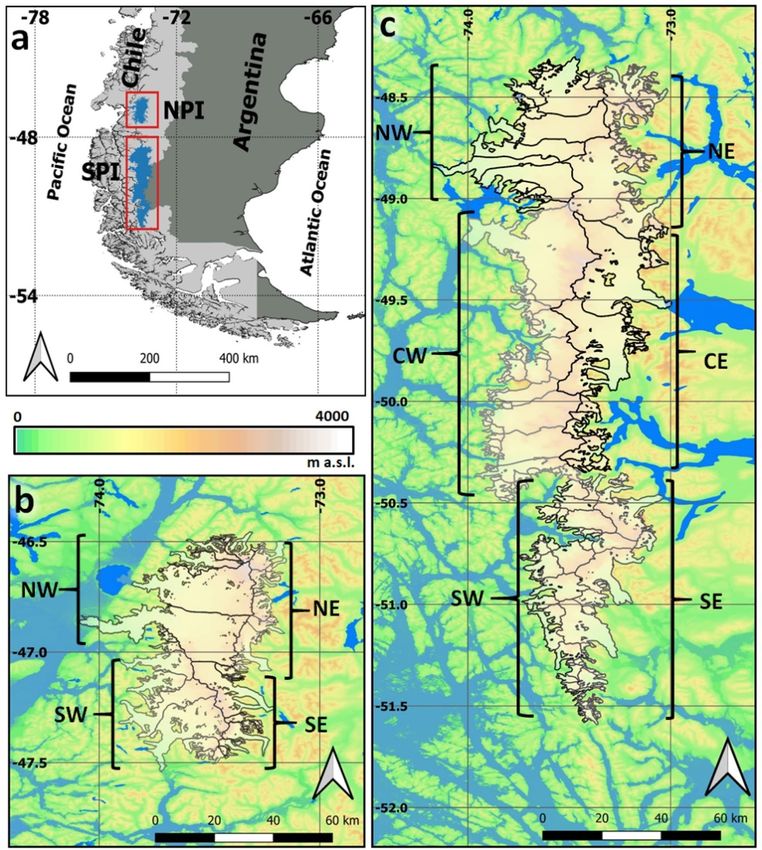
Figure 1. Location of the NPI and SPI in Southern South America (a). Details of the NPI (b) and the SPI (c).
Colour shading is the topography from SRTM at 90 m spatial resolution and blue tones are lakes and fjords. In
the NPI the main glaciers per each sub-zone are: San Rafael and San Quintin (NW), Exploradores, Soler and
Nef (NE), Steffen and Acodado (SW) and Colonia, Pared Norte and Pared Sur (SE). In the SPI: Jorge Montt,
Témpano, Bernardo, Occidental and Greve (NW), O’Higgins and Chico (NE), Pio XI, HPS12, HPS13, Europa
and Guilardi (CW), Viedma and Upsala(CE), Calvo, Asia and Amalia (SW) and Perito Moreno, Grey and
Tyndall (SE). Maps (a–c) were made using QGIS 3.12 București (www.qgis.org).
important, but turbulent fluxes are high in Patagonia, which in turn depend on wind speed, humidity gradients
and near-surface air temperature, among o thers28,29. Secondly, feedbacks between ice dynamics and SMB have
been identified for the glaciers in this region. Patagonian glaciers comprise temperate i ce30 leading to the pres-
ence of abundant meltwater, enhancing crevassing in the terminus areas and leading to flotation and increasing
frontal ablation31. Additionally, a strong correlation between ice speed and air temperature fluctuations has been
evidenced for the calving terminus of the Perito Moreno Glacier in the SPI32,33, suggesting that the meltwater
infiltrating into the glacier increases basal water pressure, which in turn increases basal sliding and thus overall
ice speed.
In view of the local, regional and worldwide impacts observed due to the ongoing glacier shirnkage of Patago-
nian glaciers, and the direct and indirect importance of the climate conditions that drive the total ice loss, an
assessment of the potential future SMB is both critical and timely. The aim of this work is therefore to estimate
Scientific Reports | (2021) 11:16847 | https://doi.org/10.1038/s41598-021-95725-w 2
Vol:.(1234567890)
www.nature.com/scientificreports/
Figure 2. Time series of the modelled surface annual mass balance. (a) NPI and (b) SPI. Colour shadow
represent the uncertainties in the modelled SMB for the historical period and the two scenarios. This shadow
area is due to the parametrization of the glacier cooling effect and the method used for the phase partitioning in
the total precipitation to define the surface snow accumulation. Green coloured bars indicate previously derived
geodetic mass balances and their error range previously estimated in N PI3,4,6,8–12 and in the S PI3,5,7,9–12. Trends
with the 95% confidence interval are shown. Significant trends are also indicated when p < 0.05.
the SMB and its components, including the surface ablation, accumulation and sublimation for both the NPI
and the SPI (Fig. 1) until the year 2050.
We used dynamically downscaled outputs of the MPI-ESM-MR Earth System Model34 obtained with Regional
Model RegCM4.6 at 10-km spatial resolution and daily time step for the historical p eriod35 (hydrological years
April–March between 1976/77 and 2004/05) and for two Representative Concentration Pathways (RCP2.6 and
RCP8.5, between hydrological years 2005/06 and 2049/50). The choice of the MPI-ESM-MR Earth System
Model was made because it is one of the best available for representing the large-scale climate characteristics of
the Southeast Pacific35. RCPs were chosen to best represent current emissions (RCP8.5)36, and to best represent
temperature targets as laid out by the 2015 Paris Agreement (RCP2.6)37. These products were used directly
to estimate snow accumulation and its changes, and subsequently to feed an energy balance model (EBM) to
estimate the ablation and its changes over both Patagonian Icefields. Changes in the equilibrium-line altitudes
(ELA) obtained from the SMB were also analysed and first-order estimations of the ice loss and its associated
contribution to sea-level rise until 2050 were derived.
This approach represents a first assessment of the potential future response of the Patagonian Icefields glaciers
using daily data until 2050. The focus here is to assess how these icefields are responding to ongoing climate
change and what their trajectories will be given future climate scenarios. In the first section of this manuscript, we
compare the results of the historical SMB run with previous estimations of modelled and geodetic mass balance,
as well as the ELA, at the scale of the two icefields. Then, we present the results of the future SMB and ELA under
both scenarios and we quantify the changes in comparison to the historical period as well as estimating total
ice loss. Finally, we discuss the implications of the results in terms of potential glacier response and feedbacks
associated with changes in ELA, SMB and their components.
Results
Historical SMB and ELA. For the historical period, the mean SMB was negative in the NPI, reaching an
annual mean value of − 0.6 ± 2.1 m w.e. yr−1, in agreement with previously published geodetic mass balances in
comparable periods3,4,6,8–12 (Fig. 2a, Table S2) and with previously modelled SMBs (e.g. mean of − 0.2 ± 0.7 m
w.e. yr−1 for the period 1979/80–2009/1023). One previous s tudy26 suggested a slightly positive modelled SMB
of 0.2 ± 0.5 m w.e. y r−1 for the period 1979/80–2013/14, but this is not inconsistent with our computation given
the relative large uncertainty. This can be partly explained by noting that the periods of analysis are not directly
comparable in each case. For the common period between the hydrological years of 1979/80 and 2003/04, we
obtained an annual mean of − 0.7 ± 2.1 m w.e. y r−1 while Mernild et al.26 estimated 0.1 ± 0.5 m w.e. y r−1. Addi-
tionally, we note that all previous values are in the uncertainty range estimated for our historical SMB, which is
higher than previous assessments and reflects the uncertainty mainly associated with snow accumulation and
the parametrization of the glacier cooling effect (see Data and Methods section).
In the SPI (Fig. 2b), SMB was positive with a mean of 2.7 ± 1.6 m w.e. y r−1 during the historical period, in
agreement with the positive SMB computed by previous modelling studies, although our results exceed those of
1.8 ± 0.4 m w.e. yr−126 and 2.3 ± 0.9 m w.e. yr−125 between 1979/80 and 2009/10. For the hydrological years between
1979/80 and 2003/04 we obtained 2.7 ± 1.6 yr−1 m w.e. and Mernild et al.26 derived a value of 1.7 ± 0.4 yr−1 m w.e.
Geodetic mass balances were all negative3,5,7,9–12 and outside of our uncertainty range (Fig. 2b, Table S3). There
was a slightly decreasing trend during the historical period in the SMB which was not significant, but which
contradicts previous SMBs for a similar period that showed a positive t rend24,25.
Scientific Reports | (2021) 11:16847 | https://doi.org/10.1038/s41598-021-95725-w 3
Vol.:(0123456789)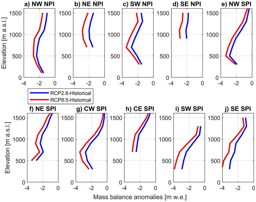
www.nature.com/scientificreports/
Aniya38 (Direct
observation 1983– This work for Rivera et al.4 This work for Barcaza et al.39 This work for Schaefer et al.23
1986 and aerial the same years of (ASTER 10/ the same year of (Landsat between the same years of (SMB modelling This work
a) NPI photographs) Aniya38 Feb/2002) Rivera et al.4 1979 and 2003) Barcaza et al.39 1975–2011) 1975–2005
NW 1031 849 ± 201 1019 756 ± 176 949 ± 41 835 ± 207 1185 ± 6 792 ± 187
NE 1217 1491 ± 107 1224 1446 ± 156 1371 ± 154 1462 ± 136 1387 ± 4 1433 ± 155
SW 1044 990 ± 117 1026 968 ± 145 924 ± 192 1018 ± 147 1163 ± 6 971 ± 134
SE 1075 1415 ± 66 1138 1407 ± 77 1124 ± 101 1414 ± 68 1351 ± 7 1396 ± 86
De Angelis39 (MODIS Feb. 2002 and This work for the same years De Schaefer et al.25 (SMB modelling
b) SPI Feb. and March 2004) Angelis39 1975–2011) This work 1975–2005
NW 928 ± 44 728 ± 93 1112 684 ± 98
NE 1164 ± 38 1335 ± 171 1282 1232 ± 247
CW 1017 ± 53 703 ± 100 989 669 ± 92
CE 1248 ± 55 1410 ± 127 1249 1351 ± 153
SW 1042 ± 62 656 ± 80 900 632 ± 72
SE 1018 ± 28 1103 ± 118 1023 1048 ± 152
Table 1. Comparison of the ELA per sub-zone obtained in this work for the historical period with those
obtained by observations of the end of summer snowline using satellite images4,38–40 and by SMB modelling23,25.
Previous values are the mean of several glaciers observed. Number of glaciers are variable depending
availability in the references. The uncertainty range in our work is given by the sensitivity of the model to the
parametrization of the cooling effects and the methods used to compute the partitioning of rain and snow.
The mean long-term ELA was estimated for the historical period for each sub-zone defined in Fig. 1. Overall,
the west side showed a lower ELA in comparison to the east side glaciers for both icefields. Although there are
no previous estimations that can be directly compared with our ELAs (as most of them are for particular years),
observing the end-of-summer snowline using satellite i mages4,5,38–40 provides some form of validation (Table 1).
Our modelled values compared to those observed in particular years, tend to overestimate the ELA in the eastern
side of both icefields, and notable differences are found along the western margins, where our ELA was generally
100–300 m lower than previous estimations depending on the parameterization (e.g. cooling effect).
A disagreement between the end-of-summer snowline and the mean long-term ELA along the western
margins is likely to reflect the high mass turnover observed in maritime glaciers. In addition, snow accumula-
tion events also occurs in summer m onths19, but a high post-event 0 °C isotherm means much of this snow is
39
quickly lost to m
elt . Additionally, high uncertainty in the snow accumulation rates could lead to a high uncer-
tainty of our modelled ELA. The underestimation in ELA values compared to end-of-summer snowlines suggests
that overestimation in the snow accumulation rate could be the main cause of this discrepancy.
Projected changes in SMB and ELAs. Projected SMB results (which as stated do not account for fron-
tal ablation mechanisms) indicate that the NPI will be characterized by a notable negative SMB until at least
2050. Solely driven by climate forcing, the SPI will continue to gain mass but with lower values compared to
the historical period (Fig. 2). In the NPI, the mean projected SMB values were − 2.0 ± 2.5 m w.e. yr−1 (RCP2.6)
and − 2.5 ± 2.6 m w.e. yr−1 (RCP8.5), while in the SPI, the projected mean SMB values were 1.6 ± 2.0 m w.e. y r−1
(RCP2.6) and 1.3 ± 2.1 m w.e. y r−1 (RCP8.5). However, after the year 2040, a predominance of negative annual
SMB in the SPI is projected.
There are notable differences in the interannual variability in the SMB between RCPs. For instance, some
particular years from the RCP2.6 scenario were lower in magnitude than those arising from the RCP8.5 SMB
run, indicating that the EBM used here seems to capture feedbacks related to other meteorological variables
used to feed the model. This is important as it has been demonstrated that the surface ablation of the Patagon-
ux28,29, which in turn also
ian glaciers depends to a large extent on turbulent fluxes, especially the sensible heat fl
depends on the wind speed. However, the natural interdecadal variability also could play a role in this behaviour,
especially over the first decades of the projection. After 2040, the differences between both scenarios are greater
as the higher signal-to-noise ratio for the RCP8.5 scenario dominates (as it has a more prominent temperature
increase). As might be expected, long-term mean values show that RCP8.5 yielded the greatest reductions in
SMB for both icefields.
Figure 3 shows the projected mean SMB differences compared to the historical period per elevation range, for
each RCPs and for the different sub-zones defined for both icefields (Fig. 1). The reductions in SMB were homo-
geneous within different regions, but with some differences in the magnitude between regions, being notably
larger in the lower section of the south of the SPI (Fig. 3i,j) and lower in the higher elevations (i.e. plateau zone)
of the north-central section of the SPI (Fig. 3e,f,g,h). Due to the RegCM4.6 resolution, the higher zones at each
icefield (> ~ 1500 m a.s.l.) are not represented well (see Fig. S1).
From the SMB profiles (see the Equilibrium-Line Altitude Methods section), we estimated the mean long-
term ELA for each sub-zone and the two pathway scenarios (2005/06–2949-50). Depending on the scenario
and the SMB uncertainties, the magnitude of the ELA increase compared to the historical period could reach
118 ± 42 m in the NPI, while in the SPI could reach a maximum of 94 ± 73 m (Table 2).
Scientific Reports | (2021) 11:16847 | https://doi.org/10.1038/s41598-021-95725-w 4
Vol:.(1234567890)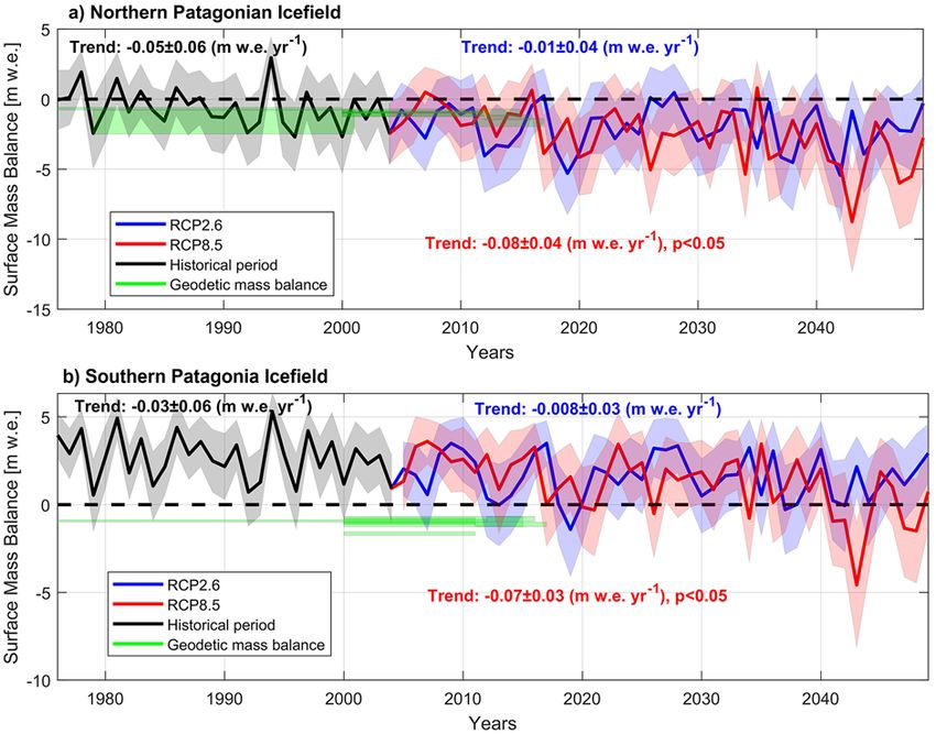
www.nature.com/scientificreports/
Figure 3. Surface mass balance differences per sub-zone (Fig. 1) and elevation range in both icefields. The
differences were derived by comparing long-term SMBs between the historical period and each RCP scenario.
Annual time series and trends in accumulation, melt and sublimation. Annual time series of the
components of the SMB are given in Fig. 4. We found that the variance of the annual SMB depends largely on
the ablation (R2 0.88 and 0.94 for the NPI and SPI, respectively) rather than accumulation (R2 of 0.57 and 0.73,
respectively).
Almost all the components in each scenario and during the historical period show trends that lead to negative
SMB in the NPI and lower, but still positive, SMB in the SPI (Fig. 2). Surface accumulation in the NPI (Fig. 4a)
showed an overall decrease for the historical period and both scenarios, being marginally statistically significant
(p < 0.05) in the RCP8.5 scenario. SPI accumulation (Fig. 4b) showed a slight decrease during the historical
period and RCP8.5 scenario and a slight increase for RCP2.6. Previous estimations of the snow accumulation
trend for both icefields also showed a non-significant change at annual scale for the period 1980–2015; however
a significant increase in snow accumulation during the autumn season was found for the same p eriod19.
In the case of surface melt, an overall increase was determined over the historical period and both scenarios
and for both icefields. The projected melt increase was statistically significant (p < 0.05) during the historical
period in NPI (Fig. 4c) and for scenario RCP8.5 in both icefields. The magnitude of the change was larger
in the NPI compared to SPI (Fig. 4d). Notably, the surface melt projected for the hydrological year 2043/44,
reaches ~ 12 m w.e. yr−1 in NPI and ~ 9 m w.e. y r−1 in SPI. When excluding this large value, the trends were still
significant at 0.008 m w.e. yr−1. Finally, sublimation showed an increase during the historical period and then
plateaus during both future scenarios for both icefields, although its contribution to overall ablation is negligible
according to our results.
Ice loss and contribution to sea‑level rise. In this section, we estimate the ice loss and the contribution
to sea-level rise to year 2050 for both Patagonian Icefields. We make a key assumption that future rates of frontal
ablation will be unchanged from those estimated during past and present conditions, masking the interannual
variability as has been estimated, for instance, in Jorge Montt Glacier31. We calculate these frontal ablation rates
by differencing our modelled SMB and previously published geodetic mass b alances3–12 (Tables S2 and S3). Since
the RCP simulations start in 2005, we used the mean SMB of the two scenarios in order to compare with the
geodetic mass balances calculated after this year. For the NPI, for the period 1975–2016 (Table S2), we derive
a mean frontal ablation contribution of 0.2 ± 0.9 m w.e. y r−1; for the SPI and between 1975 and 2016, the mean
difference was 3.3 ± 0.8 m w.e. yr−1.
In terms of mass, for the NPI, we derive a total frontal ablation of 2.4 ± 3.6 Gt yr−1 in accordance with the
robust estimation by Minowa et al.41 which estimated 2.5 ± 0.5 Gt yr−1. For the SPI, the estimated frontal ablation
was 45.9 ± 15.9 Gt y r−1. This latter value is larger than the 40.7 Gt y r−1 estimated between 1975 and 2000 for the
SPI, but lower than the 56.2 Gt y r−1 obtained between 2000 and 2 01125. The frontal ablation estimation by Minowa
et al.41 in the SPI reaches 21.6 ± 1.7 Gt yr−1, which is far lower than our estimation and previous ones. To match
this value, the SMB in the SPI must decrease ~ 1.5 m w.e. Introducing this correction we obtained a mean SMB
Scientific Reports | (2021) 11:16847 | https://doi.org/10.1038/s41598-021-95725-w 5
Vol.:(0123456789)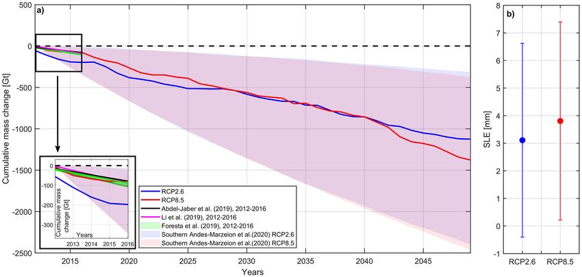
www.nature.com/scientificreports/
Icefield Sub-zone RCP2.6 RCP8.5
NW 92 ± 35 118 ± 42
NE 49 ± 39 62 ± 50
NPI
SW 70 ± 24 86 ± 29
SE 26 ± 36 30 ± 40
NW 49 ± 9 66 ± 16
NE 82 ± 65 94 ± 73
CW 45 ± 18 58 ± 21
SPI
CE 49 ± 31 55 ± 31
SW 36 ± 10 49 ± 15
SE 57 ± 22 69 ± 25
Table 2. Range of difference in the mean long-term ELA per sub-zone between historical period and each
RCP scenario. ELA was obtained as the long-term mean of the elevation where the SMB reached 0 m w.e.
The range of difference at each scenario is given by the runs using − 1 °C and − 3 °C of cooling effect as
meteorological observations suggests18 as well as the uncertainty given by the different methods used to the
partitioning between rain and snow19.
Figure 4. Annual values (hydrological years 1976/77–2049/50) and linear trends of the SMB components in m
w.e. in NPI and SPI for the historical period and the two RCPs. (a,c,e) are accumulation, melt and sublimation in
the NPI and (b,d,f) are accumulation, melt and sublimation in the SPI. Trends with the 95% confidence interval
are shown. Significant trends are also indicated when p < 0.05. Trends in melt for RCP2.6 are significant where
estimated between 1976 and 2050, reaching 0.03 ± 0.01 m w.e. in NPI and 0.02 ± 0.009 m w.e. in SPI.
of 1.2 ± 1.6 m w.e. y r−1 for the historical period, while the projections changes to mean values of 0.1 ± 1.9 m w.e.
yr−1 (RCP2.6) and − 0.3 ± 2.1 m w.e. yr−1 (RCP8.5).
Estimation of total ice mass loss between 2012 and 2050 and total sea-level rise equivalent to the year 2050 is
shown in Fig. 5. Between 2012 and 2030 the greatest reduction in SMB is associated with the RCP2.6 scenario,
after which the largest ice mass loss is projected by RCP8.5, particularly after 2040. RCP8.5 results agree well
with those of Abdel-Jaber et al.12, Foresta et al.9 and Li et al.42 (Fig. 5) between 2012 and 2016, particularly so in
the NPI where frontal ablation (and specifically calving) plays only a minor role. Our ice loss estimates are in the
range of those shown by Marzeion et al.43 (Fig. 5), but it is worth noting that their results incorporate the entire
Southern Andes, and with the exception of one model, neglect frontal ablation mechanisms entirely.
The total equivalent sea-level rise estimated here for both icefields, aggregated between 2012 and 2050
(Fig. 5b) reaches 3.1 mm (RCP2.6) and 3.8 mm (RCP8.5). Within this, the SPI contributes the largest part with
2.3 and 2.8 mm, respectively. The uncertainty, however, is large mainly due to the lack of knowledge in defining
the actual range of the snow accumulation rate, which we introduce in our SMB modelling (Fig. 4a,b).
Scientific Reports | (2021) 11:16847 | https://doi.org/10.1038/s41598-021-95725-w 6
Vol:.(1234567890)www.nature.com/scientificreports/
Figure 5. Cumulative ice loss estimated for both icefields combined between 2012 and 2050 (a) and total
equivalent sea-level contribution to year 2050 (b). For comparison purposes, data from Marzeion et al.43 is
showed (grey area). Marzeion et al.43 ice mass loss corresponds to all the models runs under scenarios RCP2.6
and RCP8.5 computed for the Southern Andes RGI region. Ice mass loss estimations by Abdel-Jaber et al.12,
Foresta et al.9 and Li et al.42 for the four first years (2012–2016) are also shown. Inset, corresponds to a detailed
view of this period.
Discussion
The results of our modelling showed that the surface melt increase during the period 1975–2050 is the main
driver that leads to a reduction in the SMB in both Icefields. For the NPI, a negative SMB will prevails well into
future decades. For the SPI, a correction was introduced in order to reconcile the SMB model results with the geo-
detic mass balances and the independent estimate of the frontal a blation41. In this case, mean SMB projected for
the period 2005–2050, was barely positive (RCP2.6) or negative (RCP8.5). Moreover, a rise in the ELA throughout
both icefields was projected. These changes agree with projected warming in the region (Fig. S2) and align with
previous observations of the high sensitivity of Patagonian glaciers to ablation and air temperature v ariations14.
Qualitatively, an agreement between the surface and geodetic mass balance in the NPI seems to be related to
the frontal characteristics of the glaciers. Many of them are located on land and terminate in small lakes, reducing
the effect of frontal ablation. It has been estimated that calving flux was insignificant for the San Quintin Glacier,
the largest glacier in the NPI, during the period 1975–200023. The exception is San Rafael Glacier, which termi-
nates in a lake connected to a fjord, where previous studies have defined the frontal ablation as being the most
important ice loss mechanism44 being one order of magnitude higher than for most of the NPI glaciers23. Most
glaciers in the SPI are tidewater-terminating in the west and freshwater-terminating in the east. Both fjords and
lakes are of considerable depth, indicating frontal ablation plays an important role31. Nonetheless, the difficulties
in the quantification of the frontal ablation lead to more simple assumptions, and thus, we assumed a constant
value for the projections. As mentioned, Minowa et al.41 estimated a lower frontal ablation rate, which if we
assume for the recent past and future conditions, generates a reduction in our SMB of 1.5 m w.e. This reduction
is in the SMB uncertainty range (Fig. 2) and could be associated mainly with the high uncertainty in defining
the actual snow accumulation (Fig. 4b). Indeed, the mean snow accumulation rate at the SPI after the correction,
would be close to those previously estimated by S auter15 who state that climate models tend to overestimate the
precipitation in Patagonia. In case of implementing a single high-resolution regional climate model driven by a
single global climate model, such biases can be amplified by combined sources of biases and uncertainties due to
boundary conditions and regional climate model itself. In this respect, RegCM4.6 at 10 km resolution tends to
overestimate the annual precipitation over the Andes cordillera in Patagonia if compared with gridded products
derived from observations35. This overestimation is largely associated with the inherited errors from the bound-
ary conditions as well as from the RegCM4.6 itself (e.g. physical configuration), and transferred to our snow
accumulation estimate, which eventually leading to a high uncertainty, depending on the used method (Fig. 4b).
The overestimation of the snow accumulation could be spatially concentrated on the western side, especially on
the SPI, where lower ELA values were obtained in comparison to end-of summer snowline for particular years.
Introducing the correction after the frontal ablation computed by Minowa et al.41, a rise in the ELA between 50
and 100 m was estimated, approaching the values previously observed (Table 1) although differences persist.
The overall reduction of the SMB projected for the next decades, will lead to a continuation or acceleration of
the impacts associated with glacier shrinkage as has been observed in recent decades in the region, and also to
an increase in the contribution to sea-level rise. Other than the positive or barely negative SMB that is projected
for the SPI, a rise in ELA was projected for the NPI. The extent to which this impacts glacier length depends
on several factors, including h ypsometry40 and bed slope45. Previous work has shown that glaciers with a lower
bed slope (e.g. San Quintin Glacier in NPI where negative SMB and ELA rise has been computed) could retreat
Scientific Reports | (2021) 11:16847 | https://doi.org/10.1038/s41598-021-95725-w 7
Vol.:(0123456789)www.nature.com/scientificreports/
around 50 m for each m of ELA r ise45. This means that even without accounting for dynamic changes and mass
loss via calving, some glaciers could retreat between 3 and 8 km within the next 30 years. It should be noted,
however, that the projected rise in ELA in areas of the SPI could occur under the positive mass balance, meaning
that glacier retreat in these zones solely associated with climate forcing will not occur. Potential glacier retreat will
introduce new changes in the landscape. For instance, subglacial topography estimates suggest that pro-glacial
lakes will likely form in several new areas of both the SPI and NPI46. These changes will in turn affect calving rates
and subsequently glacier dynamics, making the prediction of future glacier evolution very complex23. Our estima-
tion in this sense is, therefore, best considered first order. Actually, it is possible that in some areas frontal ablation
rates could reduce as the glaciers thin, or even retreat out of their lacustrine or marine environments and onto
land23. This scenario has already been proposed for the future evolution of Jorge Montt Glacier in the SPI; if the
ongoing retreat continues, the glacier front will stabilise above the fjord level, reducing frontal ablation o verall31.
Evidence found in the Patagonian Icefields, however, seems to suggest further positive feedbacks related
to the increases in surface melt, and associated dynamic adjustments in calving glaciers32 and the appearance
of supraglacial melt p onds17, which would serve to decrease the local surface albedo. Several s tudies32,44 have
evidenced acceleration of glaciers in response to an increase of the basal sliding due to an input of meltwater
percolating to the base. The temperate conditions of the ablation zones of Patagonian glaciers mean that refreez-
ing would be minimal, and the subglacial hydrological network will likely play an important role in determining
future dynamic behaviour. Under this assumption, glacier mass change could be not responding directly to the
SMB change, but instead, it would depend importantly on one of the components of the SMB: the ablation and
specifically the melt, whose increase due to higher air temperature, leads to a larger meltwater input to the glacier
system. This hypothesis could explain in part the overall negative mass change detected in the SPI, while the
SMB is positive or close to balance conditions.
Since glacier dynamics are closely connected to the climate conditions that define the input of meltwater to
the system32,33, a qualitative projection and assessment of glacier response are possible with our results. The areas
with the greatest projected positive trends in the surface melt, in addition to a strong thinning due to surface pro-
cesses, are most likely to be affected by ice acceleration and increases in the calving fl ux27 and frontal a blation33.
These areas are primarily located in the NE of the NPI (e.g. Steffen Glacier), along the western margin of the
SPI (Occidental, Témpano, HPS-29 glaciers) and in the south of the SPI (Tyndall, HPS-38 glaciers) (Fig. 6). To a
lesser extent, a future increase in surface melt was also estimated for the Upsala and Viedma glaciers in the SPI
and San Quintin Glacier in the NPI (Fig. 6). In accordance with our results, most of these Patagonian glaciers
are already thinning rapidly7–9,12. The only exception is Jorge Montt Glacier, located in the SPI. Here, along with
other factors, glacier melt is also forced by warm water entering the fjord, explaining the strong r etreat31 that is
not suggested in our modelled increase in the surface melt (Fig. 6).
In terms of sea-level contribution, the total contribution projected to 2050 for both Icefields, represents a
volume reduction between 22% (RCP2.6) and 27% (RCP8.5) if we compared it with the total sea-level equivalent
of 14.1 mm estimated for both icefields46. The annual rates projected for both icefields are larger than those previ-
ously estimated from the LIA and most of the twentieth century (Table S4). For the 38 years period between 2012
and 2050, we estimated a mean annual rate of both scenarios of 0.067 mm yr−1 for the SPI and 0.024 mm yr−1 for
the NPI, which in total represent 0.091 mm yr−1 for both icefields. These rates are larger than those estimated by
Glasser et al.13 who estimated 0.0018 mm yr−1 between 1870 and 2010 in NPI and 0.005 mm yr−1 between 1750
and 2010 in SPI. Between 1945 and 199647, the contribution of both icefields was estimated to be 0.032 mm yr−1
and between 1968/75–20003 it was estimated as 0.042 mm yr−1. The rate of ice loss during most of the twenti-
eth century is one order of magnitude higher than in previous c enturies13. Additionally, in the last 6 years of
the twentieth century, a new acceleration in ice mass loss was estimated3 reaching a sea-level contribution of
0.105 mm yr−1, while between 2002 and 200647 the sea-level contribution of both icefields was estimated as
0.078 mm yr−1. Therefore, our projected sea-level contribution suggests that accelerated ice loss estimated for
the end of 2 0th3 and the beginning of the 21st42,48 (see Table S4) centuries, will continue under both scenarios.
Conclusions
In this work, we have quantified the present and future SMB for both the NPI and SPI using historical data and
two Representative Concentration Pathways (RCP2.6 and RCP8.5) obtained from the RegCM4.6 model. Snow
accumulation and ablation using an EBM were estimated, as well as their changes throughout the years. We esti-
mated a reduction in the SMB for both icefields. For the NPI a mean reduction between 1.5 and 1.9 m w.e. was
projected for the scenarios RCP2.6 and RCP8.5 respectively, while in SPI the reduction was within the range of
1.1 and 1.5 m w.e. Results of the modelled SMB and ELA in the SPI, suggests an overestimation of the accumu-
lation estimated with the data from RegCM4.6. Overestimation of total precipitation in climate models for the
Patagonia region has also been demonstrated in previous w orks15,28. The independent and robust computation of
41
frontal ablation allowed correction of the modelled SMB for the SPI. Despite an overall reduction in SMB for
the SPI, it was still projected to be positive (RCP2.6) or barely negative (RCP8.5) depending on the RCP. With the
assumption that the annual rate of frontal ablation will remain unchanged, we estimated the contribution of the
ice loss of the Patagonian Icefields to sea-level rise between 2012 and 2050, reaching between 3.1 mm (RCP2.6)
and 3.8 mm (RCP8.5). The projected ELA rise indicates potential area reductions in the glaciers of the NPI as
well as in some areas of the SPI, but limited to those with projected negative mass balances such as in the SW
and only under the RCP8.5 scenario. The magnitude of ELA rise is spatially variable (between 26 and 118 m) and
the impact at each glacier will depend on its topographic characteristics. The trend towards lower SMB overall is
explained by an increase in surface melt and to a lesser extent by a reduction in snow accumulation. The input of
infiltrating meltwater could act as a positive feedback not accounted for in our modelling, triggering ice-speed
acceleration and ice loss due to an increase in frontal ablation of calving glaciers.
Scientific Reports | (2021) 11:16847 | https://doi.org/10.1038/s41598-021-95725-w 8
Vol:.(1234567890)www.nature.com/scientificreports/
Figure 6. Spatially distributed melt trends over the Patagonian Icefields estimated with the EBM. Trends are
from hydrological year 1976/77 to 2049/50, following after 2005 the pathway scenario RCP 2.6 (a) and the
pathway scenario RCP8.5 (b). Black lines are the glacier basins and grey lines are coast lines. All the grid points
are significant (p < 0.05).
Although a complete quantification of future response depends on factors not accounted for by our model-
ling (e.g. ice dynamics), this knowledge of changes owing to climatic conditions gives new insights into recent
trends of ice loss, their controls and uncertainties, and their likely impact on the future response of Patagonian
glaciers through both space and time.
Data and methods
RegCM4.6 simulations. Regional Climate Model, version 4 (RegCM4.6) is a primitive equation and lim-
ited area model developed by the International Centre for Theoretical P hysics49. The dynamical core of the
RegCM4.6 is based on the hydrostatic version of the Penn State/NCAR mesoscale model MM550. RegCM4.6
was used to downscale lateral boundary conditions derived from MPI-ESM-MR Earth System M odel34 on a
nested domain centralizing over Chile at 10-km spatial resolution for historical period (1976–2005) and projec-
tions (2006–2050) under the RCP2.6 and RCP8.5 scenarios35. This study makes use of daily mean near-surface
temperature, total precipitation, wind speed, surface pressure, near-surface relative humidity, incoming short-
wave and longwave radiation obtained from the downscaled RegCM4.6 simulations. RegCM4.6 simulations
used in the present study are based on the land surface model Biosphere–Atmosphere Transfer Scheme of Dick-
inson et al.51 and the radiative scheme of the NCAR Community Climate System Model Version 3 (CCSM3)52.
More information about the simulations, the performance of the RegCM4.6 as well as added value analysis are
detailed in Bozkurt et al.35. Bozkurt et al.35 showed that high-resolution hindcast simulations (i.e. RegCM4.6
forced with reanalysis) robustly simulated the spatiotemporal variability of temperature and precipitation in
southern Chile including the Patagonian Icefields, despite some discrepancies such as the overestimation of
precipitation extremes. In addition, it was also highlighted that coarse resolution boundary conditions can miss
important climate gradients imposed by complex topography in Chile. In this regard, downscaled simulations of
RegCM4.6 forced with MPI-ESM-MR were found to exhibit an added value for both temperature and precipita-
tion by resolving local-scale features in a large part of Chile, including grid points in the Patagonian Icefields.
Nonetheless, there still exist some persistent uncertainties in the RegCM4.6 forced with MPI-ESM-MR such as
Scientific Reports | (2021) 11:16847 | https://doi.org/10.1038/s41598-021-95725-w 9
Vol.:(0123456789)www.nature.com/scientificreports/
precipitation overestimation over the Andes cordillera in Patagonia. In terms of the hypsometry, the topography
of RegCM4.6 (interpolated from GTOPO30) represents quite well the lower elevations and the plateau zone,
although underestimation in the higher elevations is evident compared with the Shuttle Radar Topography Mis-
sion (SRTM) at 1 km resolution (Fig. S1). The areas better represented by the RegCM4.6 topography are between
65 to 70% of the total area in each icefield. Over ~ 1500 m a.s.l. the representation is not good as a clear underes-
timation of the elevation exists. In terms of melt, a minimal impact is expected considering that most of the melt
occurs at lower elevations, but some underestimation of the sublimation is likely.
Surface mass balance. A surface mass balance (SMB) was computed for both icefields. The components
of the SMB were surface melt, sublimation and accumulation and were estimated for each RegCM4.6 grid point
that intersects the icefields. Glacier wide-surface mass balance and its components correspond to the mean
values of each icefield. Even though the resolution of the input data is coarse (~ 10 km), we showed some results
distributed by sub-zones defined in Fig. 1. Considering the resolution of the RegCM4.6 as well as the SMB, the
results are more representative of the large glaciers. More high resolution modelling studies combining both
dynamical and statistical downscaling/bias-correction techniques might be useful to overcome local-scale biases
that are associated with the complex topography.
Ablation: energy balance modelling. A distributed energy balance model (EBM) was applied using
daily data obtained from the RegCM4.6 regional model between 1 April 1976 and 31 March 2050, the Southern
hemisphere mid-latitudes hydrological year. The details of the equations are given in the Supplementary Material
and correspond to the bulk method to estimate sensible, latent and rainfall fluxes including stability corrections
in the first two fluxes. In addition to the meteorological data obtained from RegCM4.6 (previous section), we
estimated additional variables necessary to feed the EBM. These are surface temperature, air and surface vapour
pressure, outgoing longwave radiation, surface albedo and surface roughness. The first three variables, were esti-
mated with standard equations and parametrization and using the data from RegCM4.6. Details of these equa-
tions and parametrization are given in the Supplementary Material. Outgoing longwave radiation was in turn
estimated using the distributed field of the surface temperature and assuming a surface emissivity equal to 1 in
the Stefan-Boltzmann law. The surface albedo was estimated following Oerlemans and K napp53. Surface rough-
ness was estimated using the surface albedo values as a proxy. Here, albedo values between 0.35 to 0.60 were
associated with ice and firn (higher surface roughness) and between 0.60 to 0.80 to different snow ages (lower
surface roughness). From the EBM we obtained the melt and the sublimation at the daily time step, which is then
calculated at the annual time step. The use of daily data allows a better representation of the inter-daily variability
of the albedo and the impact in the reflected shortwave radiation. In order to quantify the uncertainty in one of
the parametrizations, we run two experiments using different magnitudes of the glacier cooling effect assuming
− 1 °C and − 3 °C, respectively. These values were taken from the analysis of air temperature data observed on-
glacier and compared with data measured off-glacier at both sides of the S PI18. Although there are other inherent
uncertainties in the modelling that are hard to quantify, such as the parametrization of the surface roughness,
the use of an EBM makes it possible to integrate more meteorological variables than a temperature-index model
allowing a more complete evaluation of the impacts of the projected climate change over glaciated areas.
Snow accumulation. We estimated the snow accumulation over the glacier surface following the method
of Weidemann et al.28 and Schaefer et al.23,25 previously applied at single glaciers and at the Patagonian Icefield
scale, respectively. This method showed the closest magnitude representation compared with short-term snow
accumulation in the SPI19. We repeat this exercise using the RegCM4.6 data from each RCP. This is presented
in Figure S3, where a clear overestimation is detected using the RCP8.5 data, while RCP2.6 shows also an over-
estimation along the period but a total accumulation close to the estimated accumulation derived from the
ultrasonic-depth gauge (UDG). The source of the overestimation seems to be related to the climate model (MPI-
ESM-MR Earth System Model) used to forced RegCM4.6 due to the fact that snow accumulation estimates
of RegCM4.6 forced by ERA-Interim show a range of value closest to the observed by the UDG in a previous
study19. However, as the uncertainty in precipitation is high15 and hence also in the snow accumulation, we
quantify the uncertainty based on different methods to estimate the partitioning between rain and snow. These
methods are described in full in Bravo et al.19. The input for these estimations was total precipitation, air tem-
perature and relative humidity to estimate dew point temperature for one of the methods19. The daily snow
accumulation was then used to estimate annual accumulation at each hydrological year.
Equilibrium‑line altitude. Equilibrium-line altitudes (ELA) by zone (Fig. 1b,c) were estimated using the
mean value of the specific SMB by elevation range and for each hydrological year. The ELA was then estimated at
the elevation where the annual SMB was equal to 0 m.w.e. In order to compare with previous ELA estimations,
annual values for some years were extracted (Table 1), while the differences between the historical period and
each RCP was estimated based on the long-term mean value.
Ice loss estimation and contribution to sea‑level rise. The ice loss and contribution to sea-level rise
were estimated using previous area and volume data. For the first case, we assume as initial condition the area
estimated for the 2011 year by Davies and G lasser54 and the total volume estimated by Millan et al.55 which was
computed using airborne gravity and radar measurements taken between 2012 and 2016 and complemented
with ice thickness, modelled by Carrivick et al.46. The areas used were 13,219 k m2 for the SPI and 3976 k m2 for
the NPI. Volumes were 3632 k m3 in the SPI and 1124 k m3 in the NPI. Using these data, we estimated the fac-
tors for a bulk volume-area scaling at each icefield. For glacier area S the volume V was estimated as V = cSγ56.
Scientific Reports | (2021) 11:16847 | https://doi.org/10.1038/s41598-021-95725-w 10
Vol:.(1234567890)www.nature.com/scientificreports/
The empirical factor c was estimated, finding that the best adjustment was obtained with c equal to 0.01264 in
NPI and 0.007825 in SPI. The exponent parameter γ is constant and its value is 1.375. The main assumption to
estimate total ice loss in the future was that the annual rate of frontal ablation in the SPI is equal to the present
conditions. The rate of present frontal ablation was estimated following Schaefer et al.25 and assumed that the
differences between geodetic mass balance and modelled SMB correspond to the frontal ablation. In our case,
we estimate the mean of the differences of the values as shown in Tables S2 and S3.
Using the initial conditions, the modelled SMB plus frontal ablation (in the case of the SPI) and the volume-
area scaling parameters, the volume loss at the yearly time step was estimated ( V y ) and consecutively added to
the volume of the previous year (Vy ). The new volume, and using the defined parameters (c and γ) in turn is used
to estimate the new area for the following year ( Ay+1, which is then multiplied with the SMB). This relationship
takes the following form56:
1
Vy + �V y γ
Ay+1 =
c
The volume loss is then adjusted by the area in each time step. Finally, volume is converted to mass using an
ice density of 900 kg m−3, and the resulting ice loss (Gt) is converted to sea-level equivalent.
Received: 15 February 2021; Accepted: 26 July 2021
References
1. Bamber, J. L., Westaway, R. M., Marzeion, B. & Wouters, B. The land ice contribution to sea level during the satellite era. Environ.
Res. Lett. 13, 063008 (2018).
2. Zemp, M. et al. Global glacier mass changes and their contributions to sea-level rise from 1961 to 2016. Nature 568, 382–386
(2019).
3. Rignot, E., Rivera, A. & Casassa, G. Contribution of the patagonia icefields of south America to sea level rise. Science 302(5644),
434–436 (2003).
4. Rivera, A., Benham, T., Casassa, G., Bamber, J. & Dowdeswell, J. Ice elevation and areal changes of glaciers from the Northern
Patagonia Icefield Chile. Glob. Planet. Change 59, 126–137 (2007).
5. Willis, M. J., Melkonian, A. K., Pritchard, M. E. & Rivera, A. Ice loss from the Southern Patagonian Ice Field, South America,
between 2000 and 2012. Geophys. Res. Lett. 39(17), L17501. https://doi.org/10.1029/2012GL053136 (2012).
6. Willis, M. J., Melkonian, A. K., Pritchard, M. E. & Ramage, J. M. Ice loss rates at the Northern Patagonian Ice Field derived using
a decade of satellite remote sensing. Remote Sens. Environ. 117, 184–198 (2012).
7. Malz, P. et al. Elevation and mass changes of the southern patagonia icefield derived from TanDEM-X and SRTM data. Remote
Sens. 10(2), 188 (2018).
8. Dussaillant, I., Berthier, E. & Brun, F. Geodetic mass balance of the Northern Patagonian Icefield from 2000 to 2012 using two
independent methods. Front. Earth Sci. 6, 8. https://doi.org/10.3389/feart.2018.00008 (2018).
9. Foresta, L. et al. Heterogeneous and rapid ice loss over the Patagonian Ice Fields revealed by CryoSat-2 swath radar altimetry.
Remote Sens. Environ. 211, 441–455 (2018).
10. Braun, M. H. et al. Constraining glacier elevation and mass changes in South America. Nat. Clim. Change 9, 130–136 (2019).
11. Dussaillant, I. et al. Two decades of glacier mass loss along the Andes. Nat. Geosci. 12, 802–808 (2019).
12. Abdel-Jaber, W., Rott, H., Floricioiu, D., Wuite, J. & Miranda, N. Heterogeneous spatial and temporal pattern of surface elevation
change and mass balance of the Patagonian ice fields between 2000 and 2016. Cryosphere 13(9), 2511–2535 (2019).
13. Glasser, N. F., Harrison, S., Jansson, K. N., Anderson, K. & Cowley, A. Global sea-level contribution from the Patagonian icefields
since the little ice age maximum. Nature Geosci. 4, 303–307 (2011).
14. Sagredo, E. & Lowell, T. Climatology of Andean glaciers: A framework to understand glacier response to climate change. Global
Planet. Change 86–87, 101–109 (2012).
15. Sauter, T. Revisiting extreme precipitation amounts over southern South America and implications for the Patagonian Icefields.
Hydrol. Earth Syst. Sci. 24, 2003–2016 (2020).
16. Garreaud, R., Lopez, P., Minvielle, M. & Rojas, M. Large-scale control on the Patagonian climate. J. Clim. 26(1), 215–230 (2013).
17. Lo Vecchio, A. et al. MODIS Image-derived ice surface temperature assessment in the Southern Patagonian icefield. Prog. Phys.
Geogr. 43(6), 754–776 (2019).
18. Bravo, C. et al. Air temperature characteristics, distribution and impact on modeled ablation for the South Patagonia Icefield. J.
Geophys. Res. Atmos. 124(2), 907–925 (2019).
19. Bravo, C. et al. Assessing snow accumulation patterns and changes on the Patagonian Icefields. Front. Environ. Sci. 7, 30. https://
doi.org/10.3389/fenvs.2019.00030 (2019).
20. Temme, F., Turton, J. V., Mölg, T. & Sauter, T. Flow regimes and Föhn types characterize the local climate of Southern Patagonia.
Atmosphere 11, 899 (2020).
21. De Angelis, H., Rau, F. & Skvarca, P. Snow zonation on Hielo Patagónico Sur, southern Patagonia, derived from Landsat 5 TM
data. Global Planet. Change 59, 149–158 (2007).
22. Monahan, P. & Ramage, J. AMSR-E melt patterns on the Southern Patagonian icefield. J. Glaciol. 56(198), 699–708 (2010).
23. Schaefer, M., Machguth, H., Falvey, M. & Casassa, G. Modeling past and future surface mass balance of the Northern Patagonian
Icefield. J. Geophys. Res. Earth 118, 571–588 (2013).
24. Lenaerts, J. T. M. et al. Extreme precipitations and climate gradients in Patagonia revealed by high-resolution regional atmospheric
climate modeling. J. Clim. 27(12), 4607–4621 (2014).
25. Schaefer, M., Machguth, H., Falvey, M., Casassa, G. & Rignot, E. Quantifying mass balance processes on the Southern Patagonia
Icefield. Cryosphere 9(1), 25–35 (2015).
26. Mernild, S. H., Liston, G. E., Hiemstra, C. A. & Wilson, R. The andes Cordillera part III: Glacier surface mass balance and contri-
bution to sea level rise (1979–2014). Int. J. Climatol. 37(7), 3154–3317 (2017).
27. Muto, M. & Furuya, M. Surface velocities and ice-front positions of eight major glaciers in the southern Patagonian ice field, South
America, from 2002 to 2011. Remote Sens. Environ. 139, 50–59 (2013).
28. Weidemann, S. S. et al. Glacier mass changes of lake-terminating Grey and Tyndall glaciers at the Southern Patagonia Icefield
derived from geodetic observations and energy and mass balance modeling. Front. Earth Sci. 6, 81. https://doi.org/10.3389/feart
2018.00081 (2018).
Scientific Reports | (2021) 11:16847 | https://doi.org/10.1038/s41598-021-95725-w 11
Vol.:(0123456789)www.nature.com/scientificreports/
29. Schaefer, M., Fonseca, D., Farias-Barahona, D. & Casassa, G. Surface energy fluxes on Chilean glaciers: Measurements and models.
Cryosphere 14, 2545–2565 (2020).
30. Warren, C. R. & Sugden, D. E. The Patagonian icefields: A glaciological review. Arct. Alp. Res. 25(4), 316–331 (1993).
31. Bown, F. et al. Recent ice dynamics and mass balance of Jorge Montt Glacier, Southern Patagonia Icefield. J. Glaciol. 65(253),
732–744 (2019).
32. Sugiyama, S. et al. Ice speed of a calving glacier modulated by small fluctuations in basal water pressure. Nat. Geosci. 4, 597–600
(2011).
33. Minowa, M., Sugiyama, S., Sakakibara, D. & Skvarca, P. Seasonal variations in ice-front position controlled by frontal Ablation at
Glaciar Perito Moreno, the Southern Patagonia icefield. Front. Earth Sci. 5, 1. https://doi.org/10.3389/feart.2017.00001 (2017).
34. Giorgetta, M. A. et al. Climate and carbon cycle changes from 1850 to 2100 in MPI-ESM simulations for the coupled model
intercomparison Project phase 5. J. Adv. Model Earth Syst. 5(3), 572–597 (2013).
35. Bozkurt, D. et al. Dynamical downscaling over the complex terrain of southwest South America: Present climate conditions and
added value analysis. Clim. Dyn. 53, 6745–6767 (2019).
36. Schwalm, C. R., Glendon, S. & Duffy, P. B. RCP8.5 tracks cumulative CO2 emissions. Proc. Natl. Acad. Sci. U.S.A. 117, 19656–19657
(2020).
37. Sanderson, B., Tebaldi, C. & O’Neill, B. What would it take to achieve the Paris temperature targets?. Geophys. Res. Lett. 43,
7133–7142 (2016).
38. Aniya, M. Glacier inventory for the Northern Patagonia Icefield, Chile, and variations 1944/45 to 1985/86. Arct. Alp. Res. 20,
179–187 (1988).
39. Barcaza, G., Aniya, M., Matsumoto, T. & Aoki, T. Satellite-derived equilibrium lines in Northern Patagonia Icefield, Chile, and
their implications to glacier variations. Arct. Antarct. Alp. Res. 41, 174–182 (2009).
40. De Angelis, H. Hypsometry and sensitivity of the mass balance to change in equilibrium-line altitude: The case of the Southern
Patagonia Icefield. J. Glaciol. 60(219), 14–28 (2014).
41. Minowa, M., Schaefer, M., Sugiyama, S., Sakakibara, D. & Skvarca, P. Frontal ablation and mass loss of the Patagonian icefields.
Earth Planet Sc. Lett. 561, 116811 (2021).
42. Li, J., Chen, J., Ni, S., Tang, L. & Hu, X. Long-term and inter-annual mass changes of patagonia ice field from GRACE. Geod.
Geodyn. 10, 100–109 (2019).
43. Marzeion, B. et al. Partitioning the uncertainty of ensemble projections of global glacier mass change. Earth’s Fut. 8, 2 (2020).
44. Collao-Barrios, G., Gilliet-Chaulet, F., Favier, V., Casassa, G. & Berthier, E. Ice flow modelling to constrain the surface mass balance
and ice discharge of San Rafael Glacier Northern Patagonia Icefield. J. Glaciol. 64(246), 568–582 (2018).
45. Oerlemans, J. Linear modeling of glacier fluctuations. Geografiska Ann. Ser. A Phys. Geogra. 94(2), 183–194 (2012).
46. Carrivick, J. L., Davies, B. J., James, W. H. M., Quincey, D. J. & Glasser, N. F. Distributed ice thickness and glacier volume in southern
South America. Global Planet. Change 146, 122–132 (2016).
47. Rivera, A., Acuna, C., Casassa, G. & Bown, F. Use of remotely sensed and field data to estimate the contribution of Chilean glaciers
to eustatic sea-level rise. Ann. Glaciol. 34, 367–372 (2002).
48. Chen, J. L., Wilson, C. R., Tapley, B. D., Blankenship, D. D. & Ivins, E. R. Patagonia Icefield melting observed by gravity recovery
and climate experiment (GRACE). Geophys. Res. Lett. 34, L22501 (2007).
49. Giorgi, F. et al. RegCM4: Model description and preliminary tests over multiple CORDEX domains. Clim. Res. 52, 7–29 (2012).
50. Grell, G. A., Dudhia, J., & Stauffer, D. R. Description of the fifth generation Penn State/NCAR Mesoscale Model (MM5) (NCAR
Tech. Note NCAR/TN-398+STR). Boulder, CO: NCAR (1994).
51. Dickinson, R. E., Henderson-Sellers, A., & Kennedy, P. J. Biosphere-Atmosphere Transfer Scheme (BATS) Version 1e as Coupled
to the NCAR Community Climate Model. NCAR Tech. Note NCAR/TN-387+STR, NCAR, Boulder (1993).
52. Kiehl, J. T. et al. Description of the NCAR Community Climate Model (CCM3) (NCAR Tech. Note NCAR/TN-420+STR). Boulder,
CO: NCAR (1996).
53. Oerlemans, J. & Knap, W. H. A one-year record of global radiation and albedo from the ablation zone of the Morteratschgletscher
Switzerland. J. Glaciol. 44(147), 231–238 (1998).
54. Davies, B. J. & Glasser, N. F. Accelerating shrinkage of Patagonian glaciers from the Little Ice Age (~AD 1870) to 2011. J. Glaciol.
58(212), 1063–1084 (2012).
55. Millan, R. et al. Ice thickness and bed elevation of the Northern and Southern Patagonian Icefields. Geophys. Res. Lett. 46(12),
6626–6635 (2019).
56. Moller, M. & Schneider, C. Calibration of glacier volume–area relations from surface extent fluctuations and application to future
glacier change. J. Glaciol. 56(195), 33–40 (2010).
Acknowledgements
C.B. acknowledge the support from the National Agency for Research and Development (ANID), Scholarship
Program, Doctorado Becas Chile, 2016 – 72170022 and thanks to CECs for the support to finish this manu-
script. D.B. acknowledges support from ANID-CONICYT-PAI 77190080, ANID-FONDECYT-11200101 and
ANID-PIA-Anillo INACH ACT192057. Powered@NLHPC: This research was supported by the supercomputing
infrastructure of the NLHPC (ECM-02).
Author contributions
C.B. designed the study, analysed the data, prepare figures and wrote the Manuscript. D.B. performed the
RegCM4.6 simulations, contributed to the writing, discussed the results and reviewed the manuscript. D.J.Q.
and A.N.R., collaborated with the design, contributed to the writing and oversaw the research.
Competing interests
The authors declare no competing interests.
Additional information
Supplementary Information The online version contains supplementary material available at https://doi.org/
10.1038/s41598-021-95725-w.
Correspondence and requests for materials should be addressed to C.B.
Reprints and permissions information is available at www.nature.com/reprints.
Publisher’s note Springer Nature remains neutral with regard to jurisdictional claims in published maps and
institutional affiliations.
Scientific Reports | (2021) 11:16847 | https://doi.org/10.1038/s41598-021-95725-w 12
Vol:.(1234567890)You can also read