Emulating climate extreme indices - Environmental Research Letters - IOPscience
←
→
Page content transcription
If your browser does not render page correctly, please read the page content below
Environmental Research Letters

LETTER • OPEN ACCESS

Emulating climate extreme indices
To cite this article: C Tebaldi et al 2020 Environ. Res. Lett. 15 074006

View the article online for updates and enhancements.

                                This content was downloaded from IP address 46.4.80.155 on 30/10/2020 at 23:23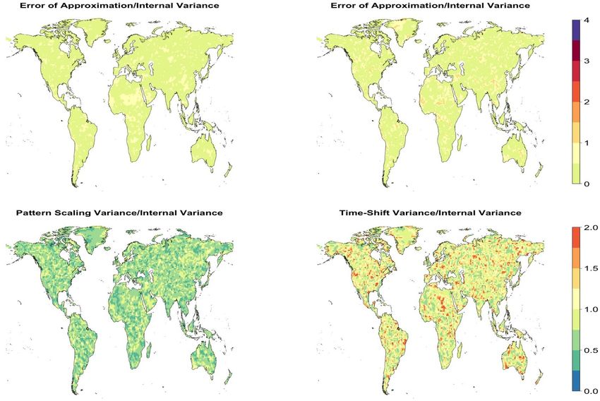
Environ. Res. Lett. 15 (2020) 074006 https://doi.org/10.1088/1748-9326/ab8332
Environmental Research Letters
LETTER
Emulating climate extreme indices
OPEN ACCESS
C Tebaldi1, A Armbruster2, H P Engler2 and R Link1
RECEIVED 1
19 November 2019 Joint Global Change Research Institute, College Park, MD, United States of America
2
Georgetown University, Washington, DC, United States of America
REVISED
13 March 2020 E-mail: claudia.tebaldi@pnnl.gov
ACCEPTED FOR PUBLICATION
Keywords: extreme indices, emulation, scenarios, pattern scaling, time shift, internal variability, error metric
25 March 2020
PUBLISHED
Supplementary material for this article is available online
18 June 2020
Original Content from Abstract
this work may be used
under the terms of the We use simple pattern scaling and time-shift to emulate changes in a set of climate extreme indices
Creative Commons
Attribution 4.0 licence.
under future scenarios, and we evaluate the emulators’ accuracy. We propose an error metric that
Any further distribution separates systematic emulation errors from discrepancies between emulated and target values due
of this work must to internal variability, taking advantage of the availability of climate model simulations in the form
maintain attribution to
the author(s) and the title of initial condition ensembles. We compute the error metric at grid-point scale, and we show
of the work, journal
citation and DOI. geographically resolved results, or aggregate them as global averages. We use a range of scenarios
spanning global temperature increases by the end of the century of 1.5 C and 2.0 C compared to a
pre-industrial baseline, and two higher trajectories, RCP4.5 and RCP8.5. With this suite of
scenarios we can test the effects on the error of the size of the temperature gap between emulation
origin and target scenarios.
We find that in the emulation of most indices the dominant source of discrepancy is internal
variability. For at least one index, however, counting exceedances of a high temperature threshold,
significant portions of the globally aggregated discrepancy and its regional pattern originate from
the systematic emulation error. The metric also highlights a fundamental difference in the two
methods related to the simulation of internal variability, which is significantly resized by simple
pattern scaling. This aspect needs to be considered when using these methods in applications
where preserving variability for uncertainty quantification is important.
We propose our metric as a diagnostic tool, facilitating the formulation of scientific hypotheses
on the reasons for the error. In the meantime, we show that for many impact relevant indices these
two well established emulation techniques perform accurately when measured against internal
variability, establishing the fundamental condition for using them to represent climate drivers in
impact modeling.
1. Introduction of futures. A heightened attention to the role of addi-
tional sources of uncertainty besides scenarios, i.e.
Simple pattern scaling (pattern scaling from now model structure and internal variability (Knutti et al
on) (Santer et al 1990, Huntingford and Cox 2000, 2010, Hawkins and Sutton 2009, Deser 2012) fur-
Tebaldi and Arblaster 2014, Herger et al 2015, Kravitz ther increases interest in computationally efficient
et al 2017) is widely used to emulate fields of future methods able to explore those uncertainty dimen-
changes in climatic variables under arbitrary forcing sions. Ideally these capabilities can be soft- or hard-
scenarios. Output from general circulation models coupled to impact models to robustly characterize
(GCMs) is used to train the emulator, using global risk, and even develop modeling frameworks where
mean temperature change as predictor variable. Since feedbacks between earth and human systems can be
global mean temperature can be efficiently simulated represented. At the same time, the role of extreme
by simple climate models, emulators can explore a events and their future changes in causing signific-
wider range of scenarios than those available from ant impacts makes the development of emulators of
GCM runs, a capability that proves valuable in char- extreme behavior a priority and with it the need for
acterizing impacts of climate change for a broad range rigorous performance evaluation.
© 2020 The Author(s). Published by IOP Publishing Ltd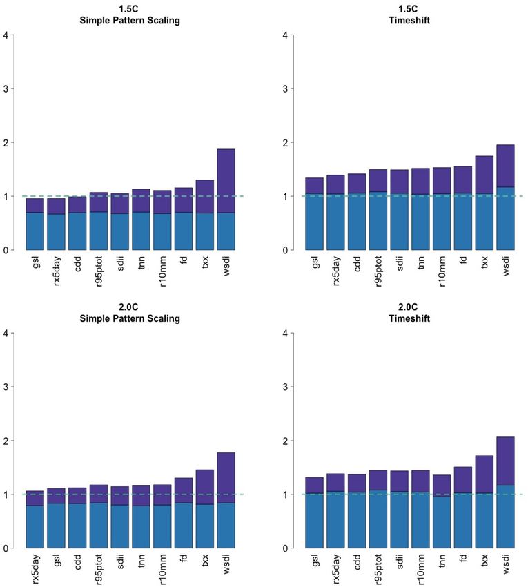
Environ. Res. Lett. 15 (2020) 074006                                                                  C Tebaldi et al

     Several recent studies and assessments                produces more accurate emulations for temperature
(Lustenberger et al 2014, Seneviratne et al 2016,          than for precipitation, but that the uncertainty in
Wartenburger et al 2017, Masson-Delmotte et al 2018)       emulations of both is significantly smaller than the
have shown that not only average temperature and           disagreement over the patterns among models. The
precipitation, but also many indices of extremes           same result was confirmed by Tebaldi and Knutti
appear to change in direct, often linear relation to       (2018) in the context of the emulation of highly mitig-
global drivers (exp. global mean temperature) sup-         ated scenarios. This study extends the analysis beyond
porting the idea of building emulators for extremes        average temperature and precipitation to ten climate
driven by simple models like MAGICC (Meinshausen           extreme indices, using initial condition uncertainty
et al 2011) or Hector (Hartin et al 2015) (which           as benchmark for accuracy, rather than inter-model
through SCENGEN (Wigley 2008) and fldgen (Link             variability. We note that inter-model variability for
et al 2019) respectively already implement pattern         long-term changes is known to dominate internal
scaling for average temperature and precipitation).        variability (Hawkins and Sutton 2009), therefore a
Our aim in this paper is to consider pattern scal-         method found accurate when measured against the
ing and an alternative approach, time-shift (also          latter is also accurate against the former.
known as time-sampling) (James et al 2017, King                 The paper is structured as follows. Section 2
et al 2018, Herger et al 2015), and evaluate their per-    describes the CESM ensembles and their char-
formance in approximating a set of extreme indices.        acteristics, the ten ETCCDI indices and our
Both methods have been previously validated for            error metric. Since the two emulation methods
average quantities (e.g. Tebaldi and Arblaster 2014,       are well established and documented, we only
Kravitz et al 2017, Tebaldi and Knutti 2018) under         briefly introduce them here, and we describe
increasing and stabilized scenarios, showing that the      them in detail in the supplementary material
error introduced by the approximation is of compar-        (stacks.iop.org/ERL/15/074006/mmedia). Section 3
able size to internal variability, and of much smal-       describes the results of the emulations: we give an
ler size than the uncertainty introduced by models’        overview of the performance over the suite of indices,
alternative structural choices (Tebaldi and Knutti         and we then focus on a particular index for which the
2018). Here we use as targets of the emulation ten         globally aggregated error metric and its regional pat-
indices among the Expert Team on Climate Change            terns show a comparatively larger emulation error.
Detection Indices (ETCCDI) suite (Alexander 2016).         We conclude in section 4 by summarizing the validity
We then test the accuracy of the approximations when       of these emulation methods when applied to indices
the origin and target scenarios are relatively closer or   of extremes, pointing at the promise of implementing
farther apart within a range of trajectories that span     these emulators into impact models. We also high-
radiative forcings from less than 2 Wm−2 to approx-        light the value of our metric for uncertainty quan-
imately 8.5 Wm−2 by 2100. We introduce a metric of         tification, in particular the possibility of identifying
emulator error that explicitly separates the portion       regions and processes where linear scaling and time-
that is unavoidable, coming from internal variability      shift fail to perform.
of the target quantity, from the portions that are arti-
facts of the emulation choice, i.e. the internal variab-   2. Data and methods
ility of the emulator output, and the proper emulator
error. We further separate the two latter components,      2.1. Climate model output, scenarios, indices
as only the emulator error needs minimizing. When          NCAR-DOE CESM1-CAM5 (CESM) (Hurrell
this is done at geographically resolved scales, further    et al 2013) was used to simulate historical and future
analysis of the reasons for the emulator performances      climate according to several pathways of future emis-
can be undertaken, zooming into specific regions of        sions, producing ensembles from perturbed initial
the globe and specific processes at play.                  conditions under each of the different scenarios. The
     Explicitly addressing internal variability is made    so called large ensemble (LENS) was documented
possible by the use of a set of initial condition          in Kay et al (2015). It simulates conditions under
ensemble simulations, available for all future scen-       historical and RCP8.5 forcings, with initial con-
arios considered. The actual model output for the tar-     ditions perturbed at 1920. A subsequent project,
get scenario is taken to be the ground truth, against      BRACE (O’Neill and Gettelman 2018), motivated the
which our emulations are validated. A large source of      simulation of an alternative, lower-emission scen-
variability that is not addressed in this study, how-      ario, RCP4.5, for which the first 15 members of the
ever, is model uncertainty, the source of variabil-        historical simulations were used as starting future
ity in model output that derives from each model’s         trajectories at 2005 (Sanderson et al 2018). After
structural choices, as we use ensembles of simula-         the Paris agreements spurred a special report by the
tions from only one GCM. A multi-model ensemble,           IPCC (Masson-Delmotte et al 2018) it was decided to
CMIP5 (Taylor et al 2012), was used in Tebaldi and         produce a further set of three ten-members ensembles
Arblaster (2014), which found that pattern scaling         that reached the 1.5 C and 2.0 C targets at the end of

                                              2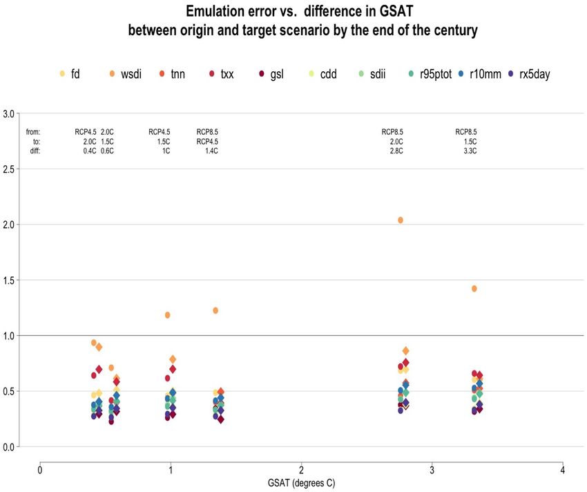
Environ. Res. Lett. 15 (2020) 074006                                                                      C Tebaldi et al

the 21st century (Sanderson et al 2017). For these         In order to approximate lower warming scenario
low-warming scenarios the first ten members of the         A using higher warming scenario B, the method
historical simulations of the LENS were used as start-     identifies a window of a number of years (here we use
ing points at 2005. From the first ten members of all      10) when GSAT from origin scenario B is on average
4 scenarios (1.5 C, 2.0 C, RCP4.5 and RCP8.5) we use       the same as GSAT from the target scenario A. Once
daily output of maximum, minimum and mean tem-             those years from scenario B are isolated, the quantit-
perature (TREFHTMX, TREFHTMN and TREFHT)                   ies of interest are extracted and used straightforwardly
and precipitation (PRECT) to compute ten extreme           as surrogate for the same quantities under scenario A.
indices, which take the form of annual summaries of        We add details about both methods as supplementary
daily weather behavior.                                    material.
    Specifically, we target ten ETCCDI extreme
indices (Alexander 2016). Five indices relate to the       2.3. Error metric
behavior of extreme precipitation: total annual pre-       Our model output consists of ensembles of 10 mem-
cipitation when daily rainfall exceeds the 95th clima-     bers obtained by perturbing initial conditions. We
tological percentile (r95ptot), maximum consecutive        perform the emulation for each of these 10 separ-
five day accumulated precipitation amount (rx5day),        ately, so that we end up comparing 10 emulated fields
annual count of days when precipitation exceeds 10         against 10 ground truth fields for each method. Note
mm (r10mm), average precipitation intensity (sdii)         however that one should not expect a given ensemble
defined as the total precipitation amount during the       member from the target scenario and the correspond-
year divided by the number of wet days (defined in         ing ensemble member from the origin scenario to be
turn as days with at least 1 mm of precipitation),         comparable. This is because the two future traject-
and maximum number of consecutive dry days (i.e.           ories soon become independent of one another due
with precipitation less than 1 mm) (cdd). Five indices     to the short memory of the climate processes at play
relate to the behavior of extreme temperatures: warm       and the difference in forcings immediately after 2005.
spell duration index (wsdi), defined as the longest        We now show how to distinguish internal variability
stretch of days in the year with maximum temperat-         (uncertainty that is present in the climate model out-
ure above the 90th climatological percentile; annual       put, and is thus treated as unavoidable) from system-
number of frost days (fd) when minimum temperat-           atic error, introduced in areas where pattern scaling
ure falls below freezing, growing season length (gsl)      or time-shift are not effective approximation meth-
defined as the period between the last freeze in the       ods. In addition, since the two emulation methods
spring and the first freeze in the fall, minimum tem-      don’t propagate internal variability through the emu-
perature of the coldest day of the year (tnn), and         lation in the same way, we can distinguish the vari-
maximum temperature of the hottest day of the year         ations introduced by the internal variability of the
(txx). The choice of these indices is somewhat arbit-      target data from that represented in the emulated
rary but aims at spanning a wide range of behaviors in     quantities.
temperature and precipitation, more or less extreme               At any grid-point, consider the vectors y =
values, singular events or spells, cold and heat, dry      (y1 , y2 , . . . , yK ) of values from the target (truth)
and wet extremes.                                          ensemble and ŷ = (ŷ1 ,ŷ2 , . . . ,ŷL ) from the emulation
                                                           ensemble. In our case, K = L = 10. As usual we write
2.2. Emulation methods                                     ȳ, ¯ŷ for the ensemble averages of the yi and ŷj . The
We use two different methods for approximating             mean square difference between all possible pairs of
lower warming scenarios from higher ones. The              emulated and true quantities is a measure for their
first one, simple pattern scaling (Santer et al 1990),     closeness. It can be decomposed as follows:
depends upon the assumption that local climate can
                                                              1 X                           2
be modeled as a linear function of Global Surface                 (yi − ŷj )2 = ȳ − ¯ŷ
                                                             KL
Air Temperature (GSAT from now on), where the                      i,j
slope coefficient differs from grid-point to grid-point                            + ⟨(ŷ − ¯ŷ)2 ⟩ + ⟨(y − ȳ)2 ⟩. (1)
but is scenario independent. The field of such coeffi-
cients determines a normalized pattern that is used to          The angle brackets on the right denote averages
provide an approximation of the actual field by mul-       that are computed over one of the two ensembles
                                                                                       P
tiplying by values of GSAT from the target scenario.       each, e.g. ⟨(y − ȳ)2 ⟩ = K1 i (yi − ȳ)2 . A derivation of
We apply the method to each of the ten ensemble            this decomposition is given in the supplementary
members available for any choice of origin-target          material. As pointed out above, this decomposition
scenario, for each of which we obtain one field of coef-   holds at the grid-point level, but we can also think of
ficients. Using each member separately let us explore      it as a vector equation that holds at multiple locations.
the effects of internal variability.                       Only the first term in this decomposition represents
     We also test and compare a second emulation           a true emulation error. The second term is related
method, the time-shift approach (James et al 2017).        to internal variability of the emulated quantity and

                                              3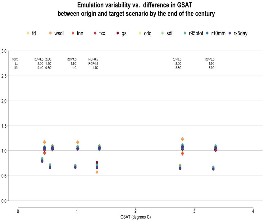
Environ. Res. Lett. 15 (2020) 074006                                                                                           C Tebaldi et al

   Figure 1. Both methods (circles for pattern scaling, diamonds for time-shift) and all indices (color coded according to legend), for
   all pairings of origin and target scenarios (as indicated at the top of the plot): The size of the emulation error scaled by the size of
   the internal variability of the target quantity (first component of our metric (2) is shown as the y-axis dimension. The x-axis
   orders the scenario pairings according to the size of the GSAT gap between them at the end of the century. The metric is first
   computed at each grid-point of the land regions of the globe between 60S and 60 N, then aggregated with weights proportional to
   cosine of latitude.

the third term captures the internal variability of the                 particular it is usually assumed that the closer the ori-
true quantity. We therefore choose to define our error                  gin and target scenarios are, the better the perform-
metric as the two-dimensional quantity                                  ance of the emulation will be, and we will test this
                                 p                !                     assumption here.
                    ȳ − ¯ŷ       ⟨(ŷ − ¯ŷ)2 ⟩
    Er(y,ŷ) = p                ,p                  . (2)
                   ⟨(y − ȳ)2 ⟩    ⟨(y − ȳ)2 ⟩
                                                                        3. Results
This means that we scale the two error components
related to the emulation by the unavoidable variation                   3.1. Globally aggregated metric
of the target quantity.                                                 Figures 1 and 2 summarize our results aggregated at a
    Importantly, the first component of the metric                      global scale (after computing the metric at each grid-
should be as small as possible to reduce system-                        point), separately for each component of the error
atic errors, while the second should be close to 1 to                   metric (2). Each of the symbols in the plot corres-
show that the emulation does not inflate or reduce                      ponds to an index/method combination, with circles
the variability that is in the target ensemble. Both                    referring to pattern scaling results, diamonds refer-
components of the measures become unitless and                          ring to time-shift results. We used warm colors (yel-
we can compare the performance of the emulator                          low to red) for temperature dependent indices and
across quantities with different units, magnitudes,                     cold colors (green to purple-blue) for precipitation-
and variability. This allows one to rank indices with                   dependent indices. For these plots, however, the iden-
respect to the faithfulness of emulation. We will assess                tification of the indices is only aimed at assessing if the
which combinations of origin, target, and emulation                     relative performance of the methods across the index
method produce the most accurate emulations. In                         set remains substantially the same, i.e. the same index

                                                         4
Environ. Res. Lett. 15 (2020) 074006 C Tebaldi et al
Figure 2. As in figure 1, but showing the second component of our metric (2), i.e. the size of the internal variability of the
emulation, scaled by the size of the internal variability of the target. As in figure 1, the metric is first computed at each grid-point
of the land regions of the globe between 60S and 60 N, then aggregated with weights proportional to cosine of latitude.
is found easy (accurately emulated) by both meth- usually at the lower end of the range, likely thanks
ods, or found challenging (poorly emulated) by both to the relatively larger size of the internal variability
methods, and the ranking from easy to challenging of precipitation-based quantities (the denominator in
remains the same across the different origin-target definition (2)). The traditional assessments that find
combinations. We are plotting all the combinations emulating precipitation more challenging than emu-
of origin-target scenarios we have tested as a function lating temperature may therefore be the result of fail-
of the gap in GSAT between the two scenarios at the ing to distinguish discrepancies due to real emulation
end of the century (x-axis), expecting that the smaller error from those due to internal variability. Figure 1
the gap the better the emulation performance. also shows that between the two methods pattern scal-
First, we note that for the large majority of indices ing is always at least equivalent, in most cases bet-
and emulation choices, and for both methods, the ter than time-shift (except for wsdi). Also interest-
value of the emulation error (figure 1, along the ingly, there is no dependency between the size of the
y-axis) is less than one, i.e. is less than the size of emulation errors and the size of the gap in GSAT
internal variability of the true quantity. The only between scenarios. Our study is framed around the
exception is the index wsdi, which quantifies changes comparison of the two emulation methods, and as
in the duration of warm spells. The index appears time-shift cannot approximate higher scenarios, only
to be particularly challenging for pattern scaling sug- the emulation of lower scenarios from higher one can
gesting that the assumption of linearity adopted by be assessed for both. In the supplementary material
pattern scaling is the source of the error. We will we show a similar plot to figure 1 for simple pattern
further explore this behavior in the next subsection. scaling, where we evaluate emulating higher scenarios
As for all other indices, we can assess that indeed by lower ones. The larger magnitude of the errors,
the ranking with respect to difficulty of emulation increasing with the GSAT gap between the origin and
remains substantially constant across methods and target scenarios confirms that it is advisable to emu-
origin/target scenario pairs. Precipitation indices are late down, rather than up. As pattern scaling aims at
5Environ. Res. Lett. 15 (2020) 074006 C Tebaldi et al
Figure 3. Each of the panels correspond to an origin-target scenario pairing and a method, with RCP4.5 used to emulate 1.5 C
(top row) and 2.0 C (bottom row) and pattern scaling results in the left plots, time-shift results in the right plots. Each bar shows
the two error components with lighter blue representing the internal variability of the emulation (that should be optimally close
to 1, marked by the dotted line). The indices (with names along the bottom) are ordered according to the increasing size of the
emulation error portion, measured by the dark purple section of the bars.
estimating the forced signal of change it is to be expec- the higher origin scenario) which dampens the vari-
ted that using a high scenario facilitates its extraction, ability of the patterns. Time-shift does not apply any
making the exercise more robust. rescaling, and, if anything its results suggest a slight
Figure 2 repeats the lay-out of figure 1, but shows overestimation of internal variability, which can be
the second component of the error metric, which due to the use of scenarios with larger emissions to
should be close to 1. Here the two methods show a emulate lower emission targets. Again, in the supple-
consistently different performance, with pattern scal- mentary material we show a similar plot for the res-
ing systematically underestimating, time-shift closely ults of applying pattern scaling to the emulation of
replicating the internal variability of the target. The higher scenarios from lower ones, and again we can
former result can be explained by the definition of assess the larger discrepancies between emulated and
pattern scaling which, by construction, multiplies the true internal variability, in this case by construction
normalized pattern by a constant that is less than one showing higher variability, as a factor greater than one
(the ratio of GSAT for the lower target scenario and is applied.
6Environ. Res. Lett. 15 (2020) 074006 C Tebaldi et al
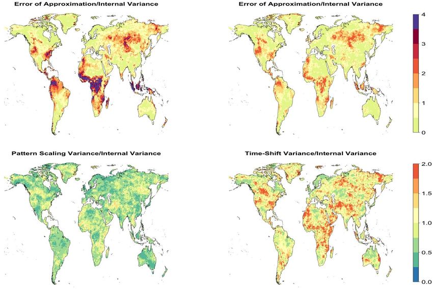
Figure 4. Patterns of the two components of the error metric for the index rx5day, maximum 5-day precipitation amount of the
year. Left column shows results for pattern scaling; right column for time-shift. The top panels show the size of the emulation
error component (a multiple of the internal variability of the target quantity). The bottom panels show the ratio of the emulation
internal variability to the internal variability of the target quantity.
Figure 3 shows the comparison of the two meth- differences in performance to a difference in the way
ods for the emulation of the 1.5 C and 2.0 C tar- the two methods reproduce internal variability.
get scenarios using RCP4.5 as the origin (results Concluding this portion of the assessment we
from other origin-target combinations are available underline that the characteristics of smaller or lar-
as supplementary material) highlighting the relat- ger internal variability in the emulation results are
ive contribution of the two terms of the error met- not necessarily a shortcoming or a benefit, depend-
ric (blue/lighter for the internal variability term, ing on the application. However, since most applica-
purple/darker for the emulation error term, adding tions of emulating extreme indices are likely used in
up to the total error as the height of each bar). A impact models we would expect the representation of
dashed line in each plot marks the unit line. Time- internal variability to be an important component of
shift can be seen replicating a measure of internal any risk assessment.
variability closer to one (from above) than pattern
scaling, whose blue bars are relatively farther from
the unit line (from below). The index wsdi stands 3.2. Geographically resolved metric
out with the larger portion due to emulation error, We now present a disaggregated view of the same res-
which remains for all other indices smaller than one. ults, examining geographical patterns of error. The
Note that more traditional metrics measuring emu- global measures gave us a means to assess the overall
lation performance through root mean square errors emulation performance for the indices, and enabled
(RMSEs) without distinguishing the two compon- a quick comparison among them. A spatial analysis
ents would have used the total height of the bars in can highlight geographic features specific to the vari-
figure 3 without distinguishing the two components ous sources of error and variability, can give insight
of each bar. In that case the message would have been into the causes of inaccuracies, and can help identify
substantially, but we argue deceptively, simpler with those physical processes responsible for the emula-
one of the methods, pattern scaling, clearly a winner tion error. We use two indices showing very different
showing lower RMSEs for all but one index. Having outcomes for the two components of the error met-
decomposed the error metric into a component that ric, rx5day, which measures the wettest 5 consecutive
is the true emulation error and a component due to days of the year, and wsdi, already identified as the
internal variability of the emulation result, we instead index with a large emulation error, which counts the
can interpret the results more subtly, connecting the longest spell in the year of warm days (i.e. days above
7Environ. Res. Lett. 15 (2020) 074006 C Tebaldi et al
Figure 5. As in figure 4, but for the index wsdi, warm spell duration.
the estimated 90th percentile of the climatological poses challenges to the emulation to a significantly
distribution of local temperature). We illustrate the higher degree than the rest of the ETCCDI suite. We
analysis using results from the emulation of the 1.5 C already expected this from the size of the top portion
scenario (the target) based on RCP4.5 (the origin). In of the bars for the index in figure 3, top row (last bar
figure 4 for rx5day and 5 for wsdi we show 4 panels, to the right in both panels) but now we can identify
2 for each method (pattern scaling on the left, time- where the sources of the error are, geographically,
shift on the right), with the first metric component and attempt formulating hypotheses for the causes of
(the emulation error) on the top row, the second (the the errors.
internal variability) on the bottom row. As is indic- The pattern of emulation errors in the top two
ated by the corresponding bars in figure 3 for rx5day panels of figure 5 identifies specific regions of the
(second bar from the left in both top panels), figure 4 subtropics as the sources of the larger discrepan-
shows that both approaches produce a similarly small cies between emulated and true index values. A map
emulation error (significantly less than one when showing Net Primary Productivity of vegetation from
globally aggregated). Consistently with their beha- the land component of CESM would identify many
vior over other indices, pattern scaling estimates too of the same areas as locations where broad-leaf forest
little internal variability, while time-shift reproduces grows (see figure 1 in the supplementary material)
it accurately. Geographically, patterns are consistently and one could be justified in speculating about the
and smoothly below 1 for the emulation error, and differential role of CO2 fertilization effects on vegeta-
noisily below or around 1 for the internal variability tion in the two scenarios (origin and target), possible
component. No feature stands out that raises ques- surface-atmosphere interactions when more or less
tions about regional effects worth investigating, at moisture is available from vegetation transpiration
least at this fairly broad, bird’s eye perspective. In con- and therefore possible effects on precipitation and
trast, the same analysis for wsdi in figure 5 shows that temperature in these regions. This is the type of hypo-
both emulation methods find challenges in similar thesis that could be used as a starting point for sci-
regions, particularly pattern scaling, with values of the entific investigation, further experiments, closer ana-
emulation error well above 1 in large coherent regions lysis of time series and spell behavior. That would
of the subtropics. In lesser measure the same regions be beyond the scope of this work, however, and we
also appear in the error patterns of time-shift. Internal mention it only as an example of the type of analysis
variability is slightly underestimated overall by pat- enabled by the close inspection of the regional beha-
tern scaling, but significantly overestimated in many vior of the error. In the supplementary material we
regions by time-shift. This is definitely an index that elaborate on the source of the error further.
8Environ. Res. Lett. 15 (2020) 074006 C Tebaldi et al
Maps similar to those in figures 4 and 5 for the significantly larger trends in the higher origin scen-
remaining 8 indices are available in the supplement- arios’ windows than in the lower target scenarios,
ary material, from which we can confirm that no likely because the variability of these extreme quant-
emulation error presents itself as starkly as for the ities mutes any trend that may be present in a ten year
index wsdi. Specific applications that focus on lim- window. Along with these effects of internal variabil-
ited regional areas may still find the decomposition ity we noticed that emulation of precipitation indices
eye-opening, and stimulating more in-depth error appears to benefit from the explicit accounting of its
analysis. role: we are used to think of emulation of precipita-
tion as relatively more challenging than that of tem-
perature until we recognize that the larger variabil-
4. Discussion and conclusions ity should provide larger ‘tolerance’ for the emulation
errors. We were also able to make a systematic com-
Two emulation methods, simple pattern scaling and parison of the performance of the emulation methods
time-shift, already well established for the emula- as a function of the distance between origin and tar-
tion of average quantities, are here tested for a set get scenarios, and found that there is no definite gain
of indices of temperature and precipitation extremes. in choosing the closest scenario available to the target,
After introducing a new error metric able to distin- especially within a small range of the gap size (on the
guish true emulation error from discrepancies intro- order of a fraction of a degree) where the differential
duced by internal variability we find that for almost all in performance is not robust.
these indices both methods perform accurately. This
is a promising finding as we aim at representing more,
and more impact relevant, climate drivers in our Acknowledgments
impact models, expanding on recent efforts identify-
ing a broad range of hazards and their indices Mora This work was funded by the U.S. Department of
et al (2018), Forzieri et al (2018). Having tested emu- Energy, Office of Science, as part of research in
lation performance on a broad range of indices we the MultiSector Dynamics, Earth and Environmental
are confident that for most temperature and precipit- System Modeling Program. The Pacific Northwest
ation indices the implementation of their emulation National Laboratory is operated for DOE by Bat-
will be successful, but hazards come from different telle Memorial Institute under contract DE-AC05-
weather and climate variables too, like winds, extreme 76RL01830. The views and opinions expressed in this
sea levels, snow and ice storms etc for which the emu- paper are those of the authors alone. The initial ana-
lation is sure to present new challenges. lyses originate from the summer project of Alex Arm-
Our work is focused on the characteristics of the bruster’s undergraduate internship at the National
error metric as much as on the actual results of the Center for Atmospheric Research. That portion,
emulation exercise: we show that there is value in dis- together with Claudia Tebaldi’s time at NCAR was
tinguishing the true emulation error from the com- supported by the Regional and Global Model Analysis
ponent of the discrepancy due to internal variab- (RGMA) component of the Earth and Environmental
ility generated by the emulator. A traditional view System Modeling Program of the U.S. Department
of emulation error would seek a method that deliv- of Energy’s Office of Biological & Environmental
ers an unbiased estimate (a small emulation error Research (BER) via National Science Foundation IA
term in our metric) and is affected by small variance 1947282.
(a small internal variability term in our metric).
The first requirement is unquestionable and in our Data availability statement
application sees pattern scaling taking a comparat-
ive advantage over time-shift for all but one index. The data that support the findings of this study are
Contrary to the second requirement, for many uses available from the corresponding author upon reas-
of the emulated values an ability to recreate internal onable request.
variability besides average behavior should in fact
be desirable. If we embrace this point of view, the ORCID iDs
comparative advantage is reversed between the meth-
ods: simple pattern scaling shows too small variab- C Tebaldi https://orcid.org/0000-0001-9233-8903
ility while time-shift reproduces in most cases the R Link https://orcid.org/0000-0002-7071-248X
variability of the target. Interestingly the closer ana-
lysis of time-shift internal variability suggests that the
output under the higher scenarios appears in most References
cases not to show significantly different variability
Alexander L V 2016 Global observed long-term changes in
compared to the lower target scenarios at the time
temperature and precipitation extremes: a review of
when global average temperature is similar. That also progress and limitations in ipcc assessments and beyond
suggests that many of these quantities do not show Weather. Clim. Extremes. 11 4–16
9Environ. Res. Lett. 15 (2020) 074006 C Tebaldi et al
Deser C, Phillips A, Bourdette V and Teng H 2012 Uncertainty in Masson-Delmotte V, Zhai P, Portner H, Roberts D, Skea J, Shukla
climate change projections: the role of internal variability P and et al ed 2018 IPCC (2018). Global warming of 1.5C. An
Clim. Dyn. 38 527 IPCC Special Report on the impacts of global warming of 1.5C
Forzieri G, Bianchi A, Batista e Silva F, Marin Herrera M A, above pre-industrial levels and related global greenhouse gas
Leblois A, Lavalle C, Aerts J and Feyen L 2018 Escalating emission pathways, in the context of strengthening the global
impacts of climate extremes on critical infrastructures in response to the threat of climate change, sustainable
europe Glob. Environ. Change 48 97–107 development, and efforts to eradicate poverty (Geneva: World
Hartin C A, Patel P, Schwarber A, Link R P and Bond-Lamberty B Meteorological Organization)
P 2015 A simple object-oriented and open-source model for (www.ipcc.ch/site/assets/uploads/sites/2/2019/06/SR15_Full_
scientific and policy analyses of the global climate system Report_Low_Res.pdf)
hector v1.0 Geosci. Model. Dev. 8 939–55 Meinshausen M, Raper S C B and Wigley T M L 2011 Emulating
Hawkins E and Sutton R 2009 The potential to narrow coupled atmosphere-ocean and carbon cycle models with a
uncertainty in regional climate predictions Bull. Am. simpler model, MAGICC6 part 1: Model description and
Meteorol. Soc. 90 1095–108 calibration Atmos. Chem. Phys. 11 1417–56
Herger N, Sanderson B M and Knutti R 2015 Improved pattern Mora C et al 2018 Broad threat to humanity from cumulative
scaling approaches for the use in climate impact studies climate hazards intensified by greenhouse gas emissions Nat.
Geophys. Res. Lett. 42 3486–94 Clim. Change 8 1062–71
Huntingford C and Cox P M 2000 An analogue model to derive O’Neill B and Gettelman A 2018 An introduction to the special
additional climate change scenarios from existing GCM issue on the benefits of reduced anthropogenic climate
simulations Clim. Dyn. 16 575–86 change (brace) Clim. Change 146 277–85
Hurrell J W, Holland M M and Gent P R 2013 The community Sanderson B M et al 2017 Community climate simulations to
earth system model: A framework for collaborative research assess avoided impacts in 1.5 and 2◦ C futures Earth Syst.
Bull. Am. Meteorol. Soc. 94 1339–60 Dynam. 8 827–47
James R, Washington R, Schleussner C-F, Rogelj J and Conway D Sanderson B, Oleson K W, Strand W G, Lehner F and O’Neill B
2017 Characterizing half-a-degree difference: a review of 2018 A new ensemble of gcm simulations to assess avoided
methods for identifying regional climate responses to global impacts in a climate mitigation scenario Clim. Change
warming targets Wiley Interdiscip. Rev. Clim. Change 8 e457 146 303–18
Kay J E, Deser C, Phillips A, Mai A, Hannay C, Strand G and Santer B D, Wigley T M L, Schlesinger M E, and Mitchell J 1990
Vertenstein M 2015 The community earth system model Developing climate scenarios from equilibrium gcm
(CESM) large ensemble project: A community resource for results Report of the Max Plank Institut f ur Meteorologie
studying climate change in the presence of internal climate 47 29
variability Bull. Am. Meteorol. Soc. 96 1333–49 Seneviratne S I, Donat M G, Pitman A J, Knutti R and Wilby R L
King A D, Knutti R, Uhe P, Mitchell D M, Lewis S C, Arblaster J M 2016 Allowable CO2 emissions based on regional and
and Freychet N 2018 On the linearity of local and regional impact-related climate targets Nature 529 477
◦ ◦
temperature changes from 1.5 C to 2 C of global warming Taylor K E, Stouffer R J and Meehl G A 2012 An overview of
J. Clim. 31 7495–7514 CMIP5 and the experiment design Bull. Am. Meteorol. Soc.
Knutti R, Furrer R, Tebaldi C, Cermak J and Meehl G A 2010 93 485–98
Challenges in combining projections from multiple climate Tebaldi C and Arblaster J M 2014 Pattern scaling, its strengths and
models J. Clim. 23 2739–58 limitations and an update on the latest model simulations
Kravitz B, Lynch C, Hartin C and Bond-Lamberty B 2017 Clim. Change 122 459
Exploring precipitation pattern scaling methodologies and Tebaldi C and Knutti R 2018 Evaluating the accuracy of climate
robustness among cmip5 models Geosci. Model. Dev. change pattern emulation for low warming targets Environ.
10 1889–902 Res. Lett. 13 055006
Link R, Snyder A, Lynch C, Hartin C, Kravitz B and Wartenburger R, Hirschi M, Donat M G, Greve P, Pitman A J
Bond-Lamberty B 2019 Fldgen v1. 0: an emulator with and Seneviratne S I 2017 Changes in regional climate
internal variability and space–time correlation for earth extremes as a function of global mean temperature: an
system models Geosci. Model. Dev. 12 1477–89 interactive plotting framework Geosci. Model. Dev.
Lustenberger A, Knutti R and Fischer E M 2014 Sensitivity of 10 3609–34
european extreme daily temperature return levels to Wigley T M L 2008 MAGICC/SCENGEN 5.3: User manual
projected changes in mean and variance J. Geophys. Res.: (version 2) (Boulder, CO: NCAR) 80 (http:
Atmos. 119 3032–44 //acacia.ucar.edu/cas/wigley/magicc/UserMan5.3.v2.pdf)
10You can also read