The TR-808 Cymbal: a Physically-Informed, Circuit-Bendable, Digital Model - Queen's University Belfast
←
→
Page content transcription
If your browser does not render page correctly, please read the page content below
The TR-808 Cymbal: a Physically-Informed, Circuit-Bendable, Digital
Model
Werner, K. J., Abel, J., & Smith, J. (2014). The TR-808 Cymbal: a Physically-Informed, Circuit-Bendable, Digital
Model. In A. Georgaki, & G. Kouroupetroglou (Eds.), Proceedings of the 40th International Computer Music
Conference and the 11th Sound and Music Computing Conference (pp. 1453–1460).
http://quod.lib.umich.edu/cgi/p/pod/dod-idx/tr-808-cymbal-a-physically-informed-circuit-bendable-
digital.pdf?c=icmc;idno=bbp2372.2014.221
Published in:
Proceedings of the 40th International Computer Music Conference and the 11th Sound and Music Computing
Conference

Document Version:
Publisher's PDF, also known as Version of record

Queen's University Belfast - Research Portal:
Link to publication record in Queen's University Belfast Research Portal

Publisher rights
© 2014 The Author(s).
This is an open access article published under a Creative Commons Attribution License (https://creativecommons.org/licenses/by/3.0/),
which permits unrestricted use, distribution and reproduction in any medium, provided the author and source are cited.

General rights
Copyright for the publications made accessible via the Queen's University Belfast Research Portal is retained by the author(s) and / or other
copyright owners and it is a condition of accessing these publications that users recognise and abide by the legal requirements associated
with these rights.

Take down policy
The Research Portal is Queen's institutional repository that provides access to Queen's research output. Every effort has been made to
ensure that content in the Research Portal does not infringe any person's rights, or applicable UK laws. If you discover content in the
Research Portal that you believe breaches copyright or violates any law, please contact openaccess@qub.ac.uk.

Download date:15. Mar. 2021
Proceedings ICMC|SMC|2014                      14-20 September 2014, Athens, Greece

  The TR-808 Cymbal: a Physically-Informed, Circuit-Bendable, Digital Model

                                           Kurt James Werner, Jonathan S. Abel, Julius O. Smith
                                        Center for Computer Research in Music and Acoustics (CCRMA)
                                                    Stanford University, Stanford, California
                                            [kwerner | abel | jos]@ccrma.stanford.edu

                                ABSTRACT                                                  in music journalism, but this has distracted from focused
                                                                                          study of the individual voice circuits. The 808’s cymbal
We present an analysis of the cymbal voice circuit from a                                 voice circuit represents a significant leap forward in the
classic analog drum machine, the Roland TR-808 Rhythm                                     design of analog drum machine voices—it is a complex,
Composer. A digital model based on this analysis (im-                                     efficient circuit that reasonably approximates a real cym-
plemented in Cycling 74’s Gen˜) retains the salient fea-                                  bal sound.
tures of the original. Developing physical models of the                                     The 808 cymbal has only a few user-controllable param-
device’s many sub-circuits allows for accurate emulation                                  eters: decay, tone, and level. To access the latent potential
of circuit-bent modifications (including component substi-                                of the circuit, drum machine modders add additional tun-
tution, changes to the device’s architecture, and voltage                                 ing and architecture-level controls, even going so far as to
starve)—complicated behavior that is impossible to cap-                                   allow external audio to be routed through the circuit [6].
ture through black-box modeling or structured sampling.                                   This tradition parallels the development of circuit-bending
This analysis will support circuit-based musicological in-                                and other music hardware hacking, and could potentially
quiry into the history of analog drum machines and the de-                                be lost in the process of digitally emulating an 808.
sign of further mods.                                                                        By adopting a physically-informed approach, and favor-
                                                                                          ing an analysis that elucidates the design intent, this work
                         1. INTRODUCTION                                                  supports informed mods of the circuit. A more compli-
                                                                                          cated analysis could obscure the logic of the device’s con-
Despite significant work that has been done on cloning and
                                                                                          struction, with minimal gains in accuracy. Framing the
emulating the TR-808, there is an almost complete lack of
                                                                                          analysis in terms of component values simplifies the sim-
published analyses on the circuit. 1 We have begun to fill
                                                                                          ulation of mods based on component substitution. 3 Parti-
this void with [3], which develops a physically-informed,
                                                                                          tioning the circuit into blocks allows for the simulation of
circuit-bendable, digital model of the TR-808’s bass drum
                                                                                          mods based on changes to the circuit’s architecture. 4
voice circuit. In the following paper, we will use related
                                                                                             We give an overview of the circuit in §2 and an anal-
techniques (well-represented in virtual analog literature) to
                                                                                          ysis of each part of the circuit and their interconnections
analyze the 808’s cymbal voice circuit.
                                                                                          in §§3–11. This is followed by a discussion of modeling
   The goals of this research are to partition the 808’s cym-
                                                                                          techniques in §12 and results in §13.
bal circuit into functional blocks, create a physically-in-
formed analysis of each block, model each block in soft-
ware, and evaluate the results. Throughout, we will pay                                                              2. OVERVIEW
special attention to developing an analysis in terms of the
electrical values of circuit elements.                                                    Fig. 1 shows a schematic diagram of the TR-808 cymbal
   It is particularly important to analyze the 808 in this way,                           circuit. This annotated schematic labels important nodes
because of the extant misinformation surrounding the de-                                  and currents, and shows how the circuit is broken down
vice. 2 The 808’s rich mythology has been well-covered                                    into blocks: Schmitt trigger oscillators (see §3), band pass
                                                                                          filters (see §4), trigger logic (see §5), an attack smoother
   1 previous work includes [2], which offers a qualitative discussion
                                                                                          (see §6), envelope generators (see §7), “swing-type voltage-
of [1] in the context of imitating classic synthesized cymbal voices with
modular synthesizers                                                                      controlled amplifiers” (VCAs, see §8), high pass filters
   2 For instance: the user manual for the Novation Drum Station (an
                                                                                          (see §9), a tone control stage (see §10), and an output buffer
early rack-mount TR-808/TR-909 emulator) says the cymbal sound is
generated by “multiple noise sources,” which is patently false. Some                      and level control (see §11). Fig. 2 shows a block diagram
improbable stories about the machine’s design turn out to be true. Don                    of the digital model of the cymbal circuit. Both figures
Lewis, an early pioneer of drum machine modification, worked on the
design of the 808 and even developed techniques that influenced its voice
design [4]. He relates a story from his visit to Roland’s Tokyo offices in                on inside–he sort of bumped up against the breadboard and spilled some
the late 70s, where he worked with chief engineer Tadao Kikumoto. “That                   tea in there and all of a sudden he turned it on and got this pssh sound–it
day he had a bread board of an 808 and was showing me what was going                      took them months to figure out how to reproduce it, but that ended up be-
                                                                                          ing the crash cymbal in the 808. There was nothing else like it. Nobody
                                                                                          could touch it.” [5]
                                                                                             3 for instance: adding tuning controls to the oscillators, band pass fil-
Copyright: c 2014 K. J. Werner et al. This is an open-access article distributed
                                                                                          ters, and high pass filters; additional controls to the static envelope gener-
under the terms of the Creative Commons Attribution 3.0 Unported License, which           ators; or extending the tone controls.
                                                                                             4 for instance: allowing each of the 6 rectangular wave oscillators or
permits unrestricted use, distribution, and reproduction in any medium, provided
                                                                                          the bands to be individually muted, bypassing filters, or injecting external
the original author and source are credited.                                              audio.

                                                                                   - 1453 -
Proceedings ICMC|SMC|2014 14-20 September 2014, Athens, Greece
Figure 1. TR-808 cymbal schematic (adapted from [1]).
should be consulted alongside the analysis of each block This primarily had the effect of a producing a tunable cow-
in the following sections. bell voice. However, they also form an important part of
To produce a cymbal note, the µPD650C−085 CPU ap- the cymbal sound as well. 7
plies a common trigger and (logic high) instrument data The inverter has only low and high output states (VOL
to the trigger logic. The resulting 1-ms long pulse is de- and VOH ), and transitions between them are subject to hys-
livered to the envelope generators via an attack smoother. teresis. When an input voltage VI rises above a positive-
The output of this smoother drives four envelope signals, going threshold voltage VT + , the output swings to VOL .
which are applied to three swing-type VCAs, where they When VI falls below a negative-going threshold voltage
control the amplitude of three bands of filtered rectangu- VT − , the output swings to VOH . 8
lar wave clusters. Two different active band pass filters Since the positive-going and negative-going threshold
sum and filter the output of six Schmitt trigger inverter os- voltages for a Schmitt trigger input are different, the circuit
cillators, producing these clusters. The output of each of will oscillate back and forth as the capacitor is alternatively
the three swing-type VCAs is applied to a corresponding charged and discharged. Considering the continuous-time
Sallen-Key high pass filter. From there, each band is ap- cases of a charging and discharging capacitor separately
plied to a tone control stage and a level control, which sums yields the capacitor charge and discharge times:
the three bands back together and buffers the output.
VOH − VT −
tcharge = RC · ln (1)
3. SCHMITT TRIGGER OSCILLATORS VOH − VT +
VOL − VT +
The TR-808’s Cowbell, Cymbal, Open Hihat, and Closed tdischarge = RC · ln . (2)
VOL − VT −
Hihat voice circuits all work by filtering and enveloping
rectangular waves. In fact, they all share a common bank These times sum to the total period of oscillation T =
of six of these oscillators, ingeniously implemented with a tcharge + tdischarge . Since the oscillator switches between
single HD14584 hex Schmitt trigger inverter chip. In each output states VOL and VOH , its amplitude is trivially equal
of these astable multivibrators, the Schmitt trigger inverter to their difference. The duty cycle is, by definition, the pro-
acts as the bistable element, and a passive network of a portion of time that the oscillator spends in its high state.
single resistor and capacitor provides an RC time constant Now, the salient features (frequency f = 1/T , amplitude
that tunes the oscillator to a particular frequency. 5 A = VOH − VOL , and duty cycle D = tcharge/T ) are avail-
Oscillators #1–4 are hardwired to a particular frequency.
The last two, which form the basis of the Cowbell voice creators of 808 clones and emulators. See: [7], Tactile Sounds’ TS-808,
Analogue Solutions’ Concussor, Acidlab’s Miami, &c.
circuit, are tunable via trimpots that are only accessible 7 Robin Whittle points to component tolerance (and, by extension,
by opening up the TR-808’s internals. Although this was variations in tuning for oscillators #5–6) as the source of the unique char-
intended for factory tuning, early drum machine hackers acter of individual 808 cymbals [6].
8 The switching characteristics (output rise and fall time, propaga-
were quick to pull these controls out to the front panel. 6 tion delay time [8]) of the HD14584 are all faster than 250 ns, and
5 This technique was well-known to hardware hackers as early as
the transitions are smooth. Keeping in mind the bandwidth of human
hearing (roughly, 20–20,000 hertz, corresponding to a minimum period
the 1960s, and forms an important building block of so-called “Lunetta of 50 µs), this transition is treated as instantaneous. We forego alias-
Synths”—CMOS-based devices inspired by the designs of Stanley suppressed methods for rectangular wave simulation (for instance: [9]),
Lunetta. since the aliased components will be sufficiently filtered out or perceptu-
6 Nowadays, this technique is well-documented among hackers and ally masked downstream.
- 1454 -Proceedings ICMC|SMC|2014 14-20 September 2014, Athens, Greece
Figure 2. TR-808 cymbal emulation block diagram.
able in terms of passive component values and the device amplitude (volts)
0.2 SPICE
properties of the Schmitt trigger inverter. model
0.1
Plugging in Equations (1)–(2) to the definition of duty
cycle, the time constant RC drops out—the duty cycle de- 0
0.07 0.072 0.074 0.076 0.078 0.08
pends only on the inverter’s device properties VT − , VT + , time (seconds)
VOL , and VOH :
Figure 3. Sum of all oscillators (Vsum ).
VOH −V −
(VOH −V − )(VOL −V + )
T
D= ln VOH −V +
T
/ln T T
(VOH −V + )(VOL −V − )
. (3)
T T
4. BAND PASS FILTERS
The six oscillators have nominal frequencies (or ranges)
of 205.3, 369.6, 304.4, 522.7, 359.4–1149.9, and 254.3– The two active band pass filters 13 each filter the combina-
627.2 Hz. Oscillators #5–6 have internal trimpots (TM2 tion of the six rectangular waves. What follows is a rep-
and TM1 ) in series with their resistor, for factory tuning to resentative analysis and simulation of band pass filter #1.
specific frequencies (800 and 540 Hz, respectively). 9 Identical methods were used for #2.
Assuming ideal op-amp behavior, nodal analysis of band
By design, the HD14584 is powered with 5 volts, yield-
pass filter #1 yields a transfer function of the form:
ing a duty cycle of D = 47.98% and an amplitude of
A = 5 volts for each oscillator. 10 Vbp#1 β2 s2 + β1 s
All six oscillators are summed via voltage dividers in Hbp1 (s) = = , (5)
Vsum α3 s + α2 s2 + α1 s + α0
3
a passive mixing network. The output of this network is
applied to the input of the band pass filters. Respecting with coefficients:
superposition (grounding the other oscillator outputs), an
β2 = −R56 R57 (C13 + C14 ) C10
example calculation of this attenuation (for oscillator #1)
β1 = −R57 C10
is:
α3 = R56 R57 R52 C13 C14 C10
Vsum R53 α2 = R56 R57 C13 C14 + R56 R52 (C13 + C14 ) C10
= . (4)
VO,1 R53 + (R37 k R39 k R46 k R48 k R50 ) α1 = R56 C13 + R56 C14 + R52 C10
α0 = 1.
Fig. 3 shows a comparison between the sum of all six os-
cillators (the signal applied to each band pass filter) and Fig. 4 shows the magnitude response of each band pass
tabulated data from a SPICE 11 simulation of the circuit. 12 filter. Band pass filter #1 has a center frequency around
3440 Hz and band pass filter #2 has a center frequency
9 Early manufacturing runs (prior to serial #000300) used different val-
around 7100 Hz. These band pass filters strongly accen-
ues for the resistors and capacitors in oscillators 5 and 6 [1].
10 using the “typical” values from the device’s datasheet [8] tuate the upper overtones of the square waves, while de-
11 Simulation Program with Integrated Circuit Emphasis, a widely- emphasizing their fundamental frequencies.
used family of general purpose analog electronic circuit simulators.
12 No attempt was made to align the phase of the model to the tabu- 13 whose topologies are closely related to the so-called “bridged-T net-
lated SPICE data. Fig. 3 just shows, qualitatively, that the model and the work”, a bridged-T Zobel network in the negative-feedback path of an
reference SPICE simulation have similar features. op-amp, that is used in each of the 808’s voice circuits [3]
- 1455 -Proceedings ICMC|SMC|2014 14-20 September 2014, Athens, Greece
amplitude (volts)
20 Hbp1 6
magnitude (dB)
Hbp2 4 Vtrig
10 Hh1 Vsmooth − SPICE
2
Hh2 Vsmooth − model
0 0
Hh3 1.2 1.4 1.6 1.8 2
time (seconds) −3
−10 x 10
3 4
10 10
frequency (hertz)
Figure 6. Attack smoother output, no accent, time domain.
Figure 4. Magnitude responses of band pass and high pass
filters. ing form approximates the behavior of this circuit:
Vsmooth 1
Has (s) = = , (6)
Vtrig − VBE 1 + τs
where VBE is the voltage drop from the base of Q19 to its
emitter, and τ is an RC time constant. The values of these
constants are found by least-squares minimization to be:
VBE = 0.7258 , τ = 1.0244 · 10−4 .
Fig. 6 shows good agreement between this simplified model
and tabulated data from SPICE.
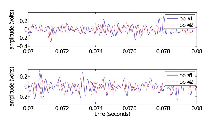
Figure 5. Band pass response in time domain, physical 7. ENVELOPE GENERATORS
model (top) and SPICE (bottom). The attack smoother applies a smoothed trigger Vsmooth
to three envelope generators via D6 –D8 . These envelopes
serve as amplitude control for each swing-type VCA. What
Fig. 5 shows typical behavior in the time domain. Each
follows is a representative analysis and simulation of enve-
time one of the six rectangular wave oscillators flips state,
lope generator #1. Identical methods were used for #2–3.
the edge kicks some more AC energy into each band pass
In envelope generator #1, an emitter follower buffers the
filter.
first stage (EG #1.1). The output of the emitter follower
drives two more stages (EG #1.2 and EG #1.3).
5. TRIGGER LOGIC The first stage EG #1.1 is comprised of D6 , R93 , VR2 ,
and C41 . A simplified diode model 14 is leveraged to sep-
The 808’s sequencer controls the timing and amplitude of arate the attack and release phases, allowing simulation by
each voice circuit via the CPU. The CPU produces a timing numerical solution of a switched first-order ordinary dif-
signal and accent signal, which are combined into a com- ferential equation (ODE).
mon trigger signal Vct , whose ON voltage is set by VR3 , During the attack phase (while VB < Vsmooth − Von ,
a user-controllable global accent level. In general, instru- and D8 acts as a short), an equation that approximates VB
ment timing data (unique to each voice) sequenced by the is:
CPU is “ANDed” with Vct to activate individual voice cir- VB = Vin − Von . (8)
cuits.
During the release phase (while VB > Vsmooth , and D6
In the case of the cymbal, the circuit comprised of Q2 ,
acts as an open circuit), nodal analysis yields:
Q6 , R3 , R6 , R10 , R15 , and R83 “ANDs” the instrument
data Vid with a buffered version of Vct (with its range nar- dVB VB
rowed to 7–14 V, depending on VR3 [1]). When Vid is =− , (9)
dt VR2 kR93 C41
present (logic high), a 1-ms long pulse is passed to the col-
lector of Q6 . where VR2 k is the resistance of the decay control with
The effect of the varying accent level is complex, and maximum resistance VR2 and knob position k ∈ [0.0, 1.0].
depends heavily on nonlinear downstream subcircuits: the At higher decay settings, the RC time constant of decay
attack smoother, envelope generators, and the swing-type increases, and the decay for this band is longer.
VCAs. Von is estimated in the least-squares sense by a fit to
tabulated data from a SPICE simulation during the attack
portion on the envelope. This yields Von = 0.5899.
6. ATTACK SMOOTHER 14 One that assumes the diode spends little time around the corner of its
I–V characteristic and can be treated as a switch:
The circuit comprised of Q19 , R84 –R86 , and C35 “smooths”
the attack of Vtrig , the pulse that the trigger logic pro-
∞ if Vdiode < Von
Rdiode = (7)
duces. Although the physics of this sub-circuit are difficult 0 if Vdiode ≥ Von
to work out in closed form, a one pole filter of the follow- .
- 1456 -Proceedings ICMC|SMC|2014 14-20 September 2014, Athens, Greece
oryless nonlinearity to approximate the behavior of the di-
amplitude (volts)
VEG#1.2 ode and the transistor’s saturation region operation.
10 VEG#1.3
VEG#2
VEG#3
8.1 VCA biasing
5
R102 –R103 and C46 form a DC blocking high pass filter,
0 −4 −2 0
with an offset VB (which is estimated like before).
10 10 10
This kind of biasing scheme is inherently unstable to
temperature change, and depends strongly on the Bipo-
VEG#1.2
amplitude (volts)
10 VEG#1.3
lar Junction Transistor’s (BJT) β parameter, which varies
VEG#2 significantly from component to component. For this rea-
5 VEG#3 son, this sort of biasing is usually discouraged [10]. Here,
it leads to clipping—a wild swing of the output between
0 −4 −2 0
VEG#1.2 and VlowerEdge , apparent intended behavior.
10 10 10
time (seconds)
8.2 Large-Signal DC Analysis
Figure 7. Log time envelope signals, physical model (top) A BJT in forward-active operation is partially described by
and SPICE simulation (bottom). an equation (an approximation to the Ebers-Moll model)
relating the emitter current iE to the voltage drop from the
base to the emitter, VBE :
An emitter follower Q20 produces VEG#1.1 , a buffered V
version of VB . Its output is taken at Q20 ’s emitter, with BE
iE = IES e VT − 1 , (12)
a voltage gain of ≈ 1 and a negative offset VBE . VBE is
estimated just like Von , which yields VBE = 0.6195.
where IES is the reverse saturation current of the base–
The output of this emitter follower is applied to two pas-
emitter p–n junction 18 and VT is the thermal voltage. 19
sive RC networks, EG #1.2 and EG #1.3. Nodal analysis
Since iB is much smaller than the others, it is reasonable
yields a continuous-time transfer function and a memory-
to approximate iC = iE via KCL. Now, ignoring output
less relationship:
loading, we can get a naı̈ve expression for Vout by finding
VE3#1.2 R104 the voltage drop across the collector resistor R104 :
HEG#1.2 = = (10) VBE
VB sR104 R105 C45 + R104 + R105
VE3#1.3
Vestimated#1 = VEG#1.2 − R104 IES e VT
−1 . (13)
R89 R91
HEG#1.3 = = . (11)
VB R89 R91 + R89 R92 + R91 R92
8.3 VCA Nonlinearity
HEG#1.2 is a high shelf filter, and HEG#1.3 is a simple
passive voltage divider. Each part of the envelope circuit The diode gates the output when VEG#1.2 is low enough.
is solved numerically in time by using the explicit Forward Without the diode, the output of the VCA would never shut
Euler method. 15 all the way off. The approximation in Equation (13) is
Fig. 7 shows good agreement between the time domain fairly accurate for negative values of VBE . However, it
behavior of the physical model’s envelope generators and takes neither the gating action of the diode nor the fact that
a reference SPICE simulation. The traces are plotted in log the transistor can operate in the saturation region into ac-
time to show more detail towards the start of the envelopes. count. These two behaviors are approximated by estimat-
ing the lower edge of the output as a function of VEG#1.2
and calculating the output voltage VV CA#1 as a nonlinear
8. SWING-TYPE VCAS
function of VEG#1.2 , VlowerEdge and Vestimated#1 .
So-called swing-type VCAs 16 perform nonlinear voltage- Unsurprisingly (due to the presence of two p–n junc-
controlled amplification. They resemble common-emitter tions), VlowerEdge is well-approximated by the sum of two
amplifiers, despite their non-standard biasing scheme, ex- stretched exponential functions and an offset:
tra diode, and the fact the VCC has been replaced by an γ0 γ1
VlowerEdge = α0 e−β0 VEG#1.2 + α1 e−β1 VEG#1.2 + α2 . (14)
applied envelope voltage. What follows is a representative
20
analysis and simulation of swing-type VCA #1. Similar Curve-fitting yields the coefficients shown in Table 1.
methods were used for #2–3. 17 The clipping behavior of the diode and the transistor’s
An analysis and close approximation to the behavior of behavior in its saturation region are approximated by a
a swing-type VCA is found by framing it as a modified nonlinear equation of Venv , VlowerEdge and Vestimated#1 :
common-emitter amplifier, working through its biasing de- Vestimated#1 − Venv
tails, performing a large-signal DC analysis when the tran- VVCA#1 = 1 + Venv . (15)
α α
sistor is in forward-active operation, and estimating a mem- Vestimated#1 −Venv
1+ Venv −VlowerEdge
15 x (n + 1) = x (n) + T · f (x (n))
16
18 normally between 10−12 –10−15 amperes
This odd name is given by [1]. §8.1 should offer a clue to its meaning. 19
17 For swing-type VCA #2, there are two envelope sources (EG #1.2 a function VT = kT/q of temperature, Boltzmann’s constant k ≈
and EG #2). For swing-type VCAs #2–3, there are additional capacitors 1.3806 · 1023 joules/kelvin, and the charge of an electron q ≈ 1.6022 ·
to ground around the diodes, so analysis is complicated slightly, requiring 1019 coulombs. VT ≈ 25.85 mV at room temperature (300 K).
the use of ODEs. 20 via Matlab’s cftool
- 1457 -Proceedings ICMC|SMC|2014 14-20 September 2014, Athens, Greece
i αi βi γi
magnitude (dB)
−20
0 -1.396 1.063 1.000 * Ht3
1 0.825 0.837 1.447 −40
2 0.566
2 3 4
10 10 10
Table 1. coefficients for VlowerEdge fit
magnitude (dB)
−14
Ht2
−15
*
amplitude (volts)
1.5 output −16
Venv
1
−17
VlowerEdge 2 3 4
10 10 10
amplitude (dB)
0.5 Ht3
−26
0.025 0.03
time (seconds)
0.035
*
−28
Figure 8. VCA #1 response, time domain detail. 10
2
10
3
10
4
magnitude (hertz)
This is a modified version of the clipping equation from [11]. Figure 9. Family of tone stage magnitude responses with
The parameter α controls the “sharpness” of the function’s tone control k ∈ [0.01, 1.0]. k = 1.0 responses are marked
corners. A value of α = 3.5 21 gives a good visual fit to with an asterisk (∗).
a tabulated SPICE simulation 22 Fig. 8 shows VCA #1’s
behavior in the time domain.
transfer functions, Ht1 = Vtone/Vh1 , Ht2 = Vtone/Vh2 , and
9. HIGH PASS FILTERS Ht3 = Vtone/Vh3 . These transfer functions are fifth order,
and the expressions for their filter coefficients are far too
What follows is a representative analysis and simulation of lengthy to print in this work or to provide much insight by
high pass filter #1. Identical methods were used for #2–3. visual inspection. They are reported on this work’s com-
High pass filter #1 (Hh1 ) is a 2nd-order high pass Sallen- panion site. 23
Key filter [14] with an emitter follower (Q25 ) as its buffer Fig. 9 shows a family of magnitude responses for each
amplifier element. Assuming the emitter follower acts as a of the three bands. The primary effect of the tone control
perfect buffer, this yields a continuous-time transfer func- is to change the amount of attenuation in the third band.
tion [15]: However, the center frequencies of all bands and the at-
Vh1 β2 s2 tenuation of the first and second bands are also somewhat
Hh1 (s) = = , (16) affected. The tone control of the TR-808 cymbal voice
VVCA#1 α2 s2 + α1 s + α0
shares the property of weakly-separated, non-orthogonal
with coefficients: controls with guitar amplifier tone stacks [16].
β2 = R124 R127 C48 C59
α2 = R124 R127 C48 C59 11. OUTPUT BUFFER AND LEVEL CONTROL
α1 = R124 C48 + R124 C59
α0 = 1. The output buffer sums together the three cymbal bands,
through the tone stage, and offers level control. Assum-
High pass filter #2 (Hh2 ) is a 2nd-order, high pass, non- ing an ideal op-amp, there will be no current through, and
unity-gain Sallen-Key filter with an op-amp as its buffer therefore no voltage across, R118 . Nodal analysis yields a
amplifier element. transfer function of the form:
High pass filter #3 (Hh3 ) is a 3rd-order high pass Sallen–
Key filter with an op-amp as its buffer amplifier element. Vout β2 s2 + β1 s
Hle (s) = = , (17)
Using an op-amp in place of an emitter-follower allows for Vt1 α2 s2 + α1 s + α0
the design of non-unity-gain buffering. This manifests as
with coefficients:
resonance at the corner frequency (around 10500 Hz) in
the magnitude response. β2 = −R128 VR6 kC90 C78
Fig. 4 shows the magnitude responses of the three high β1 = −R128 C90
pass filters. α2 = R128 VR6 kC77 C78
α1 = (R128 + VR6 ) C78
10. TONE STAGE α0 = 1.
The tone stage is a highly-interconnected passive network
where VR6 k is the resistance of the level control with max-
of resistors and capacitors, which can be described by three
imum resistance VR6 and knob position k ∈ [0.0, 1.0].
21 This value may be related to the fact that this function approximates
Fig. 10 shows the magnitude response of the transfer func-
hyperbolic trigonometric functions [11], [12], something that would prob-
ably arise from the exponential terms in the interaction between two p–n tions at various level settings. In addition to attenuation,
junctions
22 Due to capacitive loading, and the associated time behavior, it is hard 23 https://ccrma.stanford.edu/ kwerner/papers/
˜
to do a proper least-squares fit (see also: [13]), hence the visual fit. icmcsmc2014.html
- 1458 -Proceedings ICMC|SMC|2014 14-20 September 2014, Athens, Greece
magnitude (dB)
20
arising from mutual interaction between the VCAs and en-
velope generators, fictitious unit delays are inserted. Since
0
−20
* the envelope signals change very slowly with respect to the
2
10 10
3
10
4 sampling rate, the error that is introduced by the unit de-
frequency (hertz) lays is not very significant. However, in general, inserting
fictitious unit delays into systems with feedback can have
Figure 10. Family of level control magnitude responses negative effects on accuracy and stability [18].
with level control k ∈ [0.01, 1.0]. The k = 1.0 response is
marked with an asterisk (∗).
13. RESULTS AND CONCLUSIONS
the output level control buffer also acts as a differentia-
tor in the audio band—it has a frequency response with a Fig. 11(a) is a spectrogram/waveform pair of a reference
6 dB/octave rising slope. cymbal note, produced via SPICE simulation. Fig. 11(b)
is the same output from the physical model, which shows
good agreement with the SPICE simulation.
12. MODELING
Figs. 11(c)–11(f) show some of the bends that are avail-
We implemented a digital model with Cycling 74’s Gen˜, able in the model. These bends can dramatically alter the
a low-level DSP environment in Max/MSP. The model cymbal’s timbre and texture.
contains stock controls for the cymbal decay, tone, and Fig. 11(c) shows the effect of disconnecting three of
level. Additionally, the model contains bends for tuning the rectangular wave oscillators, and tuning the remaining
and muting individual Schmitt trigger oscillators, tuning or three to an open-voiced A major chord. Rather than pro-
bypassing each band pass and high pass filter, and controll- ducing a glut of inharmonically related partials, as in the
ing the release of envelope generators #1 and #3. One bend circuit’s stock configuration (or a real, physical cymbal),
that has a surprising effect on the sound is replacing R53 these harmonically related partials have a comb-filter- or
with a logarithmic potentiometer. Recalling Equation (4), resonator-like effect.
this bend controls the attenuation of each oscillator on its
way into the band pass filters and dramatically alters the Fig. 11(d) shows the effect of lowering the values of re-
timbre of the cymbal. sistors R56 and R58 by a factor of one half. This raises their
All discrete-time filter coefficients are calculated with center frequencies, affects their Qs, and generally elimi-
the bilinear transform. The bilinear transform is used to nates much of the low-frequency content.
map continuous-time transfer functions to discrete time, Fig. 11(e) shows the effect of lowering R53 . This affects
though it has an inherent frequency warping which ad- the level of the signal going into the band pass filters, and
versely affects high frequencies. This frequency warping causes the signal to only sporadically clip in the VCAs—
can be mitigated by oversampling and/or tuning of the bi- this has an effect on the texture of the output.
linear transform’s c parameter. By tuning this parameter Fig. 11(f) shows the effect of a 50% voltage starve. This
for each filter, exactly one analog frequency can be pre- technique is common in circuit bending and guitar ped-
cisely mapped to the correct digital frequency (the cutoff al modification 25 but remains unexplored in the context
or center frequency of a filter gives good results) [17]. 24 of the TR-808. 26 Lowering the voltage supplied to the
Since many of the filters in the TR-808 cymbal voice HD14584 (by changing voltage divider pair R60 –R61 ) af-
circuit have response features that are high in frequency fects the inverter’s device properties VT − , VT + , VOL , and
with respect to normal audio sampling rates (i.e. fs = VOH . 27 This will affect the tuning, amplitude, and duty
44100 Hz), this frequency warping must be addressed. All cycle of each oscillator. Due to the nonlinearity of the
examples in this work are rendered at 4× oversampling VCAs, this will have complex timbral consequences.
(fs = 44100 × 4 Hz), so they suffer only negligibly from Audio examples and other supplementary materials can
frequency warping. be found online at this work’s companion site. 28
There will be some bandwidth expansion in the VCA
stage, due to its nonlinearity. Although this creates the Acknowledgments
potential for aliasing, the cymbal circuit creates tightly-
packed, inharmonically-related partials by design. As well, Some preliminary analysis insights were developed with
some of the aliasing will be mitigated by the oversampling. Kevin Tong as part of professor Greg Kovacs’s Analog
Unsurprisingly, the presence of low amplitude aliased freq- Electronics course. Thanks to Melissa Kagen for help with
uency components seem to be perceptually insignificant. editing.
Some parts of the model are oversimplified. The VCAs
and envelope generators, in particular, are modeled with 25 see [19] for an DIY example, and Danelectro’s Danelectrode for a
significant simplifications, and some of their nonlineari- commercial example.
26 although it is hinted at in [7]
ties ignored. Non-idealities in high pass filter #1’s emitter- 27 A reasonable estimate of these properties as a function of supply volt-
follower buffer are ignored. To break the delay-free loops ages in the range 3–15 V is obtained by extrapolation of the electrical
characteristics at 5, 10, and 15 volts [8].
24 https://ccrma.stanford.edu/ jos/fp/Frequency_ 28 https://ccrma.stanford.edu/ kwerner/papers/
˜ ˜
Warping.html icmcsmc2014.html
- 1459 -Proceedings ICMC|SMC|2014 14-20 September 2014, Athens, Greece
(a) (b) (c)
(d) (e) (f)
Figure 11. Waveform/spectrogam pairs of cymbal voice circuit simulations: (a) a baseline SPICE simulation for com-
parison, (b) a baseline emulation with the physically-informed model, (c) muting 3 of the rectangular wave oscillators and
tuning the remaining 3 to an A major chord, (d) altering the band pass filter responses by lowering R56 and R58 , (e) effect
of lowering R53 , and (f) voltage starve. All are rendered at 4× oversampling, with the decay knob at 25%, tone knob at
50%, and level knob at 50%.
14. REFERENCES [12] A. Huovilainen, “Non-Linear Digital Implementation
of the Moog Ladder Filter,” in Proc. Int. Conf. on Dig-
[1] Roland Corporation, “TR-808 Service Notes, 1st ed.”
ital Audio Effects (DAFx-7), Naples, Italy, Oct. 5–8,
June 1981.
2004.
[2] G. Reid, “Synth Secrets: Practical Cymbal Synthesis,”
[13] S. Möller, M. Gromowski, and U. Zölzer, “A Measure-
Sound on Sound, July 2002, [Online].
ment Technique for Highly Nonlinear Transfer Func-
[3] K. J. Werner, J. S. Abel, and J. O. Smith, “A
tions,” in Proc. 5th Int. Conf. on Digital Audio Effects
Physically-Informed, Circuit-Bendable, Digital Model
(DAFx-02), Hamburg, Germany, Sept. 26–28, 2002.
of the Roland TR-808 Bass Drum Circuit,” in Proc. Int.
Conf. on Digital Audio Effects (DAFx-14), Erlangen, [14] J. Karki, “Analysis of the Sallen-Key Architecture,”
Germany, Sept. 1–5, 2014. 2002.
[4] D. Lewis, Mar. 15, 2014, private communication. [15] Okawa Electric Design, “Filter Design and Analysis,”
[5] T. Wolbe, “How the 808 Drum Machine Got Its Cym- 2008, [Online]. Available: http://sim.okawa-denshi.jp/
bal, and Other Tales From Music’s Geeky Underbelly,” en/Fkeisan.htm.
The Verge, Jan. 30, 2013, [Online]. [16] D. T. Yeh and J. O. Smith, “Discretization of the ’59
[6] R. Whittle, “Modifications for the Roland TR-808,” Fender Bassman Tone Stack,” in Proc. Int. Conf. on
Oct. 7, 2012, [Online]. Available: http://www.firstpr. Digital Audio Effects, Montreal, Canada, Sept. 18–20,
com.au/rwi/tr-808/. 2006.
[7] E. Archer, “TR-808 Cowbell Project,” 2009, [Online]. [17] J. O. Smith, Physical Audio Signal Processing. Avail-
Available: http://ericarcher.net/devices/cowbell/. able: https://ccrma.stanford.edu/∼jos/pasp/, 2010,
[8] Hitachi Semiconductor, “Hex Schmitt Trigger, [Online book].
HD14584B Datasheet,” 1999. [18] T. Stilson and J. Smith, “Analyzing the Moog VCF
[9] T. Stilson and J. O. Smith, “Alias-Free Digital Synthe- with Considerations for Digital Implementation,” in
sis of Classic Analog Waveforms,” 1996. Proc. Int. Comput. Music Conf. (ICMC-96), San Fran-
[10] P. Horowitz and W. Hill, The Art of Electronics, 1st ed. cisco, USA, 1996, pp. 398–401.
Cambridge University Press, 1980. [19] D. Beavis, “Building a Dying Battery Simulator:
[11] D. T. Yeh, J. S. Abel, and J. O. Smith, “Simplified, Starve Your Circuit of Power,” 2009, [Online]. Avail-
Physically-Informed Models of Distortion and Over- able: http://www.beavisaudio.com/projects/DBS/.
drive Guitar Effect Pedals,” in Proc. Int. Conf. on
Digital Audio Effects, Bordeaux, France, Sept. 10–15,
2007.
- 1460 -You can also read