Bayesian deconstruction of climate sensitivity estimates using simple models: implicit priors and the confusion of the inverse - Articles
←
→
Page content transcription
If your browser does not render page correctly, please read the page content below

Earth Syst. Dynam., 11, 347–356, 2020
https://doi.org/10.5194/esd-11-347-2020
© Author(s) 2020. This work is distributed under
the Creative Commons Attribution 4.0 License.

                 Bayesian deconstruction of climate sensitivity
                 estimates using simple models: implicit priors
                        and the confusion of the inverse
                                         James D. Annan and Julia C. Hargreaves
                                                BlueSkiesResearch, Settle, UK
                          Correspondence: James D. Annan (jdannan@blueskiesresearch.org.uk)

                                     Received: 4 June 2019 – Discussion started: 13 June 2019
                          Revised: 21 February 2020 – Accepted: 1 March 2020 – Published: 21 April 2020

       Abstract. Observational constraints on the equilibrium climate sensitivity have been generated in a variety of
       ways, but a number of results have been calculated which appear to be based on somewhat informal heuristics.
       In this paper we demonstrate that many of these estimates can be reinterpreted within the standard subjective
       Bayesian framework in which a prior over the uncertain parameters is updated through a likelihood arising from
       observational evidence. We consider cases drawn from paleoclimate research, analyses of the historical warming
       record, and feedback analysis based on the regression of annual radiation balance observations for tempera-
       ture. In each of these cases, the prior which was (under this new interpretation) implicitly used exhibits some
       unconventional and possibly undesirable properties. We present alternative calculations which use the same ob-
       servational information to update a range of explicitly presented priors. Our calculations suggest that heuristic
       methods often generate reasonable results in that they agree fairly well with the explicitly Bayesian approach us-
       ing a reasonable prior. However, we also find some significant differences and argue that the explicitly Bayesian
       approach is preferred, as it both clarifies the role of the prior and allows researchers to transparently test the
       sensitivity of their results to it.

1   Introduction                                                   bly not have been used if the authors had presented a trans-
                                                                   parently Bayesian analysis. We rerun some of these analyses
While numerous explicitly Bayesian analyses of the equilib-        in a standard Bayesian framework using the same observa-
rium climate sensitivity have been presented (e.g. Tol and         tional evidence to update a range of explicitly stated priors.
De Vos, 1998; Olson et al., 2012; Aldrin et al., 2012), many       While in many cases these results are broadly similar to the
results have also been generated which appear to be based          existing published results, some differences will be apparent.
on more heuristic methods. In this paper we examine sev-              The paper is organised as follows. In Sect. 2 we intro-
eral such estimates and demonstrate how they can be rein-          duce some concepts in Bayesian analysis which underpin our
terpreted in the context of the subjective Bayesian frame-         presentation. In Sect. 3, we explore several calculations in
work, revealing in each case an underlying prior which can         which researchers have estimated the climate sensitivity via
be deemed to have been implicitly used. That is to say, we         direct calculation based on observationally derived probabil-
present an explicitly Bayesian analysis which takes the same       ity density functions, considering paleoclimate research (An-
observational data together with the same assumptions and          nan and Hargreaves, 2006; Köhler et al., 2010; Rohling et al.,
model underlying the data-generating process, which (when          2012), the observational record of warming over the 20th
used to update this implicit prior) precisely replicates the       century warming (Gregory et al., 2002; Mauritsen and Pin-
published result. In some cases these implicit priors exhibit      cus, 2017), and analyses of interannual variability (Forster
rather unconventional properties, and we argue that they are       and Gregory, 2006; Dessler and Forster, 2018) in turn. We
unlikely to have been chosen deliberately and would proba-         present a Bayesian interpretation of these calculations and

Published by Copernicus Publications on behalf of the European Geosciences Union.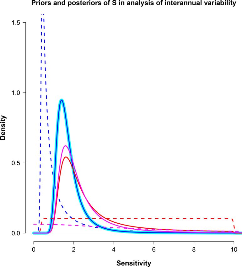
348                                                                             J. D. Annan and J. C. Hargreaves: Implicit priors

give some alternate analyses based on alternative, explicitly       tervals so generated would include the true value xT . How-
stated, priors. We argue that this latter approach is preferred,    ever, frequentist confidence intervals are not the same thing
as it both clarifies the role of the prior and allows researchers   as Bayesian credible intervals. The latter interpretation for an
to transparently test the sensitivity of their results to it. We    interval refers to a degree of belief that the particular interval
conclude with a general discussion about our results.               that has been generated on a specific occasion does in fact
                                                                    include the parameter. Climate scientists are far from unique
2     Principles and methods                                        in this misinterpretation, which appears to be widespread
                                                                    throughout the scientific community (Hoekstra et al., 2014).
2.1    Confidence intervals, Bayesian probability, and the          Because this misunderstanding is so deeply embedded in sci-
       “confusion of the inverse”                                   entific practice and discourse, we now discuss and explain it
                                                                    in some detail.
Let us assume we have a measuring process that produces an             We start by noting that probabilistic statements concerning
observational estimate xo of an unknown (but assumed con-           the true value xT demand the use of the Bayesian paradigm
stant) parameter which takes the value xT , with an observa-        wherein the language and mathematics of probability may be
tional error  that can be considered to take a specified error     applied to events that are not intrinsically random, but about
distribution, typically an unbiased Gaussian:                       which our knowledge is uncertain (Bernardo and Smith,
xo = xT + ,                                                 (1)    1994). The parameter xT itself does not have a probability
                                                                    distribution here; it was assumed to take a fixed value. There-
where  ∼ N(0, σ ). For simplicity, we assume here that σ is        fore, to even talk of the PDF of xT in this manner is to commit
known. This “measurement model” is fundamental to anal-             a category error. It is the researcher’s beliefs concerning xT
ysis of observations in many scientific domains. For exam-          that are uncertain, and this uncertainty is represented as their
ple, in climate science, analyses of observed global temper-        PDF for xT .
ature anomalies are commonly generated and presented in                Bayes’ theorem is a simple consequence of the axioms of
this form. We emphasise that the error term in this equation        probability: the joint density p(xo , xT ) of two variables xo
need not be defined solely in terms of a simple instrumen-          and xT can be decomposed in two different ways via
tal or sampling error but may include any and all sources of
discrepancy between the numerical value generated from an           p (xo , xT ) = p (xT |xo ) p (xo ) = p (xo |xT ) p (xT )
observational analysis and the measurand that the researcher        and thus
is interested in. Some examples will be discussed later when
we present applications of our methodology. All that we re-         p (xT |xo ) = p (xo |xT ) p (xT ) /p (xo ) .                  (2)
quire in order to use this equation is to assume that the uncer-
tainty inherent in the generation of the observational estimate     p(xT |xo ) is our posterior density for the true value xT given
is independent of the true value which is being estimated and       the observational evidence xo . p(xT ) is the prior distribution
that we have a statistical model for it (such as Gaussian).         for xT , which describes the researcher’s belief excluding the
   Following on from this measurement model, there is a sim-        observational evidence. p(xo |xT ) is commonly termed the
ple syllogism (i.e. a logical argument) that seems common           “likelihood” and is determined by the measurement model:
in many areas of scientific research, which runs as follows:        for example, in the case of an unbiased Gaussian obser-
since we know a priori that p(−2σ <  < 2σ ) ' 95 %, we             vational error, such as in Eq. (1), the functional form of
can also write a posteriori that p(xo − 2σ < xT < xo + 2σ ) '       p(xo |xT ) is given by
95 % once xo is known. For example, if σ = 0.25 is given and                        1    −(xo −xT )   2

we observe the value xo = 74.60, then the researcher may            p (xo |xT ) = √     e 2σ 2 .
assert that there is a ∼ 95 % probability that xT lies in the                      2π σ
interval (74.10, 75.10) or simply present a full probability        When the terms for xo and σ are replaced in this function
density: the probability distribution function (PDF) of xT is       by their known numerical values, this function looks like it
N(xo , σ ) = N(74.60, 0.25).                                        could be a probability distribution for p(xT |xo ), but as Bayes’
   This syllogism is intuitively appealing but incorrect. It        theorem (Eq. 2) makes clear, it is not in general the posterior
appears to arise from the misinterpretation of frequentist          PDF, instead being merely one term in its calculation. This
confidence intervals as being Bayesian credible intervals.          is the critical point which underpins the analyses presented
We should note that calculating and presenting the interval         in this paper: the distribution of the observation defined by
xo ± 2σ as a frequentist 95 % confidence interval would be          measurement models such as Eq. (1) directly defines the like-
a valid procedure. That is to say, if we were to repeatedly         lihood p(xo |xT ) and not the posterior PDF p(xT |xo ).
take a new observation xo according to Eq. (1), with each ob-          The error in the syllogism is to interpret p(xo |xT )
servation having an independent observational error of stan-        as p(xT |xo ): this is a common fallacy known as the confu-
dard deviation 0.25, and generate the corresponding inter-          sion of the inverse, which is closely related to the “prosecu-
val (xo − 0.5, xo + 0.5) then approximately 95 % of the in-         tor’s fallacy”, the latter term generally being used in discrete

Earth Syst. Dynam., 11, 347–356, 2020                                                    www.earth-syst-dynam.net/11/347/2020/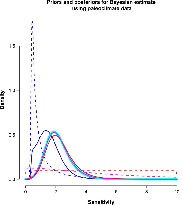
J. D. Annan and J. C. Hargreaves: Implicit priors                                                                               349
                                                                                                      √
probability in which the phenomenon is more widely known            a height drop h is given by t = 2h/a, where a = 9.8 m s−2
and well studied. The fallacy is perhaps easiest to illustrate      is the acceleration due to gravity. Due to the substantial ob-
with discrete cases which compare P (A|B) to P (B|A) for            servational uncertainty, the likelihood of the drop time is vir-
a pair of events A and B. For example, the probability of           tually flat across the support of the prior, varying by less
a person suffering from a rare disease (event A), given that        than 1 % across the range of 1.60 to 1.90 m. The posterior
they tested positive for it (event B), is in general different      estimate obtained through Bayes’ theorem is easily calcu-
from (and often rather lower than) the probability that some-       lated by direct numerical integration and still approximates
one produces a positive test result given that they are suf-        to N(1.75, 0.07) to two decimal places. The correct interpre-
fering from the disease. It has been known for some time            tation of the experiment is not, therefore, that the measure-
that medical doctors routinely commit this transposition er-        ment shows there is a substantial probability of the researcher
ror (Gigerenzer and Hoffrage, 1995). Additional examples            breaking a height record, but rather that the measurement is
and a further discussion of this type of fallacious reasoning       so imprecise that it does not add any significant information
in relation to interval estimation can be found in Morey et al.     on top of what was already known.
(2016).                                                                While it is formally invalid, we must acknowledge that this
   We now present a simple example in which the syllogism           syllogism does actually work rather well in many cases. In
leads to poor results in a physically based scenario with con-      particular, if the likelihood p(xo |xT ) is non-negligible over a
tinuous data. We take as given that the timing error of a           sufficiently small neighbourhood of xo such that a prior can
handheld stopwatch is ±0.25 s at 1 standard deviation (Het-         reasonably be used which is close to uniform in this region
zler et al., 2008). That is to say, the measured time to is re-     of xo , then the true posterior calculated by a Bayesian analy-
lated to the true time, tT , via to = tT +  with  ∼ N (0, 0.25)   sis will be close to that asserted by the syllogism. For exam-
(see Eq. 1). Let us consider an experiment in which an adult        ple, if the Gaussian prior xT ∼ N (100, 20) were to be used in
male colleague holds a dense object (say, a stone) at head          the original example, then when this is updated by the like-
height while standing and drops it while the experimenter           lihood corresponding to the observation xo = 74.6 with un-
times how long it takes for the stone to reach the ground.          certainty σ = 0.25, the correct posterior p(xT |xo ) is actually
   An observed time of to = 0.60 s could lead someone to            given by N(74.6, 0.25) to several significant digits. In the
say via the confusion of the inverse fallacy that the true time     limiting case in which an unbounded uniform prior is used
taken is represented by the Gaussian PDF tT ∼ N(0.6, 0.25)          for xT , the syllogism is precisely correct.
(albeit with an assumed truncation at zero which we ignore             Thus, in practice the syllogism can often be interpreted as
for convenience). One implication of this PDF is that there is      a Bayesian analysis in which a uniform prior has been im-
a 16 % chance that the true time is less than 0.35 s and also       plicitly used, and in cases in which this is reasonable it will
a 16 % chance that it is more than 0.85 s. Ignoring the neg-        generate perfectly acceptable results. Statements to this ef-
ligible air resistance and using the simple equation of mo-         fect have occasionally appeared in some papers wherein a
tion under gravity h = 21 at 2 , one would have no choice but       non-Bayesian analysis has been presented as directly giving
to conclude from these values that the experimenter’s col-          rise to a posterior PDF. It may therefore seem that the terms
league has a 16 % chance of being less than 60 cm tall and          “fallacy” and “confusion” are somewhat melodramatic: this
also a 16 % chance of being greater than 4.5 m tall. For a typ-     convenient shortcut is often harmless enough. However, this
ical adult male, neither of these cases seems reasonable. We        cannot be simply asserted without proof: there are many ex-
have obtained a measurement which is entirely unremark-             amples of procedures for generating frequentist confidence
able, with the observed time corresponding to a fall of around      intervals in which the results cannot plausibly be interpreted
1.75 m. And yet the commonplace interpretation of an impre-         as Bayesian credible intervals (Morey et al., 2016). In addi-
cise measurement as directly giving rise to a probability dis-      tion to concerns over the prior, it is also essential when tak-
tribution for the measurand has led to palpably ridiculous re-      ing this shortcut that the observational uncertainty σ is taken
sults. While in many cases the results will not be so silly, this   to be a constant which does not vary with the parameter of
simple example does demonstrate that the methodology can-           interest xT . This may be the case when we consider uncer-
not be sound. The more pernicious cases are those in which          tainties arising solely from an observational instrument but
the interpretation is not so obviously silly and thus may be        is less clear when σ includes a contribution from the system
confidently presented, even though the methodology is still         under study. For example, if the uncertainty in an observed
(as we have just shown) invalid.                                    estimate of the forced temperature response in an analysis
   In order to make sensible use of this observation, we can        of climate change includes a contribution due to the internal
instead perform a simple Bayesian updating procedure. The           variability of the climate system, then this internal variability
distribution N (0.6, 0.25) is actually correctly interpreted as     might be expected to vary with the parameters of the system.
the likelihood of the observed time p(to |tT ), which can be        In this case, an answer generated via the confusion of the in-
used to update a prior estimate. The distribution of adult male     verse cannot be rescued by the invocation of a uniform prior.
heights in the UK (in metres) is taken to be N(1.75, 0.07),         However, we do not explore this uncertainty in σ further in
and we use this as our prior. The drop time t predicted from        this paper.

www.earth-syst-dynam.net/11/347/2020/                                                   Earth Syst. Dynam., 11, 347–356, 2020
350 J. D. Annan and J. C. Hargreaves: Implicit priors
Some have attempted to retrospectively defend the use of CO2 ). In fact, both of these improper priors can exhibit a
this syllogism with the claim that the uniform prior is neces- pathology which causes problems with their use. In particu-
sarily the correct one to use, generally via the belief that this lar, if the likelihood is non-zero at λ = 0 (S = 0), then when
represents some sort of pure or maximal state of ignorance. the improper unbounded uniform prior on S (λ) is used, the
However, it is well established (and indeed is sometimes used posterior will also be improper and unbounded. In practi-
as a specific point of criticism) that there is no such thing as cal applications, this problem has generally been masked by
pure ignorance within the Bayesian framework. See Annan the use of an upper bound on the prior, but (while a lower
and Hargreaves (2011) for a further discussion of this in the bound of 0 may be defended on the basis of stability) the
context of climate science. Our objection to the widespread choice of the upper bound is hard to justify. The upper bound
application of this procedure is perhaps best summed up by which appears to have been most commonly used for sensi-
Morey et al. (2016), who state the following: “Using con- tivity is 10 ◦ C, and we will adopt this choice here. We use
fidence intervals as if they were credible intervals is an at- a range of 0.37–10 for the uniform priors in both λ and S,
tempt to smuggle Bayesian meaning into frequentist statis- which ensures that their ranges are numerically identical (al-
tics, without proper consideration of a prior.” There is also a though their units are of course different). As a third alterna-
strand of Bayesianism which asserts more broadly that in any tive prior for S, we will also use the positive half of a Cauchy
given experimental context there is a single preferred prior, prior, with location 0 and scale parameter 5, i.e. p(S) =
2
typically one which maximises the influence of the likelihood 5π(1+(S/5)2 )
, S > 0. An attractive feature of the Cauchy prior
in some well-defined manner. The Jeffreys prior is one com- is that it has a long tail which only decreases quadratically
mon approach within this “objective Bayesian” framework. (hence, it does not rule out high vales a priori); moreover,
However, it has the disadvantage that it assigns zero proba- its inverse is also Cauchy, so both S and λ have broad sup-
bility to events that the observations are uninformative about. port. The scale factor is the 50th percentile of the distribution;
This “see no evil” approach does have mathematical benefits hence, the half-Cauchy prior for S has a 50 % probability of
but it is hard to accept as a robust method if the results of the exceeding 5 ◦ C. The scale factor of the corresponding im-
analysis are intended to be of practical use. In the real world, plied prior in λ is given by 3.7/5 = 0.74 W m−2 K−1 .
our inability to (currently) observe something cannot ratio-
nally be considered sufficient reason to rule it out. We do not
3 Applications
consider objective Bayesian approaches further.
It is a fundamental assumption of this paper that in the We now consider three areas in which observational con-
cases presented below, in which researchers have presented straints have been used to estimate the equilibrium cli-
observational estimates of temperature change 1To in the mate sensitivity. Firstly, we consider paleoclimatic evidence,
form 1To = µ ± σ or in some equivalent manner, they are which relates to intervals during which the climate was rea-
(perhaps implicitly) using a measurement model of the form sonably stable over a long period of time and significantly
given in Eq. (1) with µ representing the observational value different to the pre-industrial state. We then consider analy-
obtained and σ representing the expected magnitude of ob- ses of observations of the warming trend over the 20th cen-
servational uncertainty (assumed Gaussian throughout this tury (strictly, extending into the 21st and 19th century). Fi-
paper, as is common in the literature). On this basis, the tem- nally, we consider analyses of interannual variability.
perature observation gives rise to a likelihood as described
above and does not directly generate a probability distribu-
3.1 Paleoclimate
tion for 1TT . We note, however, that authors have not always
been entirely clear about the statistical framework of their 3.1.1 Observationally derived PDFs
work and it is not always possible to discern their intentions
precisely. Thus, while we confidently believe our interpreta- A common paradigm for estimating the equilibrium climate
tion to be natural and appropriate in many cases, we do not sensitivity S using paleoclimatic data is to consider an in-
claim it to be universally applicable. terval in which the climate was reasonably stable and signifi-
cantly different to the present and analyse proxy data, such as
pollen grains and isotopic ratios in sediment cores, in order
2.2 Priors for the climate sensitivity to generate estimates of the forced global mean temperature
Most probabilistic estimates of the equilibrium climate sensi- anomaly 1T caused by the forcing anomaly 1F relative to
tivity which have explicitly presented a Bayesian framework the current (pre-industrial) climate. S can then be estimated
have used a prior which is uniform in sensitivity S. There via the equation
does not appear to be any principled basis for this choice, S = F2× × 1T /1F, (3)
which has been argued on the basis that it represented “ig-
norance”. One could just as easily (and erroneously) argue where F2× is the forcing due to a doubling of the atmospheric
that a prior which is uniform in feedback λ = F2× /S was ig- CO2 concentration. Examples of this approach include An-
norant (here F2× is the forcing arising from a doubling of nan and Hargreaves (2006) and Rohling et al. (2012).
Earth Syst. Dynam., 11, 347–356, 2020 www.earth-syst-dynam.net/11/347/2020/J. D. Annan and J. C. Hargreaves: Implicit priors 351
The interval which has been examined in the most detail
in this manner is probably the Last Glacial Maximum at 19–
23 ka (Mix et al., 2001) when the climate was reasonably
stable (at least in the sense of gross evaluations such as global
mean surface air temperature on millennial timescales) and
substantially different to the present day such that the signal-
to-noise ratio in estimates of forcing and temperature change
is reasonably high.
The method adopted by Annan and Hargreaves (2006) and
we believe many others (although this is not always doc-
umented explicitly), which we term sampling the observa-
tional PDFs, was to generate an ensemble of values of S by
repeatedly drawing pairs of samples from PDFs, which are
deemed to represent estimates of the forcing and tempera-
ture anomalies, and calculating for each pair the correspond-
ing value of S using Eq. (3). The ensemble of values for S
so generated is then considered to be a representative sample
from a probabilistic estimate of the truth.
Using values based broadly on those used in Annan and
Hargreaves (2006, 2013), Köhler et al. (2010), and Rohling
et al. (2012), we use observational estimates of 5 ± 1.5 ◦ C
for 1T and 9 ± 2 W m−2 for 1F (with the uncertainties here
assumed to represent 1 standard deviation of a Gaussian),
along with a fixed value for F2× of 3.7 W m−2 . In the illus- Figure 1. Prior and posterior estimates for the climate sensitivity
trative calculations presented here we ignore any issues relat- arising from paleoclimatic evidence. Dashed lines show priors, and
ing to the non-constancy of the sensitivity S and how it might solid lines are posterior densities. The thick cyan line shows the
vary in relation to the background climate state and nature of posterior estimate arising from the method of sampling observa-
the forcing, although we have slightly inflated the uncertain- tional PDFs, with the corresponding prior shown in Fig. 2. Blue
lines represent results using a uniform prior in λ; red is uniform
ties of the observational constraints in order to make some
in S, and magenta is half-Cauchy (scale: 5) in S (and therefore also
attempt to compensate for this. Thus, the numerical values
half-Cauchy in λ; scale: 3.7/5).
generated here are not intended to be definitive but are still
adequate to illustrate the different approaches.
As mentioned in Sect. 2.1, we assume that published es- researchers might prefer to make different choices, in partic-
timates for 1T can be understood as representing likeli- ular if they could clearly identify a likelihood arising from
hoods p(1To |1TT ) – that is to say, the observational anal- observational data.
ysis provides an uncertain estimate of the true value of the When applied to the numerical estimates provided above,
form given by Eq. (1) with an a priori unbiased error of the PDF sampling method of Annan and Hargreaves (2006)
the specified value. The analysis of Annan and Hargreaves generates an ensemble for S with a median estimate of 2.1 ◦ C
(2013) certainly follows this paradigm, with the estimate of and a 5 %–95% range of 1.0 to 3.8 ◦ C. Figure 1 presents this
the uncertainty being informed by a series of numerical ex- result as the cyan line, together with additional results which
periments in which the estimation procedure was tested on will be described below.
artificial datasets in order to calibrate its performance. For
the forcing estimate, things are not so clear. We do not have 3.1.2 Bayesian interpretation and alternative priors
direct proxy-based evidence for the forcing, which is typi-
cally estimated based on a combination of modelling results Now we present alternative calculations which take a more
and some rather subjective judgements (Köhler et al., 2010; standard and explicitly Bayesian approach. We start by writ-
Rohling et al., 2012). Any uncertainty in the actual measure- ing the model in the form
ments involved, such as those of greenhouse gas concentra-
tions in bubbles in ice cores, makes a negligible contribu- 1T = S × 1F /3.7, (4)
tion to the overall uncertainty in total forcing. Therefore, we
or equivalently
do not have a clear measurement model of the form given
in Eq. (1) with which to define a likelihood for the forcing. 1T = 1F /λ, (5)
Thus, we take the stated distribution to directly represent a
prior estimate for the forcing anomaly. We do not claim that where λ = S/3.7 is the feedback parameter. This formula-
this is the only reasonable approach to take here, and other tion allows us to easily consider the forcing and feedback
www.earth-syst-dynam.net/11/347/2020/ Earth Syst. Dynam., 11, 347–356, 2020352 J. D. Annan and J. C. Hargreaves: Implicit priors
parameter to be uncertain inputs (for which we can explicitly
define prior distributions) to the model, which can then be
updated by the likelihood arising from the observed temper-
ature change.
Although the method of sampling observational PDFs de-
scribed in Sect. 3.1.1 was not presented in Bayesian terms,
we are now in a position to present a Bayesian interpreta-
tion of it. The distribution generated by sampling the PDFs
is distributed as independently Gaussian N(5, 1.5) in 1T and
Gaussian N (9, 2) in 1F . We aim to choose a prior such that
the Bayesian analysis will generate this as the posterior after
updating by the likelihood for 1T . This likelihood as de-
scribed above is taken to be the Gaussian N (5, 1.5). There-
fore, by rearrangement of Bayes’ theorem, the desired prior
must be uniform in 1T and independently Gaussian N(9, 2)
in 1F . For numerical reasons we must impose bounds on the
uniform prior for 1T , and we set this range to be 0–20 ◦ C.
Using Eq. (3), we can re-parameterise this joint prior dis-
tribution over 1T and 1F into a distribution over S and 1F ,
and this is presented in Fig. 2. Note that this prior cannot
be represented as the product of independent distributions
over S and 1F , as high S here is correlated with low 1F and
vice versa. The prior in S when viewed as a marginal distri-
bution (i.e. after integrating over 1F ) appears uniform over
a significant range (roughly between S = 0.6 and S = 5), but
Figure 2. Implicit prior used in the paleoclimate estimate. The con-
within this range it is associated with somewhat high val-
tour plot shows the joint prior in S and 1F with marginal densi-
ues for 1F , with the latter taking a mean value of about
ties shown at the top and right, respectively. Vertical and horizontal
9.5 W m−2 over this region. The details of the shape of this dashed lines are drawn at S = 0.6, 5, and 1F = 9.
joint prior depend on the bounds placed on the uniform prior
for 1T , but this does not affect the posterior so long as the
prior is broad enough to cover the neighbourhood of the estimation, which is perhaps not surprising given the large
observation. We think it is unlikely that researchers would uncertainties in the observational constraints used here. The
choose a joint prior of this form deliberately and confirm median posterior value for S obtained from the half-Cauchy
that this certainly was not the case in Annan and Hargreaves prior is 2.1 ◦ C with a 5 %–95% range of 1.0–3.8 ◦ C, which
(2006). In future analyses it would seem more appropriate to coincidentally aligns very closely with the result obtained by
clearly state the priors which are used and test the sensitivity the naive method of sampling observational PDFs (which is
of the results to this choice. plotted as a thick line in Fig. 1 in order to make it more vis-
In order to perform a more conventional Bayesian updat- ible). We conclude in this case that the method of sampling
ing procedure using Eq. (5), we must first select priors on the PDFs has generated a result which is reasonable, but alter-
model inputs. Since the sensitivity is a property of the cli- native choices of the prior could give noticeably different re-
mate system, whereas the forcing is specific to the interval sults.
we are considering, we define their priors independently. For
the forcing 1F , we retain the N(9, 2) prior, having no plausi-
ble basis for trying anything different. For sensitivity, we test 3.2 Estimates based on historical warming
the three priors described in Sect. 2.2. The two uniform priors 3.2.1 Observationally derived PDFs
generate rather different results. Using a prior which is uni-
form in S, the posterior has a mean value for S of 2.2 ◦ C and Perhaps the most common approach to estimating S has been
a 5 %–95% range of 1.0–4.2 ◦ C. When we change to uniform to use the instrumental record (Tol and De Vos, 1998; Gre-
in λ the median decreases to 1.5 ◦ C with a 5 %–95% range of gory et al., 2002; Olson et al., 2012; Aldrin et al., 2012).
0.5–3.0 ◦ C. While these results, which are shown in Fig. 1, While a wide range of climate models have been utilised
overlap substantially, broadening the upper bounds on the for this purpose, a simple energy balance similar to that of
priors would result in the first result increasing without limit Sect. 3.1 can be used so long as the radiative imbalance is
and the second decreasing towards zero such that they would accounted for. We follow the recent analysis of Mauritsen
fully separate. We therefore see that extreme choices for the and Pincus (2017) but simplify their calculation by ignor-
prior on S (or λ) can have a significant influence on Bayesian ing uncertainty in F2× , instead adopting their mean value of
Earth Syst. Dynam., 11, 347–356, 2020 www.earth-syst-dynam.net/11/347/2020/J. D. Annan and J. C. Hargreaves: Implicit priors 353
3.71 W m−2 (using all their uncertain numerical values oth-
erwise). This simplification has very little influence on the
results. Mauritsen and Pincus (2017) present the basic en-
ergy balance in the form
S = F2× 1T /(1F − 1Q), (6)
where 1Q represents the net planetary radiative imbalance
and the other terms are as before. We emphasise that 1T here
specifically denotes the forced temperature change. This
equation is applied between two widely separated decadal-
scale intervals within the historical record such that the
signal-to-noise ratio in the temperature change (and hence
precision in the resulting estimate of S) is as large as pos-
sible, though it remains a significant source of uncertainty
(Dessler et al., 2018). Similar to Sect. 3.1.1, the method used
by Mauritsen and Pincus (2017) is one of sampling obser-
vationally derived PDFs for all uncertain quantities on the
right-hand side of Eq. (6), thereby generating an ensemble of
values for S which was interpreted as a probability distribu-
tion.
3.2.2 Bayesian interpretation and alternative priors
As in Sect. 3.1.2, we reorganise Eq. (6) in order to give 1T Figure 3. Implicit prior used in the 20th century estimate.
as the prognostic variable, assigning priors to the terms on
the right-hand side. We thus obtain
minor simplification to their calculation. The posterior me-
1T = (1F − 1Q) × S/F2× = (1F − 1Q)/λ. (7) dian calculated here is 1.8 ◦ C with a 5 %–95% range of 1.1–
4.5 ◦ C. As in Sect. 3.1, we make no attempt to decompose
We adopt the distributions used by Mauritsen and Pincus
the forcing estimate used here into a prior and likelihood,
(2017) for 1F and 1Q as priors for these variables but inter-
especially as some of the largest uncertainties (e.g. that aris-
pret their estimate for the temperature change 1To as a like-
ing from aerosol forcing) are based on modelling calculations
lihood p(1To |1T ) ∼ N(0.77, 0.08) arising from the mea-
and expert judgements that cannot be transparently traced to
surement model of Eq. (1). This arises immediately from the
uncertainties in observational data.
paradigm of the observed total temperature response consist-
Alternative priors and their resulting posteriors after
ing of the forced response summed together with a contribu-
Bayesian updating using Eq. (7) are shown in Fig. 4. As
tion from internal variability which can be assumed indepen-
before, we test the three priors presented in Sect. 2.2. The
dent of the forced response itself. In this case, the analysis
posterior median values (and 5 %–95% range) for S aris-
of observed temperatures generated the (deterministic) value
ing from these are 2.1 ◦ C (1.2–6.3 ◦ C) for uniform S, 1.5 ◦ C
1To = 0.77 ◦ C, with the uncertainty estimate being sepa-
(1.0–3.1 ◦ C) for uniform λ, and 2.0 ◦ C (1.1–5.0 ◦ C) for the
rately derived as an estimate for the likely contribution of
half-Cauchy prior. Thus, again the half-Cauchy prior pro-
internal variability to a temperature change over such a time
duces a result which is intermediate between the other ex-
interval (Lewis and Curry, 2014). True measurement errors
plicit choices, though this time it has a somewhat longer
in the calculation of 1To are sufficiently small relative to this
tail than the PDF sampling method. The differences between
internal variability that they can be safely ignored.
these results, especially for the upper 95 % limit, are sub-
Given the similarities between Eqs. (3) and (6), and also in
stantial and could significantly alter their interpretation and
the method used, it is no surprise to find that the implicit prior
impact.
used here before updating with the temperature likelihood is
qualitatively similar to that found in Sect. 3.1. This is shown
in Fig. 3. Again, the marginal prior over S appears uniform 3.3 Estimates based on interannual variability
over a reasonable range (the details depend on the limits of 3.3.1 Observationally derived PDFs
the uniform prior over 1T ), but nevertheless it is actually
correlated with the net forcing. Figure 4 shows the posterior Finally, we consider a method which has been used to es-
result arising from this prior, which matches the published timate the climate sensitivity via interannual variation in
result of Mauritsen and Pincus (2017) closely despite our the radiation balance and temperature (Forster and Gregory,
www.earth-syst-dynam.net/11/347/2020/ Earth Syst. Dynam., 11, 347–356, 2020354 J. D. Annan and J. C. Hargreaves: Implicit priors
Figure 4. Priors and posteriors in explicit Bayesian estimates us- Figure 5. Priors and posteriors over S in a process-based feedback
ing 20th century data. Dashed lines show priors, and solid lines are analysis. Dashed lines indicate priors, and solid lines are posteriors.
posterior densities. The thick cyan line shows the posterior estimate The thick cyan line shows the posterior estimate arising from the
arising from the method of sampling observational PDFs, with its method of sampling observational PDFs, which coincides precisely
implicit prior shown in Fig. 3. Blue lines represent results using a with the blue line that corresponds to the uniform prior in λ. Red
uniform prior in λ; red is uniform in S, and magenta is half-Cauchy lines show results using a uniform prior in S, and magenta is half-
(scale: 5) in S (and therefore also half-Cauchy in λ; scale: 3.7/5). Cauchy (scale: 5) in S.
Therefore, a likelihood for λ can be directly interpreted as an
equivalent likelihood for S.
2006; Dessler and Forster, 2018). The basic premise of these
analyses is that the feedback parameter can be estimated as 3.3.2 Bayesian interpretation and alternative priors
the slope of the regression line of the net radiation imbalance
(based primarily on satellite observations) against tempera- As noted by Forster and Gregory (2006), presenting what ac-
ture anomalies, with data typically averaged on an annual tually amounts to an observational likelihood for λ as a pos-
timescale (though seasonal data may also be used). There terior PDF is equivalent to assuming a uniform prior in λ (see
are questions as to whether this short-term variability pro- also Annan and Hargreaves, 2011). Therefore, the Bayesian
vides an accurate estimate of long-term changes, but this is interpretation is already clear in this instance.
beyond the scope of this paper (Dessler and Forster, 2018). In Fig. 5 we present the results of calculations using our
The regression slope and its uncertainty naturally translate three alternative priors (although one of them coincides with
into a Gaussian likelihood for the true feedback component the method of sampling PDFs). The original result of Forster
and have been commonly interpreted as a probability distri- and Gregory (2006) (after transforming to S space) is rep-
bution for λ. While this again appears on the face of it to resented by the blue lines, with red showing the result ob-
commit the fallacy of confusion of the inverse, the implicit tained for a uniform prior in S and magenta being a Cauchy
assumption of a uniform prior on λ that underpins this inter- prior. We note that, for the uniform S case, if the upper bound
pretation has been clearly acknowledged by authors working on the prior was raised, the posterior would also increase
in this area (e.g. see comments in Forster and Gregory, 2006; without limit due to the pathological behaviour discussed
Forster, 2016). In this section we will use the observational in Sect. 3.1.2 and also by Annan and Hargreaves (2011).
estimate of Forster and Gregory (2006), which is given by For the priors shown (with the uniform priors defined as
λo = 2.3±0.7 W m−2 K−1 . We note that when uncertainty in U [0.37, 10]) the 5 %–95% ranges of the posteriors are 1.1–
the forcing arising from a doubling of CO2 is ignored, there 3.2, 1.2–6.9, and 1.2–5.2 ◦ C for the uniform λ, uniform S,
is a trivial transformation between λ and S via S = F2× /λ. and Cauchy S priors, respectively. The uniform λ prior com-
Earth Syst. Dynam., 11, 347–356, 2020 www.earth-syst-dynam.net/11/347/2020/J. D. Annan and J. C. Hargreaves: Implicit priors 355
monly adopted by analyses of this type provides a strong ten- Diagnosis and Intercomparison (PCMDI), and the WCRP’s Work-
dency towards low values, and the contrast with uniform S, ing Group on Coupled Modelling (WGCM) for their roles in mak-
especially for the upper bound, is disconcerting. ing available the WCRP CMIP3 multi-model dataset. Support for
this dataset is provided by the Office of Science, US Department of
Energy.
4 Conclusions
We have shown how various calculations which have pre- Review statement. This paper was edited by Michel Crucifix and
sented probabilistic estimates of the equilibrium climate sen- reviewed by two anonymous referees.
sitivity S can be reinterpreted within a standard Bayesian
framework. Using this standard framework ensures a clear
distinction between the prior choices, which must be made References
for model parameters and inputs, and the likelihood obtained
from observations of the system, which is then used to update Aldrin, M., Holden, M., Guttorp, P., Skeie, R. B., Myhre, G., and
this prior in order to generate the posterior. Berntsen, T. K.: Bayesian estimation of climate sensitivity based
In many cases, the implied prior for S which (according on a simple climate model fitted to observations of hemispheric
to this interpretation) underlies the published results appears temperatures and global ocean heat content, Environmetrics, 23,
somewhat unnatural, having either a structural relationship 253–271, https://doi.org/10.1002/env.2140, 2012.
Annan, J. D. and Hargreaves, J. C.: Using multiple observationally-
with model inputs or a marginal distribution that may not be
based constraints to estimate climate sensitivity, Geophys. Res.
considered reasonable. We have presented alternative calcu-
Lett., 33, L06704, https://doi.org/10.1029/2005GL025259, 2006.
lations in which a range of simple priors are tested. In addi- Annan, J. D. and Hargreaves, J. C.: On the generation and inter-
tion to the commonly used uniform priors, we have shown pretation of probabilistic estimates of climate sensitivity, Cli-
that a Cauchy prior has some attractive features in that it ex- matic Change, 104, 423–436, https://doi.org/10.1007/s10584-
tends to high values (refuting any suspicion that the results 009-9715-y, 2011.
obtained were simply constrained by the prior), and its recip- Annan, J. D. and Hargreaves, J. C.: A new global reconstruction of
rocal is also Cauchy (so both S and λ may have long tails). temperature changes at the Last Glacial Maximum, Clim.e Past,
The half-Cauchy distribution used in this paper only requires 9, 367–376, https://doi.org/10.5194/cp-9-367-2013, 2013.
a single scale parameter which determines the width. How- Bernardo, J. and Smith, A.: Bayesian Theory, Wiley, Chichester,
ever, the choice of priors is always subjective, and we make UK, 1994.
Dessler, A. E. and Forster, P. M.: An estimate of equilibrium climate
no assertion that this choice should be universally adopted.
sensitivity from interannual variability, J. Geophys. Res.-Atmos.,
Indeed, there may be superior alternative choices that we 123, 8634–8645, https://doi.org/10.1029/2018JD028481, 2018.
have not considered. Dessler, A. E., Mauritsen, T., and Stevens, B.: The influence
Our calculations suggest that the PDF sampling method of internal variability on Earth’s energy balance framework
can generate acceptable results in some cases, agreeing fairly and implications for estimating climate sensitivity, Atmos.
well with a fully Bayesian approach using reasonable priors. Chem. Phys., 18, 5147–5155, https://doi.org/10.5194/acp-18-
However, this is not always the case. We recommend that 5147-2018, 2018.
researchers present their analysis in an explicitly Bayesian Forster, P. M.: Inference of climate sensitivity from analysis of
manner as we have done here, as this allows the influence of Earth’s energy budget, Annu. Rev. Earth Planet. Sci., 44, 85–106,
the prior and other uncertain inputs to be transparently tested. 2016.
Forster, P. M. and Gregory, J. M.: The Climate Sensitivity and Its
Components Diagnosed from Earth Radiation Budget Data, J.
Climate, 19, 39–52, https://doi.org/10.1175/JCLI3611.1, 2006.
Code availability. All codes used in this paper can be found in the
Gigerenzer, G. and Hoffrage, U.: How to improve Bayesian reason-
Supplement.
ing without instruction: frequency formats, Psycholog. Rev., 102,
684–704, 1995.
Gregory, J. M., Stouffer, R. J., Raper, S. C. B., Stott, P. A., and
Supplement. The supplement related to this article is available Rayner, N. A.: An observationally based estimate of the climate
online at: https://doi.org/10.5194/esd-11-347-2020-supplement. sensitivity, J. Climate, 15, 3117–3121, 2002.
Hetzler, R. K., Stickley, C. D., Lundquist, K. M., and Kimura, I. F.:
Reliability and accuracy of handheld stopwatches compared with
Author contributions. Both authors contributed to the research electronic timing in measuring sprint performance, J. Streng.
and writing. Condit. Res., 22, 1969–1976, 2008.
Hoekstra, R., Morey, R. D., Rouder, J. N., and Wagenmakers, E.-
J.: Robust misinterpretation of confidence intervals, Psychonom.
Acknowledgements. We are grateful to Andrew Dessler and two Bull. Rev., 21, 1157–1164, 2014.
anonymous referees for helpful comments on the paper. We ac- Köhler, P., Bintanja, R., Fischer, H., Joos, F., Knutti, R., Lohmann,
knowledge the modelling groups, the Program for Climate Model G., and Masson-Delmotte, V.: What caused Earth’s temperature
www.earth-syst-dynam.net/11/347/2020/ Earth Syst. Dynam., 11, 347–356, 2020356 J. D. Annan and J. C. Hargreaves: Implicit priors variations during the last 800,000 years? Data-based evidence on Rohling, E., Sluijs, A., Dijkstra, H., Köhler, P., van de Wal, R., radiative forcing and constraints on climate sensitivity, Quater- von der Heydt, A., Beerling, D., Berger, A., Bijl, P., Crucifix, nary Sci. Rev., 29, 129–145, 2010. M., DeConto, R., Drijfhout, S. S., Fedorov, A., Foster, G. L., Lewis, N. and Curry, J. A.: The implications for climate sensitivity Ganopolski, A., Hansen, J., Hönisch, B., Hooghiemstra, H., Hu- of AR5 forcing and heat uptake estimates, Clim. Dynam., 45, ber, M., Huybers, P., Knutti, R., Lea, D. W., Lourens, L. J., Lunt, 1009–1023, https://doi.org/10.1007/s00382-014-2342-y, 2014. D., Masson-Delmotte, V., Medina-Elizalde, M., Otto-Bliesner, Mauritsen, T. and Pincus, R.: Committed warming inferred from B., Pagani, M., Pälike, H., Renssen, H., Royer, D. L., Siddall, observations, Nature Publishing Group, 7, 652–655, 2017. M., Valdes, P., Zachos, J. C., and Zeebe, R. E.: Making sense of Mix, A., Bard, E., and Schneider, R.: Environmental processes of palaeoclimate sensitivity, Nature, 491, 683–691, 2012. the ice age: land, oceans, glaciers (EPILOG), Quaternary Sci. Tol, R. S. and De Vos, A. F.: A Bayesian statistical analysis of the Rev., 20, 627–657, 2001. enhanced greenhouse effect, Climatic Change, 38, 87–112, 1998. Morey, R. D., Hoekstra, R., Rouder, J. N., Lee, M. D., and Wagen- makers, E.-J.: The fallacy of placing confidence in confidence intervals, Psychonom. Bull. Rev., 23, 103–123, 2016. Olson, R., Sriver, R., Goes, M., Urban, N. M., Matthews, H. D., Haran, M., and Keller, K.: A climate sensitivity esti- mate using Bayesian fusion of instrumental observations and an Earth System model, J. Geophys. Res., 117, D04103, https://doi.org/10.1029/2011JD016620, 2012. Earth Syst. Dynam., 11, 347–356, 2020 www.earth-syst-dynam.net/11/347/2020/
You can also read