Atlantic-Pacific seesaw and its role in outgassing CO2 during Heinrich events
←
→
Page content transcription
If your browser does not render page correctly, please read the page content below
PALEOCEANOGRAPHY, VOL. 29, 58–70, doi:10.1002/2013PA002542, 2014

Atlantic-Pacific seesaw and its role in outgassing CO2 during
Heinrich events
L. Menviel,1,2 M. H. England,1,2 K. J. Meissner,1,2 A. Mouchet,3,4 and J. Yu5
Received 31 July 2013; revised 4 December 2013; accepted 5 December 2013; published 30 January 2014.

[1] Paleoproxy records indicate that a marked weakening of the Atlantic Meridional
Overturning Circulation (AMOC) during Heinrich events was often accompanied by a
notable atmospheric CO2 increase. However, previous modeling studies display
conflicting atmospheric CO2 responses to an AMOC shutdown. Here we use model
simulations combined with paleoproxy records to show that depending on the deep and
bottom water transport in the Northern and Southern Pacific Ocean during an AMOC
weakening, the ocean can act either as a sink or a source of carbon. Results from
idealized meltwater experiments as well as from a transient experiment covering Heinrich
stadial 4 suggest that a shutdown of the AMOC during Heinrich stadials 4 (HS4) and 1
(HS1) led to an enhancement of Antarctic Bottom Water (AABW) and North Pacific
Deep Water (NPDW) transport. We show that enhanced deep and bottom water transport
in the Pacific Ocean ventilates deep Pacific carbon through the Southern Ocean, thus
contributing to a rise in atmospheric CO2 . This mechanism yields a good agreement
between paleoproxy records and modeling results, thus highlighting the possible
establishment of an Atlantic-Pacific seesaw during Heinrich stadials. Enhanced AABW
and NPDW transport could account for most of the observed atmospheric CO2 increase
during HS4 and for about 30% of the atmospheric CO2 increase during HS1.
Citation: Menviel, L., M. H. England, K. J. Meissner, A. Mouchet, and J. Yu (2014), Atlantic-Pacific seesaw and its role in
outgassing CO2 during Heinrich events, Paleoceanography, 29, 58–70, doi:10.1002/2013PA002542.

1. Introduction                                                                  climate change in the tropics [Deplazes et al., 2013], across
  [2] The last glacial period and the last deglaciation                          Asia [Tada et al., 1999; Wang et al., 2001], and through
were punctuated by millennial-scale events during which                          the bipolar seesaw effect, in Antarctica [Blunier and Brook,
the Atlantic Meridional Overturning Circulation (AMOC)                           2001]. However, not all Heinrich stadials display similar
weakened substantially [McManus et al., 2004]. These                             characteristics. Paleoproxy records suggest that Heinrich
events, called Heinrich events [Vidal et al., 1997], occurred                    stadial 4 (HS4, 40–38 ka B.P.) [Hemming, 2004], was asso-
most likely due to the addition of meltwater in the North                        ciated with a strong cooling over Greenland [Huber et al.,
Atlantic as a result of ice sheet instabilities [Heinrich, 1988].                2006] and the North Atlantic [Bard, 2002; Martrat et al.,
A weakening of the AMOC during Heinrich events had                               2007] as well as with a significant atmospheric CO2 increase
a strong impact on the climate around the North Atlantic                         at the beginning of the cool phase [Bereiter et al., 2012; Ahn
region [Dansgaard et al., 1993; Bond, 1993] and, via oceanic                     et al., 2012]. Paleorecords display little coherency regard-
and atmospheric teleconnections, it also led to significant                       ing the amplitude and the timing of Heinrich stadial 3,
                                                                                 maybe because in contrast to other Heinrich events, it origi-
                                                                                 nated from the Fennoscandian ice sheet [Elliot et al., 1998;
     Additional supporting information may be found in the online version        Snoeckx et al., 1999; Grousset et al., 2000] . Heinrich sta-
of this article.
    1
       Climate Change Research Centre, University of New South Wales,            dial 2 also displays a muted climatic response without any
Sydney, New South Wales, Australia.                                              discernible change in atmospheric CO2 [Ahn and Brook,
     2
       ARC Centre of Excellence for Climate System Science, Sydney, New          2008]. Finally Heinrich stadial 1 (HS1), which occurred
South Wales, Australia.                                                          right at the beginning of the last deglaciation, is associ-
     3
       Laboratoire des Sciences du Climat et de l’Environnement (LSCE),
IPSL-CEA-CNRS-UVSQ, Gif-sur-Yvette, France.
                                                                                 ated with an atmospheric CO2 increase, but it is still unclear
     4
       Astrophysics, Geophysics and Oceanography Department, Université          how much of this increase is due to the abrupt circulation
de Liège, Liège, Belgium.                                                        changes and how much is due to other processes linked to
     5
       Research School of Earth Sciences, Australian National University,        the deglaciation. Oceanic 14 C [Skinner et al., 2010; Burke
Canberra, ACT, Australia.                                                        and Robinson, 2012] and atmospheric ı 13 C records [Schmitt
   Corresponding author: L. Menviel, Climate Change Research Centre,             et al., 2012] indicate that greater Southern Ocean ventila-
University of New South Wales, Sydney, NSW 2052, Australia.                      tion during HS1 could have led to the observed atmospheric
(l.menviel@unsw.edu.au)                                                          CO2 rise.
©2013. American Geophysical Union. All Rights Reserved.                            [3] Previous studies examined either the terrestrial car-
0883-8305/14/10.1002/2013PA002542                                                bon response [Scholze et al., 2003; Köhler et al., 2005],
                                                                            58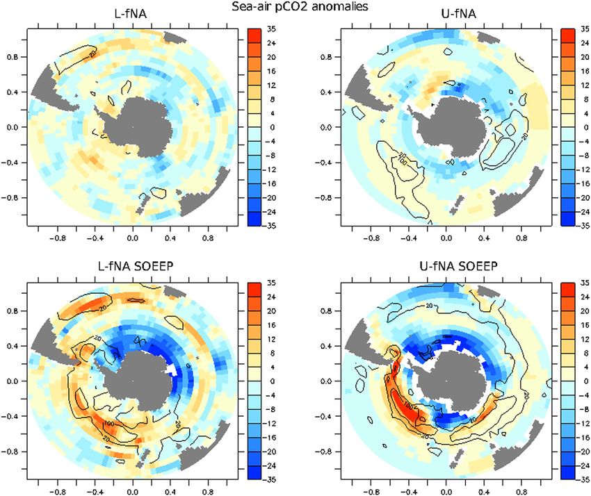
MENVIEL ET AL.: HEINRICH CO2

        Figure 1. Paleoproxy records of Heinrich event 1 compared to idealized meltwater experiments: (left)
        Paleoproxy records (where available) and (right) modeling results for experiments L-fNA (solid grey),
        L-fNASOEEP (solid red color), U-fNA (dashed grey), and U-fNASOEEP (dashed red color). Time series of
        (A) Freshwater flux (Sv) in the North Atlantic (grey) for all experiments and over the Southern Ocean
        and the EEP for L-fNASOEEP (red) and U-fNASOEEP (green). (b) Maximum overturning circulation during
        the deglaciation as recorded in marine sediment cores from the North Atlantic by McManus et al. [2004]
        (black) and Gherardi et al. [2005] (grey); (B) Maximum overturning circulation in the North Atlantic
        (Sv); (c) Compilation of ventilation ages (years) from Northwestern Pacific sediment cores [Okazaki et
        al., 2010], Benthic-Planktonic foraminifera ages (black circles) with 1 error bar, and smoothed spline
        interpolation of averaged BF-PF and projection ages (green); (C) North Pacific Deep Water transport
        anomaly (Sv); (d)  Nd from core RC11-83 in the South Atlantic [Piotrowski et al., 2005]; Note that the
        6 ka B.P. value is –9.3, thus indicating a greater proportion of AABW relative to NADW during HS1;
        (D) Antarctic Bottom Water transport anomaly in the Pacific Ocean (Sv). The AABW is calculated here
        as the maximum strength of the overturning in the abyssal cell at 35ı S and positive AABW indicates
        stronger AABW; (E) global export production anomalies (%) (f) opal flux (g/cm2 /kyr) in marine sedi-
        ment core TNO57-13PC from the South Atlantic [Anderson et al., 2009]; (F) opal production anomalies
        (%) for LOVECLIM and marine export production anomalies (%) for the UVic ESCM over the South
        Atlantic (50ı W–20ı E, 42ı S–60ı S); (G) Changes in PO4Pref /PO4Tot (%); (h) SSS anomalies in the South
        Pacific ocean as derived from planktic ı 18 O for core MD03-2611 [Calvo et al., 2007] (see section 2); (H)
        SSS anomaly averaged over the South Pacific Ocean (120ı E–200ı E, 35ı S–50ı S); (i) atmospheric CO2
        anomalies (ppmv) as recorded in the European Project for Ice Coring in Antarctica Dome C ice core,
        Antarctica [Parrenin et al., 2013]; (I) simulated atmospheric CO2 anomaly (ppmv). Please note that the
        ice core and simulated pCO2 are on different scales.

the marine carbon cycle response [Marchal et al., 1999;          2008; Bozbiyik et al., 2011; Bouttes et al., 2012; Huiskamp
Chikamoto et al., 2012], or the combined marine and ter-         and Meissner, 2012; Matsumoto and Yokoyama, 2013] to
restrial carbon response [Obata, 2007; Schmittner et al.,        an AMOC shutdown. While some modeling studies con-
2007; Menviel et al., 2008a; Schmittner and Galbraith,           cluded that the oceanic carbon content increased as a result
                                                            59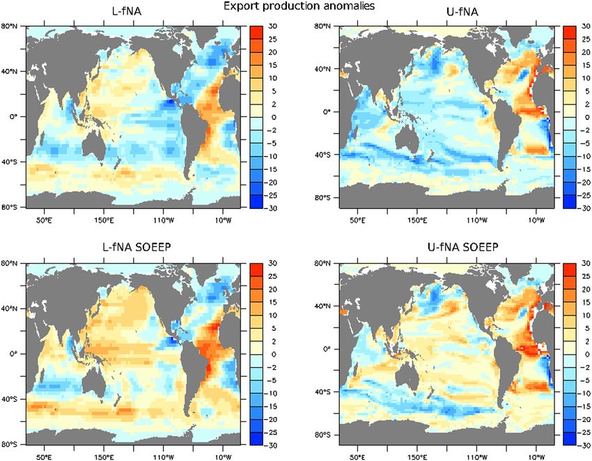
MENVIEL ET AL.: HEINRICH CO2

         Figure 2. Decomposition of CO2 changes for idealized meltwater experiments: Time series of (a) sim-
         ulated atmospheric CO2 anomaly (ppmv); (b) changes in atmospheric CO2 (ppmv) as calculated from the
         different contributions of SSS, SST, ALK, and DIC (see section 2); (c) global SSS (dashed, g/kg)
         and SST (solid, ı C) anomalies; (d) changes in atmospheric CO2 (ppmv) as calculated from SSS and
         SST; (e) changes in atmospheric CO2 (ppmv) resulting from global surface DIC (solid) and ALK
         (dashed); (f) changes in atmospheric CO2 (ppmv) resulting from the combined contribution of DIC and
         ALK for standard meltwater experiments performed with LOVECLIM (L-fNA, blue) and the UVic
         ESCM (U-fNA, black) as well as meltwater experiments with a negative freshwater flux in the Southern
         Ocean and EEP for LOVECLIM (L-fNASOEEP , red) and the UVic ESCM (U-fNASOEEP , green).

of an AMOC shutdown [Obata, 2007; Menviel et al., 2008a;              [4] Here we show that knowledge of changes not only
Bozbiyik et al., 2011; Chikamoto et al., 2012], others sug-         in North Atlantic Deep Water (NADW) but also in North
gested the opposite [Marchal et al., 1999; Schmittner et            Pacific Deep Water (NPDW) and Antarctic Bottom Water
al., 2007; Schmittner and Galbraith, 2008; Bouttes et al.,          (AABW) transport is required to fully understand the
2012; Matsumoto and Yokoyama, 2013]. Most of the studies            responses of the global climate and oceanic carbon cycle
[Marchal et al., 1999; Bouttes et al., 2012; Matsumoto and          during Heinrich events. We further suggest that a strength-
Yokoyama, 2013] which concluded that the oceanic carbon             ening of AABW and NPDW formation during HS1 and HS4
content decreased as a result of an AMOC shutdown, applied          caused a carbon release from the deep Pacific Ocean, thus
global salt compensation in their experimental design. Sim-         leading to an atmospheric CO2 increase.
ulating a shutdown of the AMOC due to an ice sheet
collapse presents some technical difficulties as the volume
of the ocean remains constant in most climate models. In            2. Methods
addition, freshwater pathways in the North Atlantic are
affected by model resolution [Condron and Winsor, 2011;             2.1. Model and Experimental Design
Spence et al., 2013]. It is thus likely that due to a combi-          [5] In this study we perform experiments with two Earth
nation of experimental design, model resolution, and other          System Models of Intermediate Complexity: LOVECLIM
model biases, standard meltwater experiments might not              1.1 [Goosse et al., 2010] and the University of Victoria
capture the past variability of Pacific deep and bottom water        Earth System Climate Model (UVic ESCM) v2.9 [Weaver
masses accurately.                                                  et al., 2001]. The ocean component of LOVECLIM (CLIO)
                                                               60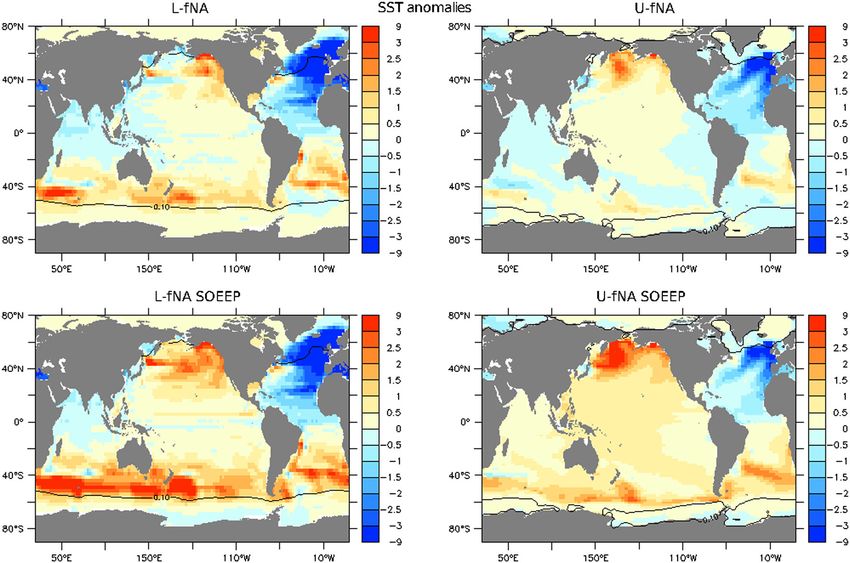
MENVIEL ET AL.: HEINRICH CO2
Table 1. Main Results of Idealized Experiments. Changes in Atmospheric CO2 and Carbon
Content (GtC) in the Atlantic, Pacific, Indian, and Arctic Basins as Well as in the Southern
Ocean at Model Years 1990–2000 Compared to the LGM Control Runa
pCO2 C Atl. C Pac. C Ind. C SO C Arctic
Exp. (ppmv) (GtC) (GtC) (GtC) (GtC) (GtC)
LOVECLIM
L-fNA –4.4 366 (216) –397 (–66) –40 24 57
L-fNASOEEP 9.8 344 (172) –430 (–218) –29 31 50
UVic
U-fNA –3.5 280 (167) –344 (–147) –12 41 40
U-fNASOEEP 24 302 (124) –408 (–314) 11 –7 48
a
For the Atlantic and Pacific basins, the first number represents changes integrated over all depths and
the number in brackets represents changes integrated over the deep ocean only (2000 m).
consists of a free-surface primitive equation model with marine carbon cycle model [Schmittner et al., 2008], and a
a horizontal resolution of 3ı longitude, 3ı latitude, and sediment model [Meissner et al., 2012].
20 depth layers. The atmospheric component (ECBilt) is a [6] First, some idealized experiments are performed with
spectral T21, three-level model based on quasi geostrophic LOVECLIM and the UVic ESCM under constant Last
equations of motion. LOVECLIM also includes a dynamic- Glacial Maximum (LGM, 21 ka B.P.) boundary conditions.
thermodynamic sea ice model, a land surface scheme, a A presentation of the performances of LOVECLIM and the
dynamic global vegetation model (VECODE), and a marine UVic ESCM under LGM conditions can be found in pre-
carbon cycle model (LOCH) [Menviel, 2008; Mouchet, vious publications [Menviel et al., 2008a; Meissner et al.,
2011]. The UVic ESCM consists of an ocean general cir- 2003a]. As the sea level was lower during glacial times,
culation model (Modular Ocean Model, Version 2) with a the Bering Strait is closed in all the experiments. Our study
resolution of 3.6ı longitude and 1.8ı latitude and coupled focuses on the marine carbon cycle response to a shut-
to a vertically integrated two-dimensional energy-moisture down of the AMOC. To avoid the marine carbon cycle
balance model of the atmosphere including a parameter- responding to changes in terrestrial carbon, the terrestrial
ization of geostrophic wind stress anomalies, a dynamic- carbon reservoir is kept constant at its LGM value in all
thermodynamic sea ice model, a land surface scheme, a the experiments performed here. We run two experiments
dynamic global vegetation model [Meissner et al., 2003b], a in which the AMOC is shut down through the addition
Figure 3. Sea Surface Salinity anomalies: SSS (g/kg) anomalies with respect to the LGM control run
averaged for model years 1990–2000 for (top) standard meltwater experiments and (bottom) meltwater
experiments with a negative freshwater input in the Southern Ocean and the EEP for (left) LOVECLIM
and (right) the UVic ESCM.
61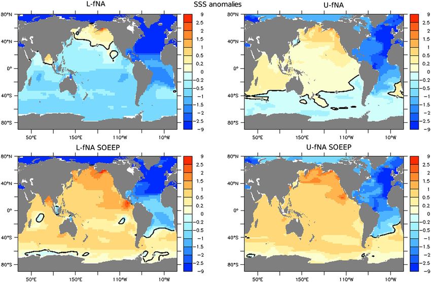
MENVIEL ET AL.: HEINRICH CO2

         Figure 4. Sea surface temperature anomalies: Same as Figure 3 but for SST (ı C) anomalies. Overlaid
         is the 0.1 m sea ice thickness contour for austral winter (JJA).

of 0.1 Sverdrup (Sv) (1 Sv = 106 m3 /s) freshwater in the               parameters [Berger, 1978], ice sheet topography and albedo
North Atlantic (55ı W–10ı W, 50ı N–65ı N) for 2000 years                [Abe-Ouchi et al., 2007], a closed Bering Strait, and an
(L-fNA and U-fNA, respectively, performed with LOVE-                    atmospheric CO2 content of 210 ppmv. Two transient exper-
CLIM and the UVic ESCM). Due to a combination of exper-                 iments (L-HS4 and L-HS4SOEEP ) are then integrated from
imental design, model resolution, and other model biases,               42 ka B.P. to 38.5 ka B.P. with all the transient forcing
we hypothesize that standard meltwater experiments might                described above and with prognostic atmospheric CO2 . In
generate anomalously low surface salinity in the Pacific                 the setup used here, even though the vegetation is interac-
Ocean. Therefore, two experiments are forced with an addi-              tive, the land carbon is set constant at its 42 ka B.P. value.
tional compensating salt flux (0.15 Sv for LOVECLIM                      Both experiments are forced with freshwater fluxes into the
and 0.1 Sv for the UVic ESCM) over the Southern Ocean                   North Atlantic designed to fit the sea surface temperature
(40ı S–50ı S, 0ı E–120ı E; 50ı S–62ı S, 120ı E–280ı E) and              (SST) record from the Iberian margin (Figure 9a, black line)
the Eastern Equatorial Pacific (0ı N–11ı N, 104ı W–88ı W)                [Martrat et al., 2007; Menviel et al., 2013]. In experiment
(L-fNASOEEP and U-fNASOEEP ) during the first 2000 years.                L-HS4SOEEP , a negative freshwater flux (–0.15 Sv) is also
To simulate the recovery of the AMOC, a salt flux (0.2 Sv)               applied in the Eastern Equatorial Pacific and the Southern
is added in the North Atlantic between model years 2000                 Ocean between 39.6 and 39.3 ka B.P. (Figure 9a, dashed
and 3000.                                                               blue line).
  [7] To test the robustness of our results a set of sensitivity
experiments is also performed with both LOVECLIM and                    2.2. Sea Surface Salinity Estimates
the UVic ESCM adding 0.2 Sv of freshwater in the North                    [9] In Figure 1h we estimate sea surface salinity (SSS)
Atlantic for 1000 years. In some experiments, a salt flux                anomalies in the South Pacific Ocean core MD03-2611
(0–0.2 Sv) is also added over the Southern Ocean, the East-             [Calvo et al., 2007] by subtracting from planktic ı 18 Oplk
ern Equatorial Pacific, and/or the North Pacific (Table S1).              changes in global ice volume (ı 18 Oice ) [Waelbroeck et al.,
In addition, further experiments are performed with LOVE-               2002; Lisiecki et al., 2008]: ı 18 Oc =ı 18 Oplk –ı 18 Oice ; taking
CLIM under different initial conditions and employing a                 out the SST contribution [Shackleton, 1974] estimated by
                                                                                               0
range of values for the Gent and McWilliams thickness dif-              alkenone content UK37 : ı 18 Ow =(SST–16.9 + 4*ı 18 Oc )/4; and
fusion coefficient (GM: 0 m2 /s, 200 m2 /s (default value),              finally using the ı 18 Ow -salinity relationship based on surface
700 m2 /s, and 1400 m2 /s) (Table S3).                                  ocean data [Schmidt et al., 1999] for latitudes 30ı S–40ı S:
  [8] In a second step, a transient experiment covering                 SSS=1.5678*ı 18 Ow +34.53. In Figure 9, we use a similar
Heinrich stadial 4 (HS4, 40 ka B.P.) is performed with                 method to estimate SSS in core MD97-2120 [Pahnke et al.,
LOVECLIM. The model is first integrated with boundary                    2003], but using the ı 18 Ow -salinity relationship for latitudes
conditions for the period 42 ka B.P.: forcing includes orbital          40ı S–50ı S: SSS=1.465*ı 18 Ow +34.00.
                                                                   62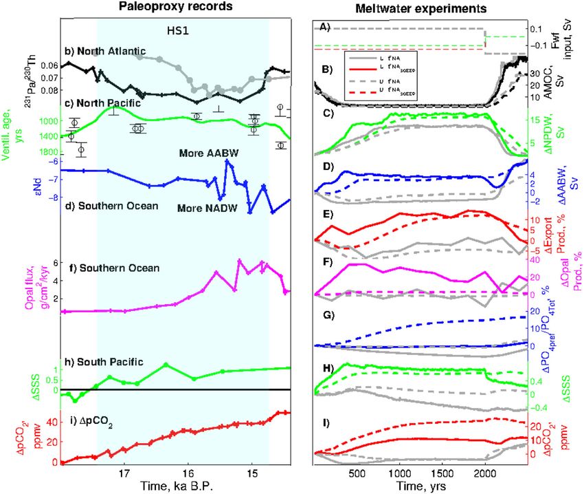
MENVIEL ET AL.: HEINRICH CO2

         Figure 5. DIC anomalies averaged over the Pacific basin and meridional overturning stream function:
         Latitude-depth DIC anomalies (mol/L) compared to the LGM control run, averaged over the Pacific
         basin for model years 1990–2000 for (top) standard meltwater experiments performed with (left) LOVE-
         CLIM and (right) the UVic ESCM, as well as (bottom) meltwater experiments with enhanced AABW
         transport. Overlaid are the meridional overturning stream function (Sv, black) integrated over the Indo-
         Pacific basin and the Ross Sea, as well as the South Pacific annual mean isopycnal surfaces (green)
         compared to the LGM control run (blue).

2.3. pCO2 Decomposition                                                  3. Results
  [10] The factors controlling surface water pCO2 and, ulti-             3.1. Idealized LGM Experiments
mately, atmospheric CO2 , include changes in SSS, SST,
dissolved inorganic carbon (DIC), and alkalinity (ALK)                      [13] The cessation of NADW formation under constant
[Sarmiento and Gruber, 2006; D’Orgeville et al., 2011]. We               LGM conditions in LOVECLIM and the UVic ESCM leads
use the following equations to decompose the pCO2 signal                 to an oceanic carbon reservoir increase and to a 4 ppmv
in Figure 2:                                                             atmospheric CO2 decrease (Table 1 and Figure 1I). Figure 2
                                                                         (d, blue and black lines) shows that the pCO2 decrease due
                                                                         to the AMOC shutdown may be partially attributed to the
 pCO2 = pCO2DIC + pCO2ALK + pCO2SST + pCO2SSS (1)
                                                                         enhanced CO2 solubility in seawater due to the global fresh-
                                                                         ening of the surface waters (Figure 2c, blue and black lines).
  [11] For DIC, ALK, and SSS:                                            The addition of freshwater into the North Atlantic to sim-
                                                                         ulate a shutdown of the AMOC leads to strong negative
                 pCO2X = X*X *pCO2Ref /X                   (2)        SSS anomalies across the entire Atlantic basin as well as
                                                                         throughout the Southern Ocean (Figure 3). A shutdown of
where X represents the mean DIC, ALK, or SSS value and                   the AMOC also leads to a classic SST seesaw response in
DIC , ALK , and SSS are equal to 10, –9.4, and 1, respectively        both LOVECLIM and the UVic ESCM, with a strong cool-
[Sarmiento and Gruber, 2006].                                            ing in the North Atlantic and warming in the Southern Ocean
  [12] The temperature contribution is derived from                      (Figure 4). The warming simulated over the Southern Ocean
                                                                         is, however, much greater in LOVECLIM than in the UVic
       pCO2SST = exp(SST*SST )*pCO2Ref – pCO2Ref           (3)        ESCM.
                                                                            [14] An increase in surface DIC leads to a greater oceanic
where SST is equal to 0.0423.                                           partial pressure of CO2 ; however, an increase in surface
                                                                    63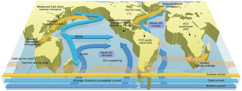
MENVIEL ET AL.: HEINRICH CO2

         Figure 6. Export production anomalies: Same as Figure 3 but for export production anomalies
         (gC/m2 /yr).

alkalinity decreases oceanic pCO2 . The imbalance between               [17] Even though quantitative SSS reconstructions are
changes in surface DIC and ALK explains a large part of              associated with large uncertainties [Legrande and Schmidt,
the atmospheric pCO2 decrease in the first 1000 years of the          2011], equatorial and South Pacific SSS most likely
experiments (Figures 2e and 2f). For example, in LOVE-               increased during Heinrich stadials 1 and 4 [Stott et al., 2002;
CLIM, the initial pCO2 decrease (500 years) is partly due           Pahnke et al., 2003; Calvo et al., 2007; Leduc et al., 2007],
to a low DIC anomaly in the surface waters, resulting from           in contradiction with our initial results (Figures 1h, 1H,
the greater stratification in the North Atlantic.                     and 3). It has been suggested that as the AMOC weakened,
  [15] Due to the weaker overturning in the Atlantic Ocean,          moisture transport from the Atlantic to the Pacific across
the residence time of deep waters increases, thus leading to         Central America was reduced [Richter and Xie, 2010] and
a greater DIC content in the deep Atlantic Ocean (200 GtC           that the East Asian Summer Monsoon weakened [Wang et
after 2000 yrs, Table 1). On the other hand, through oceanic         al., 2001]. These processes, best represented in multilevel
and atmospheric teleconnections a weak AMOC leads to the             high-resolution atmospheric General Circulation Models,
formation of NPDW [Saenko et al., 2004; Okazaki et al.,              would contribute to increased surface salinity in the Pacific
2010]. The greater ventilation of the North Pacific Ocean             Ocean, with significant consequences for Pacific deep and
(Figure 1C) leads to a loss of DIC in the North Pacific               bottom water formation. It is hypothesized that due to the
intermediate and deep waters (Table 1 and Figure 5).                 coarse resolution and simplified atmospheric physics of the
  [16] In agreement with previous studies [Schmittner,               models used in this study, the SSS in the Pacific Ocean might
2005; Obata, 2007; Chikamoto et al., 2012; Mariotti et al.,          be underestimated.
2012], reduced global and CaCO3 export production (up to                [18] We perform further Heinrich-type experiments in
–9%) are simulated in both models (Figures 1E, grey lines            which we try to rectify for the low surface salinity anoma-
and 6), mainly due to greater stratification over the Atlantic        lies in the Pacific Ocean. In experiments L-fNASOEEP and
region and to a weaker upwelling in the eastern Pacific               U-fNASOEEP , the surface salinity in the Southern Pacific
region (not shown). However, stratification further leads to          Ocean now increases by about 0.5 g/kg, consistent with pale-
a 6% and 12% increase in nutrient utilization efficiency              oproxy records for Heinrich stadials [Pahnke et al., 2003;
(1 – PO4surface /PO4deep ) in LOVECLIM and the UVic ESCM,            Calvo et al., 2007] (Figures 1h and 1H, green lines). Atmo-
respectively, thus enhancing the efficiency of the biological         spheric CO2 increases by respectively 10 and 25 ppmv
pump and effectively trapping carbon in the ocean interior.          in LOVECLIM and the UVic ESCM due to lower CO2
                                                                64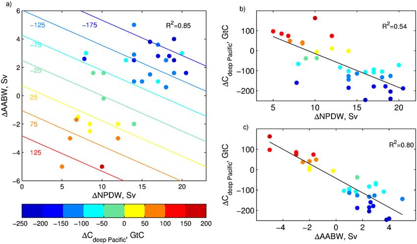
MENVIEL ET AL.: HEINRICH CO2
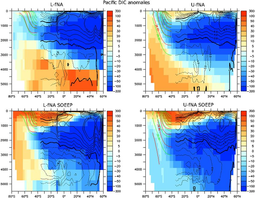
Figure 7. Sea-air pCO2 and mixed layer depth anomalies: Sea-air pCO2 anomalies (atm) for (top)
standard meltwater experiments and (bottom) for experiments in which the AABW and NPDW transport
strengthen, performed with (left) LOVECLIM and (right) the UVic ESCM. Contours indicate austral
winter mixed layer depth anomalies (m). Data shown correspond to the largest rate of pCO2 change: i.e.,
model years 190–200 and 390–400 for LOVECLIM, and 490–500 and 390–400 for the UVic ESCM. Red
colors represent CO2 outgassing into the atmosphere.
solubility as well as enhanced ventilation of the deep and component at certain longitudes and thus plays a role in
bottom waters of the Pacific Ocean (Figures 1 and 2). transporting heat poleward [Volkov et al., 2010]. In addition,
[19] During the AMOC shutdown, the surface waters get the East Australian Current and the Brazil Current strengthen
slightly saltier (0–0.2 g/kg) and warmer (0–0.4ı C), thus low- by 15% (not shown), thus bringing more warm and salty
ering CO2 solubility (Figures 2c and 2d, green and red lines). water to the South Pacific and South Atlantic.
In addition, the SSS increase leads to a strengthening of [20] The combination of strong AABW and NPDW leads
AABW in the Pacific Ocean by 3 to 5 Sv (Figure 1D, blue to enhanced ventilation of the Pacific basin (Figure 5). While
lines). AABW is calculated here as the maximum strength of the deep Atlantic basin is still a sink of carbon (Table 1),
the overturning in the abyssal cell at 35ı S. Stronger NPDW the transport of DIC-rich deep Pacific waters (Table 1 and
induces a warming at the surface of the North Pacific Ocean, Figure 5) to the surface and CO2 outgassing into the atmo-
particularly in its eastern part (Figure 4). As described else- sphere is thus significantly enhanced (Figure 7). The more
where [Saenko et al., 2004; Okazaki et al., 2010; Menviel saline surface waters (Figure 3) induce deep convection
et al., 2012b], formation of NPDW weakens the Indonesian primarily in the Pacific sector of the Southern Ocean as
throughflow transport while strengthening the Kuroshio Cur- indicated by the strong (up to 300 m) deepening of the
rent, thus enhancing the transport of warm tropical waters austral winter mixed layer depth (Figure 7) and a steep-
to the Northwest Pacific. A strengthening of AABW further ening of the isopycnals south of 50ı S (Figure 5). In the
enhances the warming at middle- and high-latitudes in the Pacific sector of the Southern Ocean, DIC is advected
Southern Hemisphere (Figure 4) via enhanced poleward heat equatorward by Ekman transport and CO2 outgassing thus
transport. In LOVECLIM, enhanced AABW strengthens occurs south of 58ı S. In LOVECLIM, the DIC-rich waters
the ACC by 15% (not shown). The Antarctic Circumpo- are also transported by the ACC to the South Atlantic
lar Current (ACC) is not only zonal but has a meridional and the South Indian Oceans, where the CO2 flux to the
65MENVIEL ET AL.: HEINRICH CO2
Figure 8. Relation between deep Pacific carbon, Antarctic Bottom Water, and North Pacific Deep Water:
(a) Deep Pacific carbon content anomalies (GtC, 2000m for LOVECLIM and 2200m for the UVic
ESCM) as a function of the change in Antarctic Bottom Water (AABW, Sv) and North Pacific Deep Water
(NPDW, Sv). The stronger AABW and NPDW are, the more carbon is ventilated out of the Pacific Ocean.
(b) Deep Pacific carbon content anomalies (GtC) as a function of the change in NPDW (Sv). (c) Deep
Pacific carbon content anomalies (GtC) as a function of the change in AABW (Sv). Each point represents
the result of a sensitivity experiment for model years 990–1000 (Tables S2 and S3). The multiple linear
regression analysis of deep Pacific carbon content anomalies versus change in AABW and NPDW leads
to a correlation coefficient, R2 , of 0.85. Most of the variability is due to changes in AABW (R2 =0.80). In
Figure 8a, the colored contour lines indicate values obtained if the linear relationship held perfectly.
atmosphere is enhanced at 40ı S–50ı S. In the UVic ESCM, increase in the preformed phosphate (PO4Pref ) inventory [Ito
the ACC transport is weaker than in LOVECLIM and and Follows, 2005]. Here we argue that these variations
the Southern Ocean SST (Figure 4) does not increase in PO4Pref are mainly due to changes in the ventilation of
as much; therefore, all the CO2 outgassing occurs in the the Pacific bottom and deep water masses, i.e., enhanced
Pacific Ocean. AABW and to a lesser extent enhanced NPDW transport.
[21] In LOVECLIM, greater ventilation of the Southern In LOVECLIM, changes in atmospheric CO2 content also
Ocean enhances opal production over the South Atlantic reflect changes in AABW and NPDW transport; however,
Ocean, in good agreement with a record from the South there is no clear link with changes in PO4Pref inventory. This
Atlantic (Figures 1f and 1F, magenta lines) [Anderson et al., is partly due to the small PO4Pref gradient in the deep Atlantic
2009]. The global export production also now increases by basin under LGM conditions. In addition, as already shown
10–15% in both models (Figure 1E, red lines). in Menviel et al. [2008b], the biological pump in the South-
[22] It should be noted that in the UVic ESCM, once the ern Ocean is very reactive in LOVECLIM. The enhanced
AMOC is shut down it does not recover without the addition Southern Ocean ventilation leads to a 30% increase in
of a negative buoyancy flux over the North Atlantic Ocean export production over the Southern Ocean in LOVECLIM,
(e.g., freshwater extraction from the ocean). Instead, NPDW whereas Southern Ocean export production decreases by 7%
formation strengthens and after the freshwater forcing in the in the UVic ESCM (Figure 6).
North Atlantic has stopped, the surface salinity of the Pacific [23] Figures 2e and 2f show the different contributions of
Ocean increases, thus leading to a strengthening of AABW DIC and ALK to the pCO2 change. The individual contri-
formation. For example, in experiments performed with the butions of DIC and ALK are larger in LOVECLIM than in
UVic ESCM and forced with a 0.2 Sv freshwater input in the UVic ESCM, due to the greater gradient of both DIC
the North Atlantic for 500 years (see supporting informa- and ALK between the surface and the deep (not shown). The
tion), the AABW transport first weakens by 1.8 Sv then resulting pCO2 anomalies, however, depend on the relative
slowly increases up to 2 Sv compared to the initial state. As contribution of DIC over alkalinity. The imbalance between
a result atmospheric CO2 first decreases by 5 ppmv and then alkalinity and DIC is much larger for the UVic ESCM thus
increases in phase with AABW to reach a pCO2 anomaly contributing to about 18 ppmv pCO2 increase. This is mainly
of +5 ppmv. This result is similar to the one obtained by due to the much greater DIC gradient between the surface
Schmittner et al. [2007]; however, it is lower than the 22 and the deep compared to the vertical alkalinity gradient
ppmv atmospheric CO2 increase simulated by Schmittner (not shown). DIC and alkalinity gradients are set by the
and Galbraith [2008] under the same forcing conditions. biological and carbonate pumps in the ocean thus indicat-
Schmittner and Galbraith [2008] show that the atmospheric ing stronger biological and carbonate pumps in LOVECLIM
CO2 rise simulated in their experiments was due to the global than in the UVic ESCM.
66MENVIEL ET AL.: HEINRICH CO2
3.2. Changes in AABW and NPDW and Their Impact
on Deep Pacific Carbon
[24] Our results highlight the importance of changes in
AABW and NPDW and their impact on oceanic and atmo-
spheric carbon. Depending on the bottom and deep water
mass transports in the Pacific Ocean, the ocean can act either
as a sink or as a source of carbon through an Atlantic-Pacific
seesaw. The stronger the transport of NPDW and AABW
in the Pacific Ocean, the more carbon is released from
the deep Pacific through the Southern Ocean to the atmo-
sphere. Figure 8 shows the relationship between changes in
deep Pacific carbon, AABW and NPDW transport obtained
from a series of sensitivity experiments (LOVECLIM and
the UVic ESCM, including different freshwater forcing and
Gent McWilliams parametrization coefficients, Tables S1
and S3.)
[25] Deep Pacific carbon release primarily depends on
AABW transport, as indicated by a 0.80 correlation coeffi-
cient between these two model integral metrics. A multilin-
ear regression analysis including both AABW and NPDW
slightly improves the correlation (R2 =0.85), thus corrob-
orating the role of stronger NPDW in outgassing CO2 .
However, this regression underestimates the role of NPDW
as it only takes into account changes in carbon below 2000
m depth. Stronger NPDW ventilates North Pacific interme-
diate waters and is thus a main factor in controlling the
Pacific carbon budget (Figure 5). This is also confirmed
by the results of meltwater experiments performed with
the coupled Atmospheric Ocean General Circulation model
MIROC 3.2 [Chikamoto et al., 2012], in which atmospheric Figure 9. Model-paleoproxy comparison for Heinrich sta-
CO2 decreases by 15 ppmv. The atmospheric CO2 decrease dial 4: Results of transient experiments L-HS4 (black) and
is partly due to the enhanced CO2 solubility due to colder L-HS4SOEEP (blue) compared to paleoproxy records (red).
and fresher surface waters. In addition, the NPDW transport Time series of (a) Maximum overturning circulation in the
is negligible so that carbon can be stored in both the Atlantic North Atlantic (Sv) (blue) as well as freshwater forcing (Sv)
and Pacific Oceans. in the North Atlantic for both experiments (black) and over
the Southern Ocean and the EEP for L-HS4SOEEP (dashed
3.3. Validation of the Mechanism for Heinrich Stadial 4 blue); (b) Changes in sea level (m) resulting from the forc-
[26] We now run a fully coupled transient simulation of ing applied compared to the estimates from the Red Sea
HS4 from 40.5 to 38.5 ka B.P. forcing LOVECLIM with (red) [Siddall et al., 2003] and from Papua New Guinea
a freshwater input in the North Atlantic (Figure 9, black (magenta) [Chappell, 2002]; (c) Greenland air temperature
lines). A shutdown of the AMOC during HS4 leads to sim- (ı C) as simulated and as recorded in the North Greenland Ice
ulated air temperature and SST anomalies over Greenland Core Project (NGRIP) ice core [Huber et al., 2006]; (d) SST
and the Iberian margin in reasonable agreement with pale- anomalies (ı C) as simulated and as recorded in marine sedi-
oproxy records [Huber et al., 2006; Bard, 2002; Martrat et ment core MD95-2042 off the Iberian margin [Martrat et al.,
al., 2007; Elliot et al., 2002; Cacho et al., 1999]. However, 2007]; (e) SSS anomaly in the South Pacific Ocean (175ı E–
the simulated SSS over the Eastern Equatorial Pacific (EEP) 260ı E, 35ı S–48ı S) compared to the SSS anomaly estimated
and the Southern Ocean decrease by 0.4 g/kg and there is from ı 18 O and SST from marine sediment core MD97-
no significant atmospheric CO2 increase simulated between 2120 [Pahnke et al., 2003]; (f) opal production anomaly
39.75 and 39.4 ka B.P. (%) averaged over the South Atlantic Ocean (50ı W–20ı E,
[27] We run an additional fully coupled transient simula- 42ı S–60ı S) compared to the opal flux anomaly (%) record
tion of HS4, which includes a freshwater flux in the North from the South Atlantic marine sediment core TNO57-14PC
Atlantic and a salt flux over the Southern Ocean, and the [Anderson et al., 2009]; (g) atmospheric CO2 (ppmv) as
EEP to compensate for the low salinity anomaly over the simulated and as recorded in Byrd ice core, Antarctica
Pacific Ocean, equivalent to the experiments described in [Ahn and Brook, 2008].
section 3.1. In this new experiment, the forcing is equivalent
to a 12 m sea level rise, compared to the 20 m sea level rise Southern Ocean increases by 2.0 and 0.6 g/kg, respectively,
in the first experiment. The forcing applied in both experi- in better agreement with paleoproxy records [Leduc et al.,
ments is consistent with sea level rise estimates of 10–25 m 2007; Pahnke et al., 2003]. In addition, the opal produc-
for HS4 [Chappell, 2002; Siddall et al., 2003]. The agree- tion in the Southern Ocean increases significantly (+25%),
ment between modeling results and paleoproxies is still good consistent with a proxy record from the South Atlantic
over Greenland and the North Atlantic (Figure 9, blue lines). [Anderson et al., 2009]. Saltier surface conditions over
Notably, in the new experiment, the SSS in the EEP and the the Southern and North Pacific Oceans lead to enhanced
67MENVIEL ET AL.: HEINRICH CO2
Figure 10. Mechanism for CO2 release during Heinrich stadials 4 and 1: A shutdown of the AMOC
leads to a greater heat transport to the south and a sea ice retreat in the Southern Ocean. The North Atlantic
cooling induces a southward shift of the Intertropical Convergence Zone, a weakening of the East Asian
Summer Monsoon and a reduced moisture transport from the Atlantic to the Pacific over Central America.
Due to an increased salinity at the surface of the Pacific Ocean, the transport of AABW and NPDW is
enhanced, thus effectively releasing deep Pacific carbon into the atmosphere through the Southern Ocean.
The deep carbon reservoir is reduced in the Pacific, while it increases in the Atlantic Ocean.
formation and transport of NPDW and AABW in the Xie, 2010; Peterson et al., 2000] (Figure 10). A weaker East
Pacific Ocean, thus effectively ventilating deep Pacific car- Asian Summer monsoon [Tada et al., 1999; Wang et al.,
bon through the Southern Ocean. We simulate a 10 ppmv 2001] also increases the salinity in the North Pacific. Finally,
atmospheric CO2 increase over 300 years, close to the 15 it has been suggested that a stronger Kuroshio Current cou-
ppmv atmospheric CO2 rise observed in the Byrd ice core pled to a reduced Indonesian throughflow could lead to the
[Ahn and Brook, 2008; Ahn et al., 2012]. Our results sug- formation of NPDW [Okazaki et al., 2010]. Through the
gest that enhanced deep and bottom water mass transport in Stommel feedback [Stommel, 1961], the NPDW strength-
the Pacific Ocean could have played a critical role in raising ening leads to an increase in the salinity of North Pacific
atmospheric CO2 during HS4. waters. In the Southern Ocean, the increased heat flux due
to the AMOC weakening and the strong Southern Hemi-
4. Discussion and Conclusions spheric high-latitude insolation results in a sea ice retreat. In
addition, positive salinity anomalies that arise in the East-
[28] Our results show that solubility effects as well as ern Equatorial Pacific can be advected to the South Pacific
changes in the deep and bottom water mass transport in the and across the ACC by eddies. We hypothesize that the sea
Pacific Ocean are the primary control of the marine carbon ice retreat associated with greater surface salinity induces
cycle during a shutdown of the Atlantic Meridional Over- deep convection around 60ı S primarily in the Pacific sector
turning Circulation (AMOC). Depending on the strength of of the Southern Ocean [Meissner et al., 2008], thus releas-
Antarctic Bottom Water (AABW) and North Pacific Deep ing carbon stored in the deep Pacific Ocean. Both deep
Water (NPDW), the ocean can act either as a sink or as a convection and rising atmospheric CO2 provide a positive
source of carbon through an Atlantic-Pacific seesaw. The feedback, further enhancing the sea ice retreat. A reduction
stronger the transport of NPDW and AABW in the Pacific in the density gradient between the North and South Pacific
Ocean, the more carbon is released from the deep and inter- could also enhance the AABW transport in the Pacific Ocean
mediate Pacific to the atmosphere. In addition, changes in [Watson and Naveira Garabato, 2006]. Such a mechanism
NPDW and AABW have an influence on the climate of the (Figure 10) operating during HS4 is consistent with paleo-
Pacific region [Menviel et al., 2010, 2012b] and are thus also proxy records as it induces a carbonate ion rise in the deep
important for changes in terrestrial carbon. Indian and Pacific Oceans [Yu et al., 2010, 2013], increases
[29] Our fully coupled transient simulation of HS4 has surface salinity in the Pacific Ocean [Leduc et al., 2007;
further shown that an increase in AABW and NPDW trans- Pahnke et al., 2003], enhances AABW transport [Piotrowski
port during the AMOC shutdown could have played a major et al., 2005], and leads to greater upwelling of nutrient-
role in shaping the observed atmospheric CO2 increase rich waters in the Southern Ocean (Figure 9) [Anderson et
(Figure 9) [Ahn and Brook, 2008]. Around 40 ka B.P., the al., 2009], thus effectively increasing atmospheric CO2 [Ahn
Antarctic ice sheet was close to its maximum extent and and Brook, 2008].
presumably covered most of present-day AABW formation [30] A similar mechanism occurring during HS1 is also
regions: the Weddell and Ross Seas [Denton and Hughes, consistent with paleoproxy records as it lowers atmo-
2002; Pollard and DeConto, 2009]. At the onset of HS4, spheric ı 13 CO2 [Schmitt et al., 2012; Tschumi et al., 2011],
meltwater in the North Atlantic slows down NADW forma- decreases the ventilation age of deep Southern Ocean waters
tion. Reduced moisture transport from the Atlantic to the [Skinner et al., 2010], and enhances mixing of Upper and
Pacific across Central America increases the salinity in the Lower Circumpolar Deep Waters [Burke and Robinson,
Eastern Equatorial Pacific [Leduc et al., 2007; Richter and 2012]. It is also consistent with a decrease in atmospheric
68MENVIEL ET AL.: HEINRICH CO2
14 C [Huiskamp and Meissner, 2012; Matsumoto and Chappell, J. (2002), Sea level changes forced ice breakouts in the last glacial
Yokoyama, 2013]. Antarctic ice cores record an atmospheric cycle: New results from coral terraces, Quat. Sci. Rev., 21, 1229–1240.
Chikamoto, M. O., L. Menviel, A. Abe-Ouchi, R. Ohgaito, A.
CO2 increase of 33 ppmv at the beginning of the last Timmermann, Y. Okazaki, N. Harada, A. Oka, and A. Mouchet (2012),
deglaciation and across HS1 [Monnin et al., 2001]. Our Variability in North Pacific intermediate and deep water ventilation dur-
results suggest that enhanced AABW and NPDW trans- ing Heinrich events in two coupled climate models, Deep Sea Res. Part
II, 61–64, 114–126.
port during HS1 could have accounted for about 30% of Condron, A., and P. Winsor (2011), A subtropical fate awaited freshwater
the observed atmospheric CO2 increase. Such an atmo- discharged from glacial Lake Agassiz, Geophys. Res. Lett., 38, L03705,
spheric pCO2 increase during HS1 would contribute to the doi:10.1029/2010GL046011.
last deglaciation atmospheric pCO2 increase alongside other Dansgaard, W., S. J. Johnsen, and H. B. Clausen (1993), Evidence for gen-
eral instability of past climate from a 250-kyr ice-core record, Nature,
mechanisms [Menviel et al., 2012a]. 364, 218–220.
[31] Our study suggests that an AMOC shutdown associ- Denton, G. H., and T. J. Hughes (2002), Reconstructing the Antarctic Ice
ated with a strengthening of the Pacific AABW and NPDW Sheet at the Last Glacial Maximum, Quat. Sci. Rev., 21, 193–202.
during HS4 and possibly HS1 led to a release of carbon Deplazes, G., et al. (2013), Links between tropical rainfall and North
Atlantic climate during the last glacial period, Nat. Geosci., 6, 213–217,
into the atmosphere in agreement with paleoproxy records. doi:10.1038/NGEO1712.
Depending on the background conditions and the magnitude D’Orgeville, M., M. H. England, and W. P. Sijp (2011), Buffered versus
of the event, not all Heinrich stadials might be associated non-buffered ocean carbon reservoir variations: Application to the sen-
sitivity of atmospheric CO2 to ocean circulation changes, Geophys. Res.
with enhanced AABW transport. This could explain the Lett., 38, L24603, doi:10.1029/2011GL049823.
lack of noticeable atmospheric CO2 increase during HS2, Elliot, M., L. Labeyrie, G. Bond, E. Cortijo, J.-L. Turon, N. Tisnerat, and
for example. J.-C. Duplessy (1998), Millennial-scale iceberg discharges in the
Irminger Basin during the last glacial period: Relationship with the
Heinrich events and the environmental settings, Paleoceanography, 13,
[32] Acknowledgments. This project was supported by the Australian 433–446.
Research Council. Model experiments were performed on a computa- Elliot, M., L. Labeyrie, and J.-C. Duplessy (2002), Changes in North
tional cluster owned by the Faculty of Science of the University of New Atlantic deep-water formation associated with the Dansgaard-Oeschger
South Wales as well as on a cluster from the NCI National Facility at the temperature oscillations (60-10 ka), Quat. Sci. Rev., 21, 1153–1165.
Australian National University. K.J. Meissner acknowledges funding from Gherardi, J. M., L. Labeyrie, J. F. McManus, R. Francois, L. C.
the ARC Future Fellowship program (FT100100443) and M. England fund- Skinner, and E. Cortijo (2005), Evidence from the Northeastern Atlantic
ing from the ARC Laureate Fellowship program (FL100100214). We thank basin for variability in the rate of the meridional overturning cir-
Editor H. Päelike and A. Schmittner, as well as an anonymous reviewer for culation through the last deglaciation, Earth Planet. Sci. Lett., 240,
their constructive comments. 710–723.
Goosse, H., et al. (2010), Description of the Earth system model of inter-
mediate complexity LOVECLIM version 1.2, Geosci. Model Dev., 3,
603–633.
References Grousset, F. E., C. Pujol, L. Labeyrie, G. Auffret, and A. Boelaert (2000),
Abe-Ouchi, A., T. Segawa, and F. Saito (2007), Climatic conditions for Were the North Atlantic Heinrich events triggered by the behavior of the
modelling the Northern Hemisphere ice sheets throughout the Ice Age European ice sheets?, Geology, 28, 123–126.
cycle, Clim. Past, 3, 423–438. Heinrich, H. (1988), Origin and consequences of cyclic ice rafting in the
Ahn, J., and E. J. Brook (2008), Atmospheric CO2 and climate on mil- northeast Atlantic Ocean during the past 130,000 years, Quat. Res., 29,
lennial time scales during the last glacial period, Science, 322, 83–85, 142–152.
doi:10.1126/science.1160832. Hemming, S. R. (2004), Heinrich events: Massive late Pleistocene detri-
Ahn, J., E. J. Brook, A. Schmittner, and K. J. Kreutz (2012), Abrupt change tus layers of the North Atlantic and their global climate imprint, Rev.
in atmospheric CO2 during the last ice age, Geophys. Res. Lett., 39, Geophys., 42, RG1005, doi:10.1029/2003RG000128.
L18711, doi:10.1029/2012GL053018. Huber, C., M. Leuenberger, R. Spahni, J. Flückiger, J. Schwander, T. F.
Anderson, R. F., S. Ali, L. I. Bradtmiller, S. H. H. Nielsen, M. Q. Fleisher, Stocker, S. Johnsen, A. Landais, and J. Jouzel (2006), Isotope cali-
B. E. Anderson, and L. H. Burckle (2009), Wind-driven upwelling in the brated Greenland temperature record over Marine Isotope Stage 3 and its
Southern Ocean and the deglacial rise in Atmospheric CO2 , Science, 323, relation to CH4, Earth Planet. Sci. Lett., 243, 504–519.
1443–1448. Huiskamp, W. N., and K. J. Meissner (2012), Oceanic carbon and water
Bard, E. (2002), Abrupt climate changes over millennial time scales: masses during the Mystery Interval: A model-data comparison study,
Climate shock, Phys. Today, 55, 32–38. Paleoceanography, 27, PA4206, doi:10.1029/2012PA002368.
Bereiter, B., D. Lüthi, M. Siegrist, S. Schüpbach, T. F. Stocker, and H. Ito, T., and M. J. Follows (2005), Preformed phosphate, soft tissue pump
Fischer (2012), Mode of change of millennial CO2 variability during the and atmospheric CO2 , J. Mar. Res., 63, 813–839.
last glacial cycle associated with a bipolar marine carbon seesaw, Proc. Köhler, P., F. Joos, S. Gerber, and R. Knutti (2005), Simulated changes
Natl. Acad. Sci., 109, 9755–9760, doi:10.1073/pnas.1204069109. in vegetation distribution, land carbon storage, and atmospheric CO2 in
Berger, A. (1978), Long term variations of daily insolation and Quaternary response to a collapse of the North Atlantic thermohaline circulation,
climate change, J. Atmos. Sci., 35, 2362–2367. Clim. Dyn., 25, 689–708.
Blunier, T., and E. J. Brook (2001), Timing of millennial-scale climate Leduc, G., L. Vidal, K. Tachikawa, F. Rostek, C. Sonzogni, L. Beaufort, and
change in Antarctica and Greenland during the last glacial period, E. Bard (2007), Moisture transport across Central America as a positive
Science, 291, 109–112. feedback on abrupt climatic changes, Nature, 445, 908–911.
Bond, G. (1993), Correlations between climate records from North Atlantic Legrande, A., and G. A. Schmidt (2011), Water isotopologues as
sediments and Greenland ice, Nature, 365, 143–147. a quantitative paleosalinity proxy, Paleoceanography, 26, PA3225,
Bouttes, N., D. M. Roche, and D. Paillard (2012), Systematic study of the doi:10.1029/2010PA002043.
impact of fresh water fluxes on the glacial carbon cycle, Clim. Past, 8, Lisiecki, L. E., M. E. Raymo, and W. B. Curry (2008), Atlantic overturning
589–607. responses to Late Pleistocene climate forcings, Nature, 456, 85–88.
Bozbiyik, A., M. Steinacher, F. Joos, T. F. Stocker, and L. Menviel (2011), Marchal, O., T. F. Stocker, F. Joos, A. Indermühle, T. Blunier, and J.
Fingerprints of changes in the terrestrial carbon cycle in response to large Tschumi (1999), Modelling the concentration of atmospheric CO2 during
reorganizations in ocean circulation, Clim. Past, 7, 319–338. the Younger Dryas climate event, Clim. Dyn, 15, 341–354.
Burke, A., and L. F. Robinson (2012), The Southern Ocean’s role in carbon Mariotti, V., L. Bopp, A. Tagliabue, M. Kageyama, and D. Swingedouw
exchange during the last deglaciation, Science, 335, 557–561. (2012), Marine productivity response to Heinrich events: A model-data
Cacho, I., J. O. Grimalt, C. Pelejero, M. Canals, F. J. Sierro, J. A. Flores, and comparison, Clim. Past, 8, 1581–1598.
N. Shackleton (1999), Dansgaard-Oeschger and Heinrich event imprints Martrat, B., J. O. Grimalt, N. J. Shackleton, L. de Abreu, M. A. Hutterli, and
in Alboran Sea paleotemperatures, Paleoceanography, 14, 698–705. T. F. Stocker (2007), Four climate cycles of recurring deep and surface
Calvo, E., C. Pelejero, P. De Deckker, and G. A. Logan (2007), water destabilizations on the Iberian margin, Science, 317, 502–507.
Antarctic deglacial pattern in a 30 kyr record of sea surface tem- Matsumoto, K., and Y. Yokoyama (2013), Atmospheric 14 C reduction
perature offshore South Australia, Geophys. Res. Lett., 34, L13707, in simulations of Atlantic overturning circulation shutdown, Global
doi:10.1029/2007GL029937. Biogeochem. Cycles, 27, 296–304, doi:10.1002/gbc.20035.
69MENVIEL ET AL.: HEINRICH CO2
McManus, J. F., R. Francois, J. M. Gherardi, L. D. Keigwin, and S. Sarmiento, J. L., and N. Gruber (2006), Ocean Biogeochemical Dynamics,
Brown-Leger (2004), Collapse and rapid resumption of Atlantic merid- pp. 526, Princeton Univ. Press, Princeton, N. J.
ional circulation linked to deglacial climate changes, Nature, 428, Schmidt, G. A., G. R. Bigg, and E. J. Rohling (1999), Global Seawater
834–837. Oxygen-18 Database, v1.21. http://data.giss.nasa.gov/o18data/.
Meissner, K. J., A. Schmittner, A. J. Weaver, and J. F. Adkins (2003a), The Schmitt, J., et al. (2012), Carbon isotope constraints on the deglacial CO2
ventilation of the North Atlantic Ocean during the Last Glacial Maxi- rise from ice cores, Science, 136, 711–714.
mum: A comparison between simulated and observed radiocarbon ages, Schmittner, A. (2005), Decline of the marine ecosystem caused by a
Paleoceanography, 18(2), 1023, doi:10.1029/2002PA000762. reduction in the Atlantic overturning circulation, Nature, 434, 628–633.
Meissner, K. J., A. J. Weaver, H. D. Matthews, and P. M. Cox (2003b), The Schmittner, A., and E. D. Galbraith (2008), Glacial greenhouse-gas
role of land surface dynamics in glacial inception: A study with the UVic fluctuations controlled by ocean circulation changes, Nature, 456,
Earth System Model, Clim. Dyn., 21, 515–537. 373–376.
Meissner, K. J., M. Eby, A. J. Weaver, and O. A. Saenko (2008), CO2 Schmittner, A., E. J. Brook, and J. Ahn (2007), Impact of the ocean’s
threshold for millennial-scale oscillations in the climate system: Implica- overturning circulation on atmospheric CO2, in Ocean Circulation:
tions for global warming scenarios, Clim. Dyn., 30, 161–174. Mechanisms and Impacts, Geophys. Monogr. Ser., vol. 173, edited by A.
Meissner, K. J., B. I. McNeil, M. Eby, and E. C. Wiebe (2012), The Schmittner, J. C. H. Chiang, and S. R. Hemming, pp. 315–334, AGU,
importance of the terrestrial weathering feedback for multimillennial Washington, D. C.
coral reef habitat recovery, Global Biogeochem. Cycles, 26, GB3017, Schmittner, A., A. Oschlies, H. D. Matthews, and E. D. Galbraith (2008),
doi:10.1029/2011GB004098. Future changes in climate, ocean circulation, ecosystems, and bio-
Menviel, L. (2008), Climate-carbon cycle interactions on millennial to geochemical cycling simulated for a business-as-usual CO2 emission
glacial timescales as simulated by a model of intermediate complexity, scenario until year 4000 AD, Global Biogeochem. Cycles, 22, GB1013,
LOVECLIM, PhD thesis, University of Hawai’i, http://myweb.science. doi:10.1029/2007GB002953.
unsw.edu.au/lauriemenviel/Menvielthesis2008.pdf. Scholze, M., W. Knorr, and M. Heimann (2003), Modelling terrestrial veg-
Menviel, L., A. Timmermann, A. Mouchet, and O. Timm (2008a), etation dynamics and carbon cycling for an abrupt climatic change event,
Meridional reorganizations of marine and terrestrial produc- Holocene, 13, 327–333.
tivity during Heinrich events, Paleoceanography, 23, PA1203, Shackleton, N. J. (1974), Les methodes quantitatives d’etude des variations
doi:10.1029/2007PA001445. du climat au cours du Pleistocene, vol. 219, Editions du Centre national
Menviel, L., A. Timmermann, A. Mouchet, and O. Timm (2008b), Cli- de la recherche scientifique (CNRS), Paris.
mate and marine carbon cycle response to changes in the strength of Siddall, M., E. J. Rohling, A. Almogi-Labin, C. Hemleben, D. Meischner,
the southern hemispheric westerlies, Paleoceanography, 23, PA4201, I. Schmelzer, and D. A. Smeed (2003), Sea-level fluctuations during the
doi:10.1029/2007PA001604. last glacial cycle, Nature, 423, 853–858.
Menviel, L., A. Timmermann, A. Mouchet, and O. Timm (2010), Climate Skinner, L. C., S. Fallon, C. Waelbroeck, E. Michel, and S. Barker (2010),
and biogeochemical response to a rapid melting of the West-Antarctic Ventilation of the deep Southern Ocean and deglacial CO2 rise, Science,
Ice Sheet during interglacials and implications for future climate, 328, 1147–1151.
Paleoceanography, 25, PA4231, doi:10.1029/2009PA001892. Snoeckx, H., F. Grousset, M. Revel, and A. Boelaert (1999), European con-
Menviel, L., F. Joos, and S. P. Ritz (2012a), Modeling atmospheric CO2 , tribution of ice-rafted sand to Heinrich layers H3 and H4, Mar. Geol.,
stable carbon isotope and marine carbon cycle changes during the last 158, 197–208.
glacial-interglacial cycle, Quat. Sci. Rev, 56, 46–68. Spence, P., O. A. Saenko, W. Sijp, and M. H. England (2013),
Menviel, L., A. Timmermann, A. Mouchet, O. Timm, A. Abe-Ouchi, M. O. North Atlantic climate response to Lake Agassiz drainage at coarse
Chikamoto, N. Harada, R. Ohgaito, and Y. Okazaki (2012b), Removing and ocean eddy-permitting resolutions, J. Climate, 26, 2651–2667,
the North Pacific halocline: Effects on global climate, ocean circulation doi:10.1175/JCLI–D–11–00683.1.
and the carbon cycle, Deep Sea Res. Part II, 61-64, 106–113. Stommel, H. M. (1961), Thermohaline convection with two stable regimes
Menviel, L., A. Timmermann, T. Friedrich, and M. H. England (2013), of flow, Tellus, 13, 224–230.
Hindcasting the continuum of Dansgaard-Oeschger variability: Mecha- Stott, L. C., C. Poulsen, S. Lund, and R. Thunell (2002), Super ENSO
nisms, patterns and timing, Clim. Past Discuss., 9, 4771–4806. and global climate oscillations at millenial time scales, Science, 279,
Monnin, E., A. Indermühle, A. Dällenbach, J. Flückiger, B. Stauffer, 222–226.
T. F. Stocker, D. Raynaud, and J.-M. Barnola (2001), Atmospheric CO2 Tada, R., T. Irino, and I. Koizumi (1999), Land-ocean linkages over orbital
concentration over the last glacial termination, Science, 291, 112–114. and millennial time-scales recorded in late Quaternary sediments of the
Mouchet, A. (2011), A 3D model of ocean biogeochemical cycles and cli- Japan Sea, Paleoceanography, 14, 236–247.
mate sensitivity studies, PhD thesis, Université de Liège, Lìege, Belgium, Tschumi, T., F. Joos, M. Gehlen, and C. Heinze (2011), Deep ocean venti-
http://hdl.handle.net/2268/98995. lation, carbon isotopes, marine sedimentation and the deglacial CO2 rise,
Obata, A. (2007), Climate-carbon cycle model response to freshwater Clim. Past, 7, 771–800.
discharge into the North Atlantic, J. Clim., 20, 5962–5976. Vidal, L., L. Labeyrie, E. Cortijo, M. Arnold, J. C. Duplessy, E. Michel,
Okazaki, Y., A. Timmermann, L. Menviel, N. Harada, A. Abe-Ouchi, M. S. Becque, and T. C. E. van Weering (1997), Evidence for changes in
Chikamoto, A. Mouchet, and H. Asahi (2010), Deep water formation the North Atlantic Deep Water linked to meltwater surges during the
in the North Pacific during the Last Glacial termination, Science, 329, Heinrich events, Earth Planet. Sci. Lett., 146, 13–27.
200–204. Volkov, D. L., L.-L. Fu, and T. Lee (2010), Mechanisms of the meridional
Pahnke, K., R. Zahn, H. Elderfield, and M. Schulz (2003), 340,000- heat transport in the Southern Ocean, Ocean Dyn., 60, 791–801.
year centennial-scale marine record of Southern Hemisphere climatic Waelbroeck, C., L. Labeyrie, J.-C. Duplessy, J. F. McManus, K. Lambeck,
oscillation, 301, 948–952. E. Balbon, and M. Labracherie (2002), Sea-level and deep water temper-
Parrenin, F., V. Masson-Delmotte, P. Köhler, D. Raynaud, D. Paillard, J. ature changes derived from benthic foraminifera isotopic records, Quat.
Schwander, C. Barbante, A. Landais, A. Wegner, and J. Jouzel (2013), Sci. Rev., 21, 295–305.
Synchronous change of atmospheric CO2 and Antarctic temperature Wang, Y. J., H. Cheng, R. L. Edwards, Z. S. An, J. Y. Wu, C. C. Shen, and
during the last deglacial warming, Science, 339, 1060–1063. J. A. Dorale (2001), A high-resolution absolute-dated Late Pleistocene
Peterson, L. C., G. H. Haug, K. A. Hughen, and U. Rohl (2000), Rapid monsoon record from Hulu Cave, China, Science, 294, 2345–2348.
changes in the hydrologic cycle of the Tropical Atlantic during the Last Watson, A. J., and A. C. Naveira Garabato (2006), The role of Southern
Glacial, Science, 290, 1947–1951. Ocean mixing and upwelling in glacial-interglacial atmospheric CO2
Piotrowski, A. M., S. L. Goldstein, S. R. Hemming, and R. G. Fairbanks change, Tellus B, 58, 73–87.
(2005), Temporal relationships of carbon cycling and ocean circulation Weaver, A. J., et al. (2001), The UVic Earth System Climate Model: Model
glacial boundaries, Science, 307, 1933–1938. description, climatology, and applications to past, present and future
Pollard, D., and R. M. DeConto (2009), Modelling West Antarctic ice sheet climates, Atmos. Ocean, 4, 361–428.
growth and collapse through the past five million years, Nature, 458, Yu, J., W. S. Broecker, H. Elderfield, Z. Jin, J. McManus, and F. Zhang
329–332. (2010), Loss of carbon from the deep sea since the Last Glacial Maxi-
Richter, I., and S.-P. Xie (2010), Moisture transport from the Atlantic to mum, Science, 330, 1084–1087.
the Pacific basin and its response to North Atlantic cooling and global Yu, J., R. F. Anderson, Z. Jin, J. W. B. Rae, B. N. Opdyke, and S. M. Eggins
warming, Clim. Dyn., 35, 551–566. (2013), Responses of the deep ocean carbonate system to carbon reor-
Saenko, O. A., A. Schmittner, and A. J. Weaver (2004), The Atlantic-Pacific ganization during the Last Glacial-interglacial cycle, Quat. Sci. Rev., 76,
seesaw, J. Climate, 17, 2033–2038. 39–52.
70You can also read