Optimized One-Click Development for Topology-Optimized Structures - MDPI
←
→
Page content transcription
If your browser does not render page correctly, please read the page content below
applied
              sciences
Article
Optimized One-Click Development for Topology-
Optimized Structures †
Tobias Rosnitschek * , Rick Hentschel, Tobias Siegel, Claudia Kleinschrodt, Markus Zimmermann,
Bettina Alber-Laukant and Frank Rieg

                                          Engineering Design and CAD, University of Bayreuth, Universitaetsstr. 30, 95447 Bayreuth, Germany;
                                          rick.hentschel@uni-bayreuth.de (R.H.); tobias.siegel@uni-bayreuth.de (T.S.);
                                          claudia.kleinschrodt@uni-bayreuth.de (C.K.); markus.zimmermann@uni-bayreuth.de (M.Z.);
                                          bettina.alber@uni-bayreuth.de (B.A.-L.); frank.rieg@uni-bayreuth.de (F.R.)
                                          * Correspondence: tobias.rosnitschek@uni-bayreuth.de
                                          † The presented “One-Click Development” is incorporated into the freeware Z88Arion®and can be used to
                                             develop lightweight and additively manufactured products.

                                          Abstract: Topology optimization is a powerful digital engineering tool for the development of
                                          lightweight products. Nevertheless, the transition of obtained design proposals into manufacturable
                                          parts is still a challenging task. In this article, the development of a freeware framework is shown,
                                          which uses a hybrid topology optimization algorithm for stiffness and strength combined with
                                          manufacturing constraints based on finite spheres and a two-step smoothing algorithm to design
                                          manufacturable prototypes with “one click”. The presented workflow is shown in detail on a rocker,
                                          which is “one-click”-optimized and manufactured. These parts were experimentally tested using

                                   a universal testing machine. The objective of this article was to investigate the performance of
                                          “one-click”-optimized parts in comparison with manually redesigned optimized parts and the initial
Citation: Rosnitschek, T.; Hentschel,
R.; Siegel, T.; Kleinschrodt, C.;
                                          design space. The test results show that the design proposals created while applying the finite-spheres
Zimmermann, M.; Alber-Laukant, B.;        and two-step smoothing are equal to the manual redesigned parts based on the optimization results,
Rieg, F. Optimized One-Click              proposing that the “one-click”-development can be used for the fast and direct development and
Development for Topology-Optimized        fabrication of prototypes.
Structures. Appl. Sci. 2021, 11, 2400.
https://doi.org/10.3390/app11052400       Keywords: additive manufacturing; automated product development; design automation; design for
                                          additive manufacturing; lightweight engineering; manufacturing constraints; topology optimization;
Academic Editor: Boyan                    structural optimization
Stefanov Lazarov

Received: 15 February 2021
Accepted: 2 March 2021
                                          1. Introduction
Published: 8 March 2021
                                               In modern product development, the sustainability and performance of the parts are
Publisher’s Note: MDPI stays neutral
                                          more critical than ever. Simultaneously produced products are desired to be personally
with regard to jurisdictional claims in
                                          optimized for customers’ needs. Topology optimization (TO) is one of the leading computer-
published maps and institutional affil-   aided engineering (CAE) tools for structural optimization [1–3]. In recent years, TO has
iations.                                  reached a certain maturity and is a well-established research field [4,5] and is also used
                                          in many industrial fields [3,6], such as structural and civil engineering [7,8], mechanical
                                          engineering [9–12] or aeronautical engineering [13–15].
                                               Existing TO tools in the market are mainly commercial software tools. In addition
Copyright: © 2021 by the authors.
                                          to these, many open source codes are available online. Nevertheless, these open source
Licensee MDPI, Basel, Switzerland.
                                          codes are often hard to implement into everyday workflows. Freeware solutions which
This article is an open access article
                                          provide all functionalities of meshing, preprocessing, optimization and postprocessing are
distributed under the terms and           rarely found. To the best of our knowledge, the only two are TopOpt [16] (TopOpt group,
conditions of the Creative Commons        University of Denmark, Lyngby, Denmark) and Z88Arion (Chair of Engineering Design
Attribution (CC BY) license (https://     and CAD, University of Bayreuth, Bayreuth, Germany).
creativecommons.org/licenses/by/               TO determines the optimal material distribution in a design space under defined
4.0/).                                    loads and constraints. After [16], today’s TO approaches can be classified into density

Appl. Sci. 2021, 11, 2400. https://doi.org/10.3390/app11052400                                             https://www.mdpi.com/journal/applsci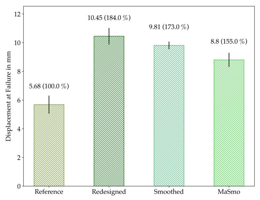
Appl. Sci. 2021, 11, 2400                                                                                                    2 of 22

                                 methods, level set methods, phase field methods, and topological derivates. Existing
                                 algorithms can be clustered into mathematical and empirical approaches. An overview
                                 can be found for instance in [17,18]. New methods are shown in [19], for instance, where
                                 neural networks are directly used in TO as an alternative to the commonly applied solid
                                 isotropic material with penalization (SIMP) approach. Today’s research in TO is often
                                 linked with additive manufacturing (AM) since its freedom of design is almost essential for
                                 fabricating topology-optimized structures [20–26]. The exploitation of lattice structures or
                                 graded porosity is of high interest in many cases [25–27]. Nevertheless, the interpretation
                                 of the optimization result and its transformation into a parametric CAD geometry is still
                                 challenging. Approaches to solving this problem can be found, for example, in [24,28,29].
                                      To enhance the manufacturability of optimized designs, manufacturing constraints
                                 are introduced [30,31]. While manufacturing constraints of casting processes have been
                                 of high interest since the early 2000s [6,29,32–34], the focus of today’s research is shifting
                                 towards AM [4,20–22,25,35–39]. The consideration of design for additive manufacturing
                                 (DfAM) aspects leads to superior solutions compared with unconstrained TO since the
                                 designs can be interpreted more efficiently and can be manufactured “as optimized” in
                                 many cases [24,39].
                                      This article presents a method to streamline the TO-based product development pro-
                                 cess from the initial design space to the ready-to-manufacture file by creating a process
                                 that is executable by “one click” and is referred to in the following as “one-click” opti-
                                 mization. The one-click optimization process, as described in Figure 1, mainly consists
                                 of TO using the topology optimization for stiffness and strength (TOSS) algorithm [40]
                                 followed by a two-step smoothing algorithm [41] for postprocessing. Furthermore, this
                                 article introduces finite sphere-based manufacturing constraints to consider DfAM
                                 aspects [42]. With these functionalities, it is possible to widely automate the conventional
                                 product development process.

      Figure 1. The visualization of the presented one-click optimization approach. The one-click tool aims to re-place and to
      widely automate the steps of topology optimization, smoothing, data exchange and redesign and finite element analysis,
      which are shown inside the green shaded area.

                                    This article investigates the performance of one-click optimized parts compared to
                                 manually redesigned parts and the initial design space. Therefore, the parts are additively
                                 manufactured and experimentally tested using a universal testing machine. The main goal
Appl. Sci. 2021, 11, 2400 3 of 22
is to show if the one-click optimized parts can be used as alternatives to the redesigned
parts, leading to faster product development for optimized lightweight structures. The
presented one-click optimization method is implemented in the TO freeware Z88Arion®
(developed by the Chair of Engineering Design and CAD, University of Bayreuth, Bayreuth,
Germany) and is available at [43].
2. Materials and Methods
The following section describes the various steps used in the one-click optimization
method in detail. In addition, it introduces the application example and explains the testing
and evaluation procedure.
2.1. Topology Optimization for Stiffness and Strength
For TO, the freeware Z88Arion® was used, which was based on density methods for
TO. While in general, the SIMP and rational approximation of material properties (RAMP)
were implemented, SIMP was used for all optimizations presented in this article. The SIMP
method thereby is given as
E(ρi ) = ρi p E0 , (1)
where E describes the adapted Young’s modulus of the material, respectively, E0 describing
the Young’s modulus for the solid material, ρ is the design variable and p the penaliza-
tion factor [17,40].
The used TOSS algorithm was developed in [40]. It is a hybrid TO algorithm, where
first a minimum compliance optimization problem is solved by using the optimality
criterion method (OC) [17]. The optimization problem for this first step can be written
as follows:
minC = minu T Ku, (2)
where C denotes the compliance, u describes the displacement vector and K the stiffness
matrix. The optimality criterion Bi after [18,40] is then given as
u T ∂ρ
∂K
u λi µ
Bi = i
= 1+ − i0 , (3)
ϑv0i ϑvi0 ϑvi
with ϑ, λ and µ as Lagrange multiplicators and v0i the volume of the initial elements. To
satisfy the optimality criteria in Equation (3), Bi has to be equal to 1 for all elements i. This
finally leads to the following iteration rule:
max 0, ρ k−α i f ρ k Bη ≤ max 0, ρk − α
i i i i
ρik+1 = ρik Bi
η η
i f max 0, ρik − α < ρik Bi < min 1, ρik + α (4)
min 1, ρk + α η
i f ρik Bi ≥ min 1, ρik + α
i
with a step length α and a damping factor η so that a decision for the new design variable
can be made with consideration of the design variable at iteration step k.
After convergence was obtained, a strength optimization was started based on em-
pirical TO approach. In this case, the soft kill option (SKO) was used, which used the
biological rule of growth to maximize the strength. This was done by achieving a homo-
geneous surface tension [18,40,44]. In this procedure, during the finite element analysis
(FEA) for each node j the equivalent stress σik−1 was computed. The equivalent stress
was then used to simulate the biological rule of growth. In contrast to mathematical TO
approaches, Young’s modulus of the elements was directly modified. This modification
can be easily done by varying the node temperatures of the finite elements. It emphasizes
here that these temperatures have no physical meaning and are only used to easily modify
Young’s modulus. This possible since Young’s modulus can be defined as a function of the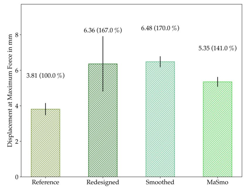
Appl. Sci. 2021, 11, 2400 4 of 22
element temperatures in every FEA software [18]. Therefore, a virtual temperature T k was
computed for each node j inside the design space:
Tjk = T̂jk + s σik−1 − σref , (5)
with:
i f T̂jk−1 > 100
100
k
T̂j = T̂jk−1 else (6)
T̂jk−1
0.1 if < 0.1
and the scaling factor s and reference stress σref , which are the user-defined inputs. The
virtual temperature is then calculated for each element i:
nl
1
Tik =
nE ∑ Tjk (7)
j= n f
where n E represents the number of nodes per element, correspondingly describes n f , the
first node which belongs to the element and nl , the last node. The Young’s modulus for
each element is then evaluated by
Emax − Emin
Ei = ( Ti − Tmin ) + Emin Ti . (8)
Tmax − Tmin
After the strength optimization converged, the final design proposal was obtained.
The conceptual procedure of the TOSS algorithm is shown in Figure 2.
Figure 2. Conceptual procedure of the topology optimization for stiffness and strength (TOSS) algorithm.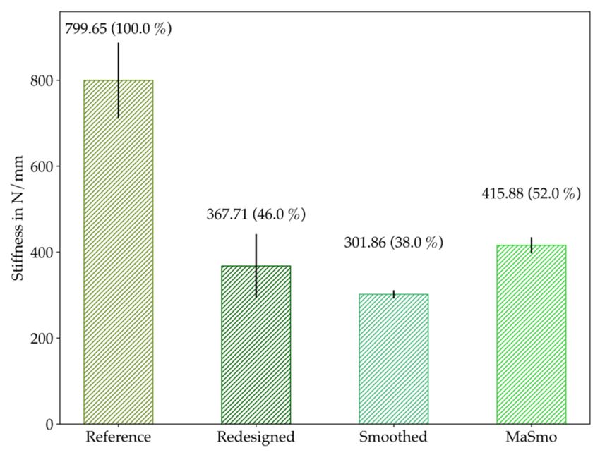
Appl. Sci. 2021, 11, 2400                                                                                                       5 of 22

                                  2.2. Finite Spheres as Manufacturing Constraints
                                       The concept of finite spheres means a useful manufacturing constraint for casting
                                  processes and AM as it describes and solves manufacturing conflicts [42]. For the im-
                                  plementation of the concept of finite spheres to the TO problem, we assumed that every
                                  element has a physically reasonable volume. Then, each element was abstracted by a
                                  sphere with an identical center of gravity and volume Vi . Therefore, the effective radius r
                                  of the sphere for element i is:             r
                                                                              3 3 Vi
                                                                        ri =         sin t                                 (9)
                                                                                4π
                                                                  π
                                  with a tolerance angle t ∈ 0, 2 . The tolerance angle is a solely technical tool which
                                  was used later to describe a manufacturing conflict. Basically, the idea is not to evaluate
                                  the elements but the finite spheres if they have manufacturing conflicts. A manufacturing
                                  conflict is defined here as two spheres with overlapping radii. In the context of casting
                                  processes, this describes an undercut. Hence, the tolerance angle can be used to specify
                                  that an overlapping only occurs, if two spheres encounter in an angle below t. Therefore,
                                  the effective radius of the spheres was adapted as shown in Figure 3.

      Figure 3. Determination of the effective radii with the tolerance angle; S denotes the center of gravity: (a) the spheres
      with unadjusted radii collide in angle t; (b) the radii are multiplied with sin t; so that (c) the spheres can pass without
      overlapping.

                                       This abstracted concept was then applied to calculate manufacturing conflicts in a
                                  given manufacturing direction s (stacking direction AM; demolding direction, casting) in
                                  combination with a manufacturing angle ω (critical printing angle AM; demolding angle,
                                  casting) as illustrated in Figure 4.
                                       Since we are generally interested in obtaining symmetric solutions, this consideration
                                  was performed in the positive and negative direction. This led to two cones for potential
                                  manufacturing conflicts as shown in Figure 5.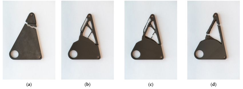
Appl. Sci. 2021, 11, 2400                                                                                                    6 of 22

                            Figure 4. Spheres with (red) and without (green) manufacturing conflict potential to the grey sphere
                            in manufacturing direction s and manufacturing angle ω.

                            Figure 5. Visualization of the conflict cones in the positive (+s) and negative (−s) direction. Conflict
                            spheres in red and conflict-free spheres in green. The conflict spheres in the positive direction are
                            stored in K+ , while the conflict spheres in negative direction are stored in K− .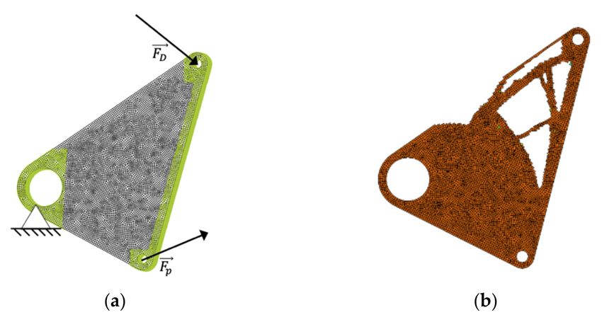
Appl. Sci. 2021, 11, 2400 7 of 22
These simplifications allowed to mathematically characterize the manufacturing con-
flicts. In this context, a casting part was manufacturable, if the geometry can be demolded
in a given angle and direction. An AM part, exemplarily a fused filament fabrication
part, could be fabricated without support structures in a given stacking direction, if the
critical printing angle was below a certain value, commonly 45 degrees. The sets Ki± of the
potential conflict elements for each element is then given by
n 2 2 o
2
Ki± = > 0 ∧ 1 − sin2 ω ||s||22 Sij 2 − s·Sij
j : ± s· Sij < ||s||2 ri + r j ± s· Sij sin ω , (10)
with the center of gravity Sij . Thereby two sets, which contain all potential positive conflict
elements, respectively, in the negative manufacturing direction, were obtained for each
element. In order to consider also previously defined passive regions, their elements were
gathered in fix sets which are defined as follows:
F0 : deactivated Elements, ρi = 0
(11)
F1 : activated Elements, ρi = 1
Hence, at the beginning of the optimization, no areas with ρi = 0 existed, the set
F0 is a priori empty. If due to the fix sets, in manufacturing direction material was fol-
lowed by a gap and then again by material, however, this gap has to be closed, so that
the manufacturing conflict can be solved. Therefore, the sets K ± are defined as fix set-
induced conflict sets, which were updated along with the algorithm as the elements
were (de-)activated:
K ± := Ui ∈ F1 Ki± \ F0 ∩ F1 ,K := K + ∪ K − . (12)
These settings were then used to remove the manufacturing conflict elements from
the optimization problem. Therefore, the part was changed stepwise in the direction of
the local mass difference towards the nearest manufacturing conflict free part. To evaluate
mass differences, the element mass mi is calculated as
mi = ρi Vi . (13)
Since real existing parts have a continuous geometry, it is obvious that this part had to
be continuous in the manufacturing direction. Therefore, it was sufficient to determine the
optimal margin of the part in the manufacturing direction. To evaluate the optimal margin,
the design variable for all elements inside of the margin was set to 1, respectively, 0 for all
elements outside of the margin. The optimal margin was then chosen, so that the deviation
between the density distribution of the optimization result and the margin was minimal.
Hence, the following equation defines the remaining loss Mi , then the considered element
is interpreted as a component of the local part surface, which is given by
Mi : = ∑ m ρ
j j i f i ∈ K ±
∧ K ±
∩ K ±
i = ∅ ; else 0
j ∈K ± ∩Ki± ∪{i }
(14)
+ ∑ (1 − ρi ) i f i ∈ K ± ∧ K ± ∩ Ki± = ∅; else 0
± ±
j ∈K ∩Ki ∪{i }
for all i ∈ K. Therefore, Mi is 0, if the element is not on the actual margin of the set K. This
definition was used to estimate the shape of the conflict-free part on the margins of set K.
This was used as an iterative decision tool, for which elements from K belong to the nearest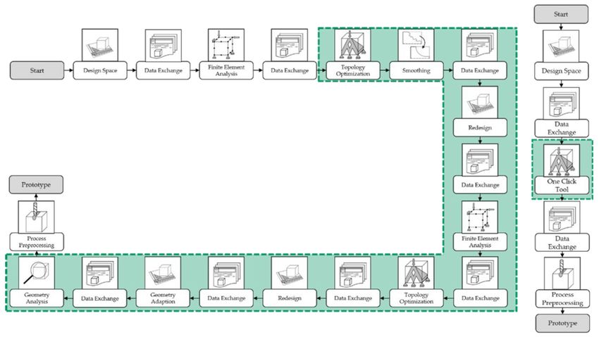
Appl. Sci. 2021, 11, 2400                                                                                                                8 of 22

                                     conflict-free part. Hence, a stepwise adaption is only reasonable for elements which are on
                                     the margin of K. The margin sets:

                                                           ∂K := i ∈ K ± : K ± ∩ Ki± = ∅ ∨ K ± ∩ Ki± = ∅

                                                                                                                            (15)

                                     with the maximizing objective function:

                                                                                   f : ∂K → R0+ , i 7→ Mi                                 (16)

                                     used to determine the next adaption of the solution geometry.
                                          The adaption was performed by the activation or deactivation of elements. More
                                     precisely, an element was activated (xi = 1) if it was inside the margin and deactivated
                                     (xi = 0) if the element was outside of the margin. It was not intended to overwrite the
                                     density distribution of the superior TO, the (de-)activation depends on the actual value
                                     of the design variable. Therefore, for symmetry reasons, the following applies to each
                                     design variable:
                                                                      a0 ( ρ i ) = 1 − a1 (1 − ρ i ),                     (17)
                                     whereby a0 describes the deactivating function and a1 describes the activation function,
                                     which is given by
                                                                                          1 − ρi
                                                                    a1 ( ρ i ) = x i +     4ρ (1− g)
                                                                                                                         (18)
                                                                                       1 + i g2

                                     where g ∈ [0, 1] is the manufacturing rate. For g = 0, the calculation of manufacturing
                                     conflicts is deactivated.
                                          This concept for considering manufacturing constraints in AM and casting processes
                                     was implemented in Z88Arion® and was applied in the following experiments. Further
                                     information on the implementation and theory of the finite sphere concept can be found
                                     in [32] and the Z88Arion® documentation on [33].

                                     2.3. Two-Step Smoothing
                                            Smoothing is a common post-processing operation which helps to make the TO result
                                     more convenient for the human eye and also allows to pass the geometry directly to the
                                     production. Therefore, it is an essential step for achieving a fully automated product
                                     development process. In this article, the implicit two-step smoothing algorithm, developed
                                     in [41] was used for the post-processing of the TO results. For the smoothing algorithm,
                                     the densities of the individual nodes j are needed. Hence, they had to be computed from
                                     the element densities of the elements which contained this particular node. These elements
                                     were further referred to as relevant elements. Hence, for each relevant element, the vectors
                                     → →            →
                                      x 1 , x 2 and x 3 from the node to its directly adjacent neighbors, as shown in Figure 6,
                                     were needed.
                                            Based on these vectors, the angle Ω, for which the element i encloses around the node
                                     j, is calculated according to [41] by
                                                                            →     →        →
                                                                             x 1 j,i , x2 j,i , x 3 j,i

                   1
               tan   Ω          =                                                                                                   .    (19)
                   2 j,i            →         →         →
                                                                 →           →
                                                                                               →      →
                                                                                                                →         →
                                    x 1 j,i   x 2 j,i   x 3 j,i + x 1 j,i   · x 2 j,i x3 + x 1 j,i · x 3 j,i x2 + x 2 j,i · x 3 j,i x1

                                          The angle Ω was then multiplied by the value of the design variable of the considered
                                     element and was normalized with the sum of all angles of the relevant elements. This
                                     procedure was repeated and summed up to obtain the final node density [41]. In the actual
                                     smoothing process, the first step was performed by a slightly modified marching cube
                                     algorithm, where the node densities were used to determine which should be part of the
                                     smoothed TO result. Consequently, in the first step, a part with a defined surface based
                                     on the node density was created by placing triangles in appropriate places to obtain the
                                     surface of the part in the Standard Tessellation Language (STL) format. The second step
                                     was based on the implicit fairing approach, which was built on Laplace smoothing and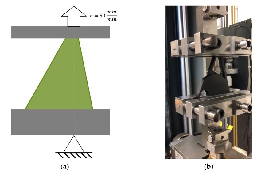
Appl. Sci. 2021, 11, 2400                                                                                          9 of 22

                            was solved using implicit integration [41]. The smoothed STL-files were then directly
                            transferred to the AM preprocessing software.

                            Figure 6. Vectors from the node j on element i to its adjacent neighbor nodes.

                            2.4. Example of Application
                                 To validate the developed “one-click” optimization process, a test-part should gen-
                            erally be suitable to manufacture with AM processes and TO. Ideally, the main objective
                            functions of the part were the minimum mass and maximum stiffness. With AM and TO
                            aspects in mind, a rocker is a well-suited example of an application for the “one-click”
                            optimization framework.
                                 Rockers are part of cars’ suspension-system and are mainly used in racecars or ex-
                            pensive super-sportscars like the Lamborghini Aventador. Two of its essential aspects
                            are stiffness and mass. Stiffness is of importance to prevent unnecessary play in the
                            suspension-system, which can result in negative balance and drivability [45].
                                 In general, car suspensions link the upright (or knuckle) assembly with the car’s
                            body [45]. The upright assembly’s main parts are the wheel bearings, wheel hubs, brake
                            calipers, and the suspension’s fastening points; these are attached to the car’s body by
                            different types of links. The complexity and type of the links often vary with car pricing or
                            comfort aspects [45].
                                 Most modern production road cars use directly actuated shock absorbers and coil
                            springs either by a MacPherson strut or a multilink suspension [45,46]. Two typically used
                            systems are shown in Figure 7. Directly actuated refers to a one-to-one motion ratio of the
                            coupled suspension-link and the spring-damper unit.
                                 Nevertheless, the double-wishbone suspension with a rocker as part of the pushrod
                            activated spring-damper unit, displayed in Figure 8, is used in some races—in super-
                            sportscars. These low part volumes make the rocker potentially suitable to be replaced by
                            optimized AM parts in the future, and therefore, are an appropriate example of application.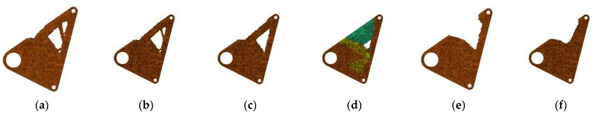
Appl. Sci. 2021, 11, 2400                                                                                               10 of 22

                            Figure 7. Typical front suspension systems: (a) McPherson; and (b) double wishbone.

                                     Figure 8. Double wishbone suspension with pushrod (red), rocker (green) and spring-damper
                                     unit (grey).

                                          In the double-wishbone suspension, the wheel travels upwards, the pushrod moves
                                     longitudinal to its axis, and rotates the rocker around a fixed pivot point, which results
                                     in the spring-damper unit’s compression. This causes two loads acting on the rocker, the
                                                                             →
                                     compression force from the pushrod FP and the difference between the compression force
                                                                              →
                                     from the spring and the damper unit FD .
Appl. Sci. 2021, 11, 2400 11 of 22
Based on its assembly situation and working principle, the following initial design
space in Figure 9 with its related forces was considered for the rocker optimization task.
The particular values of the force components are listed in Table 1.
Figure 9. Initial design space of the rocker chosen for TO and AM with its related forces.
Table 1. Force components for the chosen topology optimization (TO) problem. The values are based
on the measurements of a formula student racecar [47].
Force Component Value in N
→
FD,x 455
→
FD,y −750
→
Fp,x 2960
→
Fp,y 2770
2.5. Testing and Validation
The rocker in Figure 9 was used for the testing and validation of the method. Therefore,
the initial design space was the reference model, and three various TO configurations were
selected. This led to four configurations that were printed in total. The initial design space
of the rocker was elected as the reference configuration (Reference). The TO configurations
were as follows: an optimized part without the consideration of manufacturing conflicts
and manually redesigned (redesigned); an optimized part without consideration of manu-
facturing conflicts and smoothed (Smoothed); and an optimized part with the consideration
of manufacturing conflicts and smoothed (MaSmo). All TO runs had a volume constraint
of 75% of the initial design space.Appl. Sci. 2021, 11, 2400 12 of 22
All parts were manufactured using the Markforged MarkTwo (Markforged Inc.,
Boston, MA, USA) and Onyx [48] as material for all specimens. For each configura-
tion, ten specimens were printed. The parts were printed with a triangular infill of 37%,
4 roof-, 4 floor- and 2 wall-layers, which were the default settings in the used preprocessing
software Eiger (Markforged Inc., Boston, MA, USA). For the MaSmo Configuration, the
stacking direction was in alignment with the manufacturing direction (z axis in Figure 9).
The testing was done on a universal testing machine, where the parts were clamped
as shown in Figure 10 and uniaxial stressed. The traverse speed during all experiments ias
50 mm per minute.
Figure 10. Experimental set-up: (a) sketch; and (b) actual experimental set-up.
The chosen experimental set-up deviates from the most relevant loads shown in
Figure 9. This is because parts were optimized according to the most common loads and
boundary conditions in use, but the part also had to withstand several other types of load
settings that were not considered in TO. Therefore, the chosen boundary conditions and
loading of this set-up reflect a critical load-case when the wheel was blocked, which is one
example of an additional load case to be considered during the part’s design.
For the evaluation, the manufacturability of the design proposals, the printing time,
and the parts’ actual target volume were discussed. In evaluating the mechanical perfor-
mance, the parts were investigated regarding their maximum forces, displacements, and
stiffness at maximum stress.
3. Results
The TO set up according to the loads in 2.4. and the TO result without the consideration
of manufacturing conflicts are shown in Figure 11.Appl. Sci. 2021, 11, 2400 13 of 22
Figure 11. Tested configurations of the rocker: (a) TO setup, the green areas are non-design spaces;
and (b) TO result without the consideration of the manufacturing conflicts.
The derived post-processed TO design proposals are shown in Figure 12, the configu-
rations smoothed and MaSmo are smoothed using 50 smoothing iterations. This number
is empirically obtained from extensive studies with Z88Arion and has been proven to
provide error-free STL-files in most cases. The settings chosen for the consideration of the
manufacturing conflicts and are presented in detail in the next section. The redesigned
configuration aims to stay as close to the original TO result as possible. The MaSmo
configuration differs significantly from the other ones.
Figure 12. Tested configurations of the rocker. (a) reference; (b) redesigned; (c) smoothed; (d) MaSmo.
As listed in Table 2, a target volume for all TO runs is 75%; nevertheless, the post-
processed parts’ real volume differs from this target. Since the deviations are small in all
cases, it is reasonable that the geometry adaption of the MaSmo configuration according to
the least mass loss is reasonable.
It is further important to mention that MaSmo shows the best convergence behavior
at the chosen TO settings.Appl. Sci. 2021, 11, 2400 14 of 22
Table 2. Overview of the TO settings of all configurations. Since reference is the initial design space, no TO is performed for
this configuration. All volumes are referenced on the volume of the reference configuration.
Configuration Algorithm Manufacturing Constraints Target Volume Real Volume Iterations
Reference – – 100% 100% –
Redesigned TOSS no 75% 77.2% 100
Smoothed TOSS no 75% 74.6% 100
MaSmo TOSS Yes 75% 75.6% 41
3.1. Manufacturability of Design Proposals
In this article, the previously described formulation of manufacturing conflicts im-
proves the obtained design proposals’ direct manufacturability. The manufacturing rate
controls the strictness of the manufacturing conflicts. As avoiding support at all costs is
not always a goal-orientated approach, the manufacturing conflict rate is modified in the
range of 0.5–1.0 to determine the appropriate manufacturing rate for the given application
example. The results are given in Figure 13.
Figure 13. TO results for various manufacturing rates g. All elements whose design variable is greater than 0.1 are displayed.
Additionally, the number of iterations until convergence is noted (a) g = 0.5 iterations: 87; (b) g = 0.6, iterations: 41;
(c) g = 0.7 iterations = 41; (d) g = 0.8 iterations: 99; (e) g = 0.9 iterations: 99; and (f) g = 1.0 iterations: 100.
Based on the results in Figure 13, a manufacturing rate of g = 0.7 is chosen for the
MaSmo configuration, as it is a good compromise between the original TO result and
improved manufacturability. Furthermore, the influence of the manufacturing angle ω is
shown in Figure 14.
Figure 14. TO results for various manufacturing angles ω at the manufacturing rate g = 0.7, all elements whose design
variable is greater than 0.1 are displayed. Additionally, the number of iterations until convergence is noted. (a) ω = 15 deg,
iterations: 76; (b) ω = 45 deg, iterations: 41 (c) ω = 75 deg, iterations: 100.
These results show that the manufacturing angle also heavily influences the conver-
gence behavior of the TO. Moreover, the precise effect of the manufacturing angle on the TO
result shows that the method works. For selecting the appropriate manufacturing angle, aAppl. Sci. 2021, 11, 2400 15 of 22
common practice is followed by choosing 45 deg. To shortly summarize the manufacturing
conflict settings, an overview is given in Table 3.
Table 3. Overview of the manufacturing conflict settings chosen for MaSmo.
Feature Value
Manufacturing direction z axis
Manufacturing rate 0.7
Manufacturing angle 45 deg.
Subsequently, all four configurations are additively manufactured. The resulting print-
ing times, actual plastic volumes deposited in total, and support volumes are compared in
Table 4.
Table 4. Manufacturing data overview. The plastic volume is the actual volume used in production and is referenced on the
reference plastic volume. The support volume of redesigned is used as a reference for the comparison of the needed support
volume. The support volume ratio is defined by the ratio of the used support structures to the plastic volume.
Configuration Print Time Plastic Volume Support Volume Support Volume Ratio
Reference 100% 100% – –
Redesigned 103.2% 92.0% 100% 0.76%
Smoothed 104.3% 90.0% 131.6% 1.03%
MaSmo 95.3% 88.9% 52.6% 0.42%
It is important to note that there is a significant change in the relative values between
the plastic volume and the real volume after TO. MaSmo leads to shorter print time,
and additionally, the needed support volume can be reduced by 47.4%. In addition, it is
important to emphasize here that for redesigned, the support volume takes 0.76% of the
total plastic volume.
3.2. Experimental Testing
The printed and experimentally tested specimens are shown in Figure 15.
Figure 15. Printed and tested specimens: (a) reference; (b) redesigned; (c) smoothed; and (d) MaSmo.
The force–displacement plots are illustrated in Figure 16. The measured data’s qualita-
tive mean curves are obtained by using a Gaussian process regression (gpr) model trained
with the experimental data. Therefore, a radial basis function kernel with an added white
kernel to handle the noise is used [49].Appl. Sci. 2021, 11, 2400 16 of 22
Figure 16. Force–displacement plots for all configurations. The grey shaded lines are the experimental
data, the green lines are predicted with the trained Gaussian process regression (gpr) model.
From the presented data, it is evident that the MaSmo configuration was the least noisy,
leading to a good reproducibility of the “one-click” optimized part. The approximated
curves of all configurations are compared in Figure 17.
Figure 17. Comparison of the approximated force–displacement behavior of all configurations. The
red dotted line indicates the level 75% of the reference’s maximum force.Appl. Sci. 2021, 11, 2400 17 of 22
From this comparison, it can be evaluated that the maximum forces of redesigned
and MaSmo are quite identical while smoothed performed significantly lower; this can be
confirmed by evaluating the maximum forces in Figure 18.
Figure 18. Comparison of the maximum forces. The mean values are plotted together with the
standard deviation. The difference from the reference is written in brackets in percent.
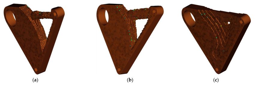
The displacements are evaluated in detail in Figures 19 and 20.
Figure 19. Comparison of the displacement at failure. The mean values are plotted together with the
standard deviation. The difference from the reference is written in brackets in percent.Appl. Sci. 2021, 11, 2400 18 of 22
Figure 20. Comparison of the displacement at maximum force. The mean values are plotted together
with the standard deviation. The difference from the reference is written in brackets in percent.
In general, it can be observed that the displacements at failure and maximum force
are on the same level for redesigned and smoothed, whereas the values for MaSmo are the
lowest for the TO-configurations. The high standard deviation of redesigned is also to be
emphasized here.
Since in particular cases TO maximizes the stiffness, the stiffness at maximum force is
evaluated for all configurations in Figure 21.
Figure 21. Comparison of the stiffness at maximum force. The mean values are plotted together with
the standard deviation. The difference from the reference is written in brackets in percent.Appl. Sci. 2021, 11, 2400 19 of 22
In this context, MaSmo clearly outperforms smoothed and slightly outperforms re-
designed. Additionally, the standard deviation for MaSmo is significantly lower than for
reference and redesigned.
4. Discussion
The objective of this article was to show the competitiveness of “one-click” devel-
oped TO prototypes in comparison to more conventional approaches. Therefore, finite
spheres are used to add manufacturing constraints during the optimization. Since using
an absolute strictness in preventing manufacturing conflicts may not always be expedient,
it is reasonable to control the manufacturing constraints within certain limits. The final
chosen settings are based on numerical convergence behavior and also on the common
practice in AM. Hence, it is assumed that the settings in Table 3 show a good mixture of
numerical convergence behavior and increased manufacturability of the design proposal.
It is important to emphasize here that while in AM support structures can be tolerated,
undercuts in casting processes are non-tolerable. It is further shown in Table 4 that the
chosen settings lead to the configuration with the least printing time and also requires the
least material in production.
Nevertheless, the trade-off of the relative volumes between the final STL volume and
the needed plastic volume in production is important to mention. This trade-off is an effect
of using shelled parts, as it is standard in fused filament fabrication. Hence, methods as
presented in [20], which consider shelled AM parts directly for TO, must be the subject
of future work. Summing up, in terms of manufacturability, the one-click optimization
method leads to design proposals (MaSmo), which are better suited for AM than the
other configurations.
The used test setup in Figure 10 is an abstracted critical load case for the presented
application example. Due to this fact, the chosen setup is qualified to evaluate the various
configurations’ mechanical performances. Regarding the testing results in Figure 16, it is
important to stress that the MaSmo configuration was the least noisy. In addition, MaSmo
and redesigned are comparable and both better than smoothed in terms of maximal forces.
Since the used TO approach is a hybrid optimization for stiffness and strength, it is assumed
that TO configurations can bear about 75% of the reference’s maximum force, which is met
quite accurately by MaSmo and Redesigned with 74% of the maximum force. In terms of
stiffness, compared in Figure 21, the “one-click” optimized MaSmo configuration shows
the best result, which corresponds to 52% of reference’s stiffness.
These results assume that the presented “one-click” optimization approach is compet-
itive to conventional TO with redesign of the design proposals, as it achieves comparable
results for the maximum force and slightly better results for the part stiffness. Therefore,
the developed approach allows the manufacture of topologically optimized prototypes in
AM directly with a minimum of needed user inputs and is a nearly fully automated design
process for the rapid production of prototypes. Since only solid parts are considered, it is
an essential objective of future work to integrate graded porosity in combination with unit
cells or triple periodic minimalized surface structures as shown in [25] into the “one-click”
optimization approach in order to be more sophisticated towards AM. In addition, an
improvement in the post-processing of the TO results using techniques like support vector
regression [28] can further enhance the framework’s usability.
5. Conclusions
In this article, the one-click optimization approach was shown under the direct man-
ufacturing of optimized prototypes in additive manufacturing. The approach consists
of a hybrid topology optimization algorithm for stiffness and strength, finite spheres for
considering manufacturing constraints, and a two-step smoothing algorithm for post-
processing. The approach was exemplarily shown on a rocker and experimentally tested
and compared with conventional topology optimization and redesigning. The results
state that the one-click optimized parts show comparable or slightly better mechanicalAppl. Sci. 2021, 11, 2400 20 of 22
testing performance while clearly showing superior performance in convergence behavior
and manufacturing. Therefore, the one-click optimization approach can be successfully
applied to the nearly fully automated direct manufacturing of optimized prototypes using
additive manufacturing.
Author Contributions: Conceptualization, T.R.; methodology, T.R.; software, M.Z., T.S. and T.R.;
validation, T.R., R.H. and M.Z.; formal analysis, T.R. and T.S.; investigation, T.R. and R.H.; resources,
T.R. and T.S.; data curation, T.R.; writing—original draft preparation, T.R. and R.H.; writing—review
and editing, C.K. and M.Z.; visualization, T.R., R.H. and C.K.; supervision, C.K., B.A.-L. and F.R.;
project administration, B.A.-L. and F.R.; funding acquisition, B.A.-L. and F.R. All authors have read
and agreed to the published version of the manuscript.
Funding: This research was funded by the European Regional Development Fund (EFRE) and the
APC was funded by the German Research Foundation (DFG) and the University of Bayreuth in the
funding program Open Access Publishing.
Institutional Review Board Statement: Not applicable.
Informed Consent Statement: Not applicable.
Data Availability Statement: The software and all data presented in this study are available at
www.z88.de (accessed on 10 February 2021).
Conflicts of Interest: The authors declare no conflict of interest.
References
1. Glamsch, J.; Deese, K.; Rieg, F. Methods for Increased Efficiency of FEM-Based Topology Optimization. Int. J. Simul. Model. 2019,
18, 453–463. [CrossRef]
2. Billenstein, D.; Dinkel, C.; Rieg, F. Automated Topological Clustering of Design Proposals in Structural Optimisation. Int. J. Simul.
Model. 2018, 17, 657–666. [CrossRef]
3. Berrocal, L.; Fernández, R.; González, S.; Periñán, A.; Tudela, S.; Vilanova, J.; Rubio, L.; Márquez, J.M.M.; Guerrero, J.; Lasagni, F.
Topology optimization and additive manufacturing for aerospace components. Prog. Addit. Manuf. 2018, 4, 83–95. [CrossRef]
4. Guo, X.; Zhou, J.; Zhang, W.; Du, Z.; Liu, C.; Liu, Y. Self-supporting structure design in additive manufacturing through explicit
topology optimization. Comput. Methods Appl. Mech. Eng. 2017, 323, 27–63. [CrossRef]
5. Zhan, J.; Luo, Y. Robust topology optimization of hinge-free compliant mechanisms with material uncertainties based on a
non-probabilistic field model. Front. Mech. Eng. 2019, 14, 201–212. [CrossRef]
6. Wang, Y.; Kang, Z. Structural shape and topology optimization of cast parts using level set method. Int. J. Numer. Methods Eng.
2017, 111, 1252–1273. [CrossRef]
7. Tsavdaridis, K.D.; Kingman, J.J.; Toropov, V.V. Application of structural topology optimisation to perforated steel beams. Comput.
Struct. 2015, 158, 108–123. [CrossRef]
8. Lagaros, N.D.; Papadrakakis, M.; Kokossalakis, G. Structural optimization using evolutionary algorithms. Comput. Struct. 2002,
80, 571–589. [CrossRef]
9. Sigmund, O. On the Design of Compliant Mechanisms Using Topology Optimization*. Mech. Struct. Mach. 1997, 25, 493–524.
[CrossRef]
10. Larsen, U.D.; Signund, O.; Bouwsta, S. Design and fabrication of compliant micromechanisms and structures with negative
Poisson’s ratio. J. Microelectromech. Syst. 1997, 6, 99–106. [CrossRef]
11. Srivastava, S.; Salunkhe, S.; Pande, S.; Kapadiya, B. Topology optimization of steering knuckle structure. Int. J. Simul. Multidiscip.
Des. Optim. 2020, 11, 4. [CrossRef]
12. Ismail, A.Y.; Na, G.; Koo, B. Topology and Response Surface Optimization of a Bicycle Crank Arm with Multiple Load Cases.
Appl. Sci. 2020, 10, 2201. [CrossRef]
13. Shi, G.; Guan, C.; Quan, D.; Wu, D.; Tang, L.; Gao, T. An aerospace bracket designed by thermo-elastic topology optimization and
manufactured by additive manufacturing. Chin. J. Aeronaut. 2020, 33, 1252–1259. [CrossRef]
14. Calabrese, M.; Primo, T.; Del Prete, A. Optimization of Machining Fixture for Aeronautical Thin-walled Components. Procedia
CIRP 2017, 60, 32–37. [CrossRef]
15. Klippstein, H.; Hassanin, H.; Sanchez, A.D.D.C.; Zweiri, Y.; Seneviratne, L. Additive Manufacturing of Porous Structures for
Unmanned Aerial Vehicles Applications. Adv. Eng. Mater. 2018, 20, 1800290. [CrossRef]
16. TopOpt Software and Apps. Available online: https://www.topopt.mek.dtu.dk/apps-and-software (accessed on 1 March 2021).
17. Sigmund, O.; Maute, K. Topology optimization approaches. Struct. Multidisc. Optim. 2013, 48, 1031–1055. [CrossRef]
18. Harzheim, L. Strukturoptimierung Grundlagen und Anwendungen, 3rd ed.; Europa-Lehrmittel: Haan-Gruiten, Germany, 2019.
19. Chandrasekhar, A.; Suresh, K. TOuNN: Topology Optimization using Neural Networks. Struct. Multidiscip. Optim. 2020, 1–15.
[CrossRef]Appl. Sci. 2021, 11, 2400 21 of 22
20. Clausen, A.; Andreassen, E.; Sigmund, O. Topology optimization of 3D shell structures with porous infill. Acta Mech. Sin. 2017,
33, 778–791. [CrossRef]
21. Dapogny, C.; Estevez, R.; Faure, A.; Michailidis, G. Shape and topology optimization considering anisotropic features induced by
additive manufacturing processes. Comput. Methods Appl. Mech. Eng. 2019, 344, 626–665. [CrossRef]
22. Liu, S.; Li, Q.; Liu, J.; Chen, W.; Zhang, Y. A Realization Method for Transforming a Topology Optimization Design into Additive
Manufacturing Structures. Engineering 2018, 4, 277–285. [CrossRef]
23. Meng, L.; Zhang, W.; Quan, D.; Shi, G.; Tang, L.; Hou, Y.; Breitkopf, P.; Zhu, J.; Gao, T. From Topology Optimization Design to
Additive Manufacturing: Today’s Success and Tomorrow’s Roadmap. Arch. Comput. Methods Eng. 2020, 27, 805–830. [CrossRef]
24. Plocher, J.; Panesar, A. Review on design and structural optimisation in additive manufacturing: Towards next-generation
lightweight structures. Mater. Des. 2019, 183, 108164. [CrossRef]
25. Strömberg, N. Optimal grading of TPMS-based lattice structures with transversely isotropic elastic bulk properties. Eng. Optim.
2020, 1–13. [CrossRef]
26. Thompson, M.K.; Moroni, G.; Vaneker, T.; Fadel, G.; Campbell, R.I.; Gibson, I.; Bernard, A.; Schulz, J.; Graf, P.; Ahuja, B.; et al.
Design for Additive Manufacturing: Trends, opportunities, considerations, and constraints. CIRP Ann. 2016, 65, 737–760.
[CrossRef]
27. Schmidt, M.-P.; Pedersen, C.B.W.; Gout, C. On structural topology optimization using graded porosity control. Struct. Multidiscip.
Optim. 2019, 60, 1437–1453. [CrossRef]
28. Strömberg, N. Automatic Postprocessing of Topology Optimization Solutions by Using Support Vector Machines. In Proceedings
of the ASME 2018 International Design Engineering Technical Conferences & Computers and Information in Engineering
Conference IDETC/CIE 2018, Quebec City, QC, Canada, 26–29 August 2018. [CrossRef]
29. Harzheim, L.; Graf, G. A review of optimization of cast parts using topology optimization. Struct. Multidiscip. Optim. 2005, 30,
491–497. [CrossRef]
30. Frisch, M.; Dörnhöfer, A.; Nützel, F.; Rieg, F. Fertigungsrestriktionen in der Topologieoptimierung. In Integrierte Produktentwicklung
für Einen Globalen Markt, Proceedings of the 9. Gemeinsames Kolloquium Konstruktionstechnik, Aachen, Germany, 6–7 October 2011;
Brökel, K., Grote, K.-H., Rieg, F., Stelzer, R., Eds.; Shaker: Aachen, Germany, 2011.
31. Vatanabe, S.L.; Lippi, T.N.; De Lima, C.R.; Paulino, G.H.; Silva, E.C. Topology optimization with manufacturing constraints: A
unified projection-based approach. Adv. Eng. Softw. 2016, 100, 97–112. [CrossRef]
32. Harzheim, L.; Graf, G. A review of optimization of cast parts using topology optimization II–Topology optimization with
manufacturing constraints. Struct. Multidiscip. Optim. 2005, 31, 388–399. [CrossRef]
33. Franke, T.; Fiebig, S.; Bartz, R.; Vietor, T.; Hage, J.; Hofe, A.V. Adaptive Topology and Shape Optimization with Integrated
Casting Simulation. In EngOpt 2018 Proceedings of the 6th International Conference on Engineering Optimization, 2018; Rodrigues,
H.C., Herskovits, J., Mota Soares, C.M., Araujo, A.L., Guedes, J.M., Folgado, J.O., Moleiro, F., Madeira, J.F.A., Eds.; Springer
International Publishing: Cham, Switzerland, 2018. [CrossRef]
34. Franke, T.; Fiebig, S.; Paul, K.; Vietor, T.; Sellschopp, J. Topology Optimization with Integrated Casting Simulation and Parallel
Manufacturing Process Improvement. In Advances in Structural and Multidisciplinary Optimization, Proceedings of the World Congress
of Structural and Multidisciplinary Optimisation, Braunschweig, Germany, 5–9 June 2017; Schumacher, A., Vietor, T., Fiebig, S.,
Bletzinger, K.U., Maute, K., Eds.; Springer International Publishing: Cham, Switerland, 2018. [CrossRef]
35. Mirzendehdel, A.M.; Suresh, K. Support structure constrained topology optimization for additive manufacturing. Comput. Des.
2016, 81, 1–13. [CrossRef]
36. Gaynor, A.T.; Guest, J.K. Topology optimization considering overhang constraints: Eliminating sacrificial support material in
additive manufacturing through design. Struct. Multidiscip. Optim. 2016, 54, 1157–1172. [CrossRef]
37. Kandemir, V.; Dogan, O.; Yaman, U. Topology optimization of 2.5D parts using the SIMP method with a variable thickness
approach. In Proceedings of the 28th International Conference on Flexible Automation and Intelligent Manufacturing (FAIM2018),
Columbus, OH, USA, 11–14 June 2018. Procedia Manufacturing. [CrossRef]
38. Leary, M.; Merli, L.; Torti, F.; Mazur, M.; Brandt, M. Optimal topology for additive manufacture: A method for enabling additive
manufacture of support-free optimal structures. Mater. Des. 2014, 63, 678–690. [CrossRef]
39. Saadlaoui, Y.; Milan, J.-L.; Rossi, J.-M.; Chabrand, P. Topology optimization and additive manufacturing: Comparison of
conception methods using industrial codes. J. Manuf. Syst. 2017, 43, 178–186. [CrossRef]
40. Frisch, M. Entwicklung eines Hybridalgorithmus zur Steifigkeits- und Spannungsoptimierten Auslegung von Konstruktionsele-
menten. Ph.D. Thesis, Univeristy of Bayreuth, Bayreuth, Germany, 2015.
41. Deese, K.; Geilen, M.; Rieg, F. A Two-Step Smoothing Algorithm for an Automated Product Development Process. Int. J. Simul.
Model. 2018, 17, 308–317. [CrossRef]
42. Rosnitschek, T.; Siegel, T.; Linke, D.; Mailänder, P.; Kamp, D.; Rieg, F. Optimizing material exploitation in the direct additive
manufacturing of topology-optimized structures. In Nachhaltige Produktentwicklung, Proceedings of the 18. Gemeinsames Kolloquium
Konstruktionstechnik, Duisburg, Germany, 1–2 October 2020; Corves, B., Gericke, K., Grote, K.-H., Lohrengel, A., Löwer, M.,
Nagarajah, A., Rieg, F., Scharr, G., Stelzer, R., Eds.; University of Duisburg-Essen: Duisburg, Germany, 2020. [CrossRef]
43. Z88. Available online: https://z88.de (accessed on 10 February 2021).
44. Baumgartner, A.; Harzheim, L.; Mattheck, C. SKO (soft kill option): The biological way to find an optimum structure topology.
Int. J. Fatigue 1992, 14, 387–393. [CrossRef]Appl. Sci. 2021, 11, 2400 22 of 22
45. Ersoy, M.; Gies, S. Fahrwerkhandbuch; Springer International Publishing: Berlin/Heidelberg, Germany, 2017.
46. Trzesniowski, M. (Ed.) Fahrwerk. In Handbuch Rennwagentechnik, 2nd ed.; Springer-Vieweg: Wiesbaden, Germany, 2019; Volume 4.
47. Elefant Racing Bayreuth. Available online: https://elefantracing.de (accessed on 26 February 2021).
48. Markforged Onyx Material Data. Available online: https://markforged.com/materials/plastics/onyx (accessed on 10 Febru-
ary 2021).
49. Pedregosa, F.; Varoquaux, G.; Gramfort, A.; Michel, V.; Thirion, B.; Grisel, O.; Blondel, M.; Prettenhofer, P.; Weiss, R.; Du-bourg,
V.; et al. Scikit-learn: Machine Learning in Python. JMLR 2011, 85, 2825–2830.You can also read