Real-Time Production and Logistics Self-Adaption Scheduling Based on Information Entropy Theory - MDPI
←
→
Page content transcription
If your browser does not render page correctly, please read the page content below
sensors
Article
Real-Time Production and Logistics Self-Adaption
Scheduling Based on Information Entropy Theory
Wenchao Yang 1 , Wenfeng Li 1, *, Yulian Cao 2 , Yun Luo 1 and Lijun He 1
 1    School of Logistics Engineering, Wuhan University of Technology, Wuhan 430063, China;
      yangwc6532@gmail.com (W.Y.); yunluo@whut.edu.cn (Y.L.); helj@whut.edu.cn (L.H.)
 2    School of Aviation, University of New South Wales, Sydney, NSW 2052, Australia; yalianjingren@126.com
 *    Correspondence: liwf@whut.edu.cn

 Received: 29 June 2020; Accepted: 6 August 2020; Published: 12 August 2020

 Abstract: In recent years, the individualized demand of customers brings small batches and
 diversification of orders towards enterprises. The application of enabling technologies in the factory,
 such as the industrial Internet of things (IIoT) and cloud manufacturing (CMfg), enhances the ability
 of customer requirement automatic elicitation and the manufacturing process control. The job shop
 scheduling problem with a random job arrival time dramatically increases the difficulty in process
 management. Thus, how to collaboratively schedule the production and logistics resources in the
 shop floor is very challenging, and it has a fundamental and practical significance of achieving
 the competitiveness for an enterprise. To address this issue, the real-time model of production
 and logistics resources is built firstly. Then, the task entropy model is built based on the task
 information. Finally, the real-time self-adaption collaboration of production and logistics resources is
 realized. The proposed algorithm is carried out based on a practical case to evaluate its effectiveness.
 Experimental results show that our proposed algorithm outperforms three existing algorithms.

 Keywords: industrial internet of things; random job arrival time; information entropy theory;
 self-adaption; real-time scheduling

1. Introduction
     With the growing demand for product customization, the characteristic of orders is developing
towards diversification and small batch. Usually, the manufacturers’ goal is to minimize the completion
time and energy consumption. The factory arranges the manufacturing task according to its own goal,
which rarely considers customers’ requirements [1]. The scheduling problem with random orders has
been becoming increasingly important for smart manufacturing. Traditionally, the manufacturing
factory focuses on reducing production cost [2]. However, the goal of a smart factory involves not only
minimizing manufacturing cost, but also maximizing customer satisfaction.
     In addition, the manufacturers’ delivery delay will lead to reducing customer satisfaction and
increasing costs. Under the cloud manufacturing (CMfg) mode, each customer wants to receive
the required products from a smart factory within an expected date [3]. The manufacturers shall
meet the customer’s delivery time while considering their own production capacity limitations.
Traditional scheduling assumes that information on production resources and tasks is fully known.
This assumption is not applicable in a customized environment because customer orders will arrive
dynamically [4]. In the intelligent plant, the instantaneity demand of customers dramatically increases
the difficulty of job-shop scheduling problem (JSP), i.e., random job arrival increases the complexity of
scheduling problems [5].
     In a new manufacturing environment, such as the Internet of things and CMfg, tasks of smart
shop floor (SSF) are ordered by a cloud platform, even by customers directly [6]. When the production

Sensors 2020, 20, 4507; doi:10.3390/s20164507                                   www.mdpi.com/journal/sensors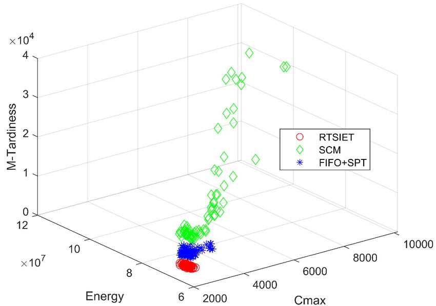
Sensors 2020, 20, 4507                                                                               2 of 17

and logistics resources are confronted with orders with a random arrival and different due date,
the traditional scheduling methods will be difficult to cope with such a new manufacturing scenario.
In the smart workshop, the coordination of production and logistics resources, as well as the random
arrival time of orders and different due dates, should be considered. Multi-resource collaboration and
resources matching optimization are vital problems that need to be solved by the smart manufacturing
system in a dynamic environment based on real-time serviceability.
      Production and logistics\manufacturing resources (PLRs\MRs) collaborative scheduling is the
basis for improving production efficiency and resolving the problem of insufficient production resources
caused by the diversified needs of customers. However, there is little guidance about how production
and logistics resources collaboration allocation affects the production decision of the remanufacturing
system, especially in the real-time manufacturing system. In reality, production and processing are main
stages that consume resources and energy, as well as the critical nodes with the most significant potential
for intelligence. Hence, this phenomenon raises some questions. How should manufacture enterprises
manage heterogeneous production and logistics resources to realize intelligence in manufacturing?
Under the uncertain environment, how should the manufacturing system dynamically allocate
real-time tasks?
      This paper proposes a production and logistics real-time adaptive scheduling method based on
information entropy to solve the above problems. The real-time scheduling method includes three
parts. (1) It builds a real-time state model of production and logistics resources for dynamic production
tasks based on real-time data of SSF; (2) it builds a standard entropy model of real-time tasks according
to the execution status and delivery time of customized orders; (3) based on the standard entropy
model of tasks and the real-time state model of resources, a real-time scheduling algorithm based on the
information entropy theory (RTSIET) is constructed for improving the efficiency of producer services.
      The main contributions of this study are summarized as follows:

1.    The RTSIET strategy based on adaptive coordination of smart resources can effectively deal with
      tasks with time constraints. It includes features that are rarely mentioned before, such as the
      allocate service resources according to due date.
2.    The adaptive scheduling strategy reduces production time, energy consumption, and delays
      through the optimization of feasible services. In addition, compared with traditional scheduling
      strategies, the RTSIET strategy developed in this paper can improve coordination ability among
      PLRs and enhance the stability of real-time scheduling.

     The remaining of this paper is organized as follows. Section 2 gives a literature review. Section 3
describes the problem of real-time manufacturing resources allocation (RTMRA) with a scenario
description. Section 4 presents the conceptual model and the information model. Section 5 describes
the overall solution and fundamental algorithms for RTMRA. Based on a practical case, Section 6
represents and analyzes the research results of this paper. Section 7 highlights the conclusions and
provides future works.

2. Related Work
     The flexible job-shop scheduling problem (FJSP) is an outgrowth of the classic job shop scheduling
problem (JSP), which has multi-function machines [7]. During the past three decades, there has been
extensive development of efficient techniques for solving the FJSP in the traditional manufacturing
industry [8]. Evolutionary algorithms (EAs), such as particle swarm optimization (PSO) algorithm [9]
and fireworks algorithm (FWA) [10], show advantages in solving optimization problems. Some popular
EAs, such as PSO, FWA, genetic algorithm, etc., which are applied to traditional FJSP, have achieved
excellent results [11,12]. Although researchers have tackled the JSP with various brilliant approaches,
there are limitations when dealing with practical implementation under an ever-changing modern
environment where a real-time scheduling decision is required due to unpredictable systems
disturbances at any second [13].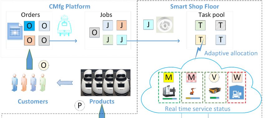
Sensors 2020, 20, 4507                                                                             3 of 17

      The production of a smart flexible job shop (SFJS) with a distinct due window of multi-customer
increases the difficulty of job shop scheduling. Hence, traditional flexible job shop scheduling
methods are difficult to adapt to new conditions. As a kind of data-driven knowledge model,
the manufacturing resource allocation (MRA) model is of critical importance in the manufacturing
industry, which determines the efficiency and flexibility of a shop floor and its production system [14].
Smart manufacturing resources, e.g., machines, vehicles, and work-in-progress (WIP), in SFJS have
self-configuration, self-learning, and self-decision intelligence [15,16].
      In the environment of industrial Internet of things (IIoT), real-time manufacturing resources
allocation (RTMRA) can be further developed to make full use of the interconnection among
manufacturing resources to achieve intelligent cooperation [17]. Therefore, it is timely and crucial to
consider adaptive scheduling and control (i.e., RTMRA) for dynamic manufacturing environments
as crucial research issues in smart production management [18]. The timely feedback shop floor
information during the manufacturing execution stage leads to a significant improvement in achieving
real-time production scheduling [19]. Luo et al. [20,21] proposed to integrate wired and wireless
networks by also taking advantage of the automated guided vehicle (AGV) in smart factories,
which increases data delivery efficiency. Zhang et al. [22] presented an overall architecture of
multi-agent-based real-time production scheduling to close the loop of production planning and
control. Shiue et al. [23] proposed a reinforcement learning (RL)-based RTS using the multiple
dispatching rules mechanism to respond to changes in the shop floor environment. Ding et al. [15]
trained a hidden Markov model (HMM)-based knowledge model from the historical data for smart
manufacturing resources (SMRs) to allocate themselves autonomously for manufacturing tasks. Zhang
and Wang [24,25] proposed an allocation strategy based on the game optimization model for real-time
tasks. Both production resources (PRs) and logistics resources (LRs) in SSF are created as an inseparable
whole, yet the majority of scheduling research focused on one of them and only took the other as a
constraint condition, even without any consideration [26]. The authors of [27,28] used a discrete firefly
algorithm to solve one of the most common multicriteria decision making problems. The authors of [29]
proposed a framework for SSF based on a cyber-physical system and agent model of manufacturing
resources. Masoud et al. [30] discussed the effect of real-time data on the efficiency of a production
logistics system. Azadian et al. [31] studied the operation problem of combining production scheduling
with transportation planning to improve the efficiency of operation.
      Pareto front is an important concept of multi-objective optimization problems [32]. Scholars have
done a lot of research on the near-complete Pareto front of problems [9,10,33]. However, the current
research focuses on the implementation of real-time production and logistics scheduling, and lacks
research on scheduling results [34]. Furthermore, the above methods and technologies ignore the
information properties of real-time tasks. Making full use of the information properties of resources
and tasks in SSF is the premise and foundation of realizing intelligent manufacturing.

3. Problem Description and Mathematical Model

3.1. Problem Description
      As shown in Figure 1, there are three main roles, i.e., customers, CMfg platform, and SSF in this
scenario. As service demanders, customers submit order requirements to the CMfg platform. The CMfg
platform decomposes orders and gets real-time jobs (i.e., product components). An SSF receives
real-time manufacturing jobs, and further decomposes jobs and gets real-time tasks (i.e., manufacturing
tasks), according to the real-time orders information, real-time status information of resources in SSF,
and product process requirements. Then, SSF obtains logistics tasks according to the production
and logistics cooperative strategy. As service providers, production and logistics equipment receive
allocated manufacturing and logistics tasks and execute these tasks according to task schedules. Finally,
the completed products are delivered to the service demander through logistics from the selected
service provider.
Sensors 2020, 20, 4507                                                                                                     4 of 17
Sensors 2020, 20, x FOR PEER REVIEW                                                                                        4 of 17

      Figure
      Figure 1. Scenario description
             1. Scenario description of
                                     of the
                                        the real-time
                                            real-time manufacturing
                                                      manufacturing resources
                                                                    resources allocation
                                                                              allocation (RTMSA)
                                                                                         (RTMSA) problem.
                                                                                                 problem.

       The real-time allocation problem is the matching problem between manufacturing resources
       The real-time allocation problem is the matching problem between manufacturing resources
(including PRs and LRs) and manufacturing tasks with specific process requirements according to their
(including PRs and LRs) and manufacturing tasks with specific process requirements according to
status [14]. Different from the traditional scheduling problem, the RTMSA problem of multi-resource
their status [14]. Different from the traditional scheduling problem, the RTMSA problem of multi-
collaboration considers the heterogeneity and dynamics of SMRs, as well as the utility efficiency and
resource collaboration considers the heterogeneity and dynamics of SMRs, as well as the utility
sustainability of environmental impact in the manufacturing system operation stage. In addition,
efficiency and sustainability of environmental impact in the manufacturing system operation stage.
the influence of customer behavior on satisfaction degree is also considered.
In addition, the influence of customer behavior on satisfaction degree                        n is also considered.
                                                                                                                  o
       The RTMRA can be stated as follows. Given a set of jobs jobset = jobk k = 1,|2, · · ·, K , a set of AGVs
       The RTMRA can be stated as follows. Given                  n a set of jobs o               =          = 1,2,⋅⋅⋅, , a set of
A  =
AGVs = {a i |i =  1,  | = 1,2,⋅⋅⋅,
                     2, · · ·, I} and  a set of machines    M
                                          and a set of machines=   m  j j = =1, 2, · · ·, J
                                                                                          = 1,2,⋅⋅⋅, . Each jobtime
                                                                                            .  Each job has  two    has attributes,
                                                                                                                         two time
i.e., arrival    time    and    due  date.  In addition, if a job is completed       after    the due
attributes, i.e., arrival time and due date. In addition, if a job is completed after the due date,   date, the tardiness   penalty
                                                                                                                                the
cost  is generated.
tardiness       penaltyThe    costaim  of RTMRA is
                                    is generated.     to provide
                                                    The            an adaptive
                                                         aim of RTMRA           is totask    allocation
                                                                                         provide        strategy so
                                                                                                    an adaptive      thatallocation
                                                                                                                  task    multiple
objectives
strategy so     arethat
                     optimized
                             multiple simultaneously.
                                          objectives areAssumptions
                                                            optimized are       given as follows
                                                                           simultaneously.             [5,35,36]: are given as
                                                                                                    Assumptions
follows [5,35,36]:
1.   Jobs arrive randomly, and jobs have a different due date.
1. Jobs
2.   Eacharrive  randomly,
           operation may beand   jobs have
                              executed   on aa set
                                               different   due date.
                                                   of alternative machines.
2.
3.   Each  operation may  be executed   on  a  set of alternative machines.
     The arrival time and due date of a job is not known until the job arrives.
3. The
4.   Eacharrival time
           machine    and
                    can   due date
                        perform      of one
                                  only  a jobordinary
                                               is not known    until the at
                                                         job processing  joba arrives.
                                                                              time.
4.
5.   Each  machine  can perform   only one   ordinary
     Transportation time of AGVs is considered.         job  processing  at a time.
5. Transportation
6.                   timeup
     A task, once taken   of AGVs   is considered.
                             for processing     on a machine, should be completed before another task
6. A    task,
     is taken.once taken up  for processing     on a machine, should be completed before another task
     is taken.
3.2. Mathematical Model
      To facilitate reading and understanding, Table 1 lists the mathematical symbols used in this article.

Sensors 2020, 20, x; doi: FOR PEER REVIEW                                                        www.mdpi.com/journal/sensors
Sensors 2020, 20, 4507 5 of 17
Table 1. The notation used in the study.
Notations Description
jobset Job set
jobk k-th job
tknk n-th operation of job k, jobk = tknk n = 1, 2, · · · , l
stj Type of service that a machine can provide
ppkn j Power of m j for the operation of tknk
pkn j Service time of m j for tknk
ppkni Power of the AGV i for the operation of tknk
pkni Service time of the AGV ai for tknk
bpkn j The time when the machine starts to the operation of tknk
f pkn j Completion time for tknk
bpkni Start time of ai to operate tknk
mpkni The time AGV arrives at the machine where the tknk is located
f pkni The time of ai completes the tknk
pIj Idle power of m j
v Speed of an AGV
Li Location of ai
mtj Capacity of m j at time t
ati Handling capacity of ai at time t
M Optional machine set
A Optional AGV set
Tkt A set of tasks in the task-pool
sq j Service queue of m j
Ij Total idle time of m j
sqi Service queue of AGV ai
Ck Completion time of jobk
dk Due date for jobk
Lk Lateness of jobk
In the SSF, reducing the average task delay time of all tasks is a key scheduling optimization
objective [3]. The mathematical model for RTMRA can be defined as follows. In this model, the studied
objectives include makespan, total energy consumption, and mean tardiness.
F = min f1 , f2 , f3 (1)
n o
f1 = max Ck (2)
d X
X m d X
X v m
X
f2 = pknj + ppkni × pkni + I j × pIj (3)
k =1 j=1 k =1 j=1 j=1
d
1 X k
f3 = × L (4)
d
k =1
S.t.
Lk = max(0, Ck − dk ) (5)
i = {1, 2, · · · , I} (6)
j = {1, 2, · · · , J} (7)
n = {1, 2, · · · , N} (8)Sensors 2020, 20, 4507 6 of 17
In this mathematical model, f1 denotes the makespan; f2 denotes the total energy consumption,
which includes energy consumption of machine and energy consumption of AGVs; f3 denotes the
mean tardiness of jobs.
4. Model Description in the Smart Shop Floor
4.1. Conceptual Model
The objects of data acquisition are manufacturing resources in smart factories, such as machines,
AGVs, WIP, etc. Under the IIoT environment, the internal producing department can obtain real-time
data in time by industrial bus, wireless sensor network, RFID reader and camera, etc. The external can
obtain real-time orders by industrial cloud platform, ERP\MES, and other upper-layer applications.
The dynamic characteristics of workshop resource status and order arrival time require the smart
workshop resource model to differ from the traditional one [37]. The production resource service
model of smart workshops should not only build its static serviceability, but also have the function of
constructing a real-time service capability based on its own real-time state and task requirements.
Definition 1—Smart Work-in-progress (SWIP). It refers to goods in process with a passive recognition ability
in physical space. SWIP can be perceived by manufacturing resources (e.g., manufacturing equipment, processing
equipment, and people) in the manufacturing environment and read, related requirements (e.g., production
process, emergency grade, and deadline) of SWIP. Manufacturing resources are dynamically adjusted in the
manufacturing process to coordinate the completion of production tasks.
Definition 2—Smart Manufacturing Resources (SMRs). It refers to the production process based on WIP
that complete the relevant handling, processing (assembly), and quality inspection and other related resources,
including production resources, logistics resources, and people with wearable devices that are capable of sensing,
communication interaction, learning, execution, self-control, etc., in physical space. After establishing the
business association, smart manufacturing resources and SWIP jointly complete the manufacturing task in
the form of cooperation/competition with the goal of the lowest manufacturing cost, the highest manufacturing
efficiency, and the lowest energy consumption.
The smart modeling matrix set of PRs includes two parts: The attribute of resources and real-time
status in the environment of IIoT. The real-time status includes dynamic queue, service load, and service
process status, etc. Hence, the real-time perception of the state of key manufacturing resources in
smart workshops is the basis of constructing the smart model [38]. The purpose of introducing SWIP
and SMRS into the self-adaption scheduling process is to formalize product requirements, resource
capabilities, attributes, and constraints.
In order to manage the real-time state data of key resources more effectively, the real-time state
model of PRs (e.g., machines and numerical control machining centers) and LRs (e.g., AGVs) are
constructed as follows:
At time t, the set of service types of m j can be described as Stj = sαj α = 1, 2, · · · , θ , where θ is
the number of service types that m j can be provided, and sαj is one of them. Meanwhile, the set of
service types of m j can be described as Sti = sτi τ = 1, 2, · · · , γ , where γ is the number of service types
n o
that ai can be provided, and sτi is one of them.
The real-time status attribute of production equipment has six characteristics, including
equipment number, service option, manufacturing energy consumption, idle energy consumption,
and manufacturing time.
mtj = m j , Stj , epknj , eIj , pknj , sq j (9)
where Stj denotes the type of service that the machine can provide, epknj denotes the processing energy
consumption of the machine tool for the current task, eIj denotes the idle energy consumption of theSensors 2020, 20, 4507 7 of 17
machine tool, pknj denotes the service time of the machine tool for the current task, sq j denotes the
service queue of m j .
The real-time status attribute of logistics equipment is defined as seven characteristics, including
equipment number, service options, location of the handling equipment, handling energy consumption,
standby energy consumption, and handling time.
ati = ai , Sti , Li , epkni , eIi , pkni , sqi (10)
where Sti denotes the type of service provided by the handling equipment ai , Li denotes the energy
consumption of the handling equipment for the task, epkni denotes the location of the handling
equipment, eIi denotes the idle energy consumption, pkni denotes the service time of the handling
equipment for the current task, sqi denotes the service queue of ai .
Definition 3—Real-time Tasks (RTs). Generally, in the field of manufacturing, there are two types of tasks,
i.e., simple tasks and complex tasks. A simple task is a basic task that can be completed independently by a
single service resource. It is a definite step of a complex task. Simple tasks have positive input conditions and
output results. In addition, it also contains explicit attribute features, such as task arrival and end time, resource
capability demand, and task execution time, etc. In this paper, RTs refer to complex tasks. It contains two simple
tasks, such as production task of tknk and logistics task of tknk .
The production and logistics collaborative manufacturing scenario in SSF, a manufacturing task
includes a production task and a logistic task [39]. In this study, the production task and logistics
task of a manufacturing task are packaged and released in groups. We assume that task tknk will be
performed by m j and ai . Hence, the input set of tknk is denoted by (11).
Input = tknk , mtj , ati (11)
where mtj is the status of the machine m j which will be performing the production task of tknk , ati is the
status of the AGV ai which will be performing the logistics task of tknk . It describes the serviceability of
the required before tknk executes at time t, including the ability of processing resources and the ability
of logistics resources.
When the task is completed at time ť, the output set of the tknk is denoted by (12).
Output = tknk +1 , mťj , aťi (12)
It describes the status of service resources when tknk has been executed at time ť.
4.2. Real-Time Information Model of Tasks for Multi-Customer
Entropy is defined as the product of information generated by an event and the probability of the
event [26]. In the scenario described in Section 3, this paper focuses on orders with different arrival
times and due dates. In a real-time distributed system, the remaining execution time and deadline
are some fundamental attributes of real-time tasks that elucidate the activities of the manufacturing
system [35].
In the intelligent workshop layer, we can easily obtain the real-time process of jobs and the
real-time status of PLs based on the conceptual model. We assume that the release time of tknk is time t,
tknk ∈ jobk . The predicted mean remaining processing time of jobk is denoted by (13).
r pk
I X
nj
X
rp_tknk = (13)
r
i=n c=1Sensors 2020, 20, 4507 8 of 17
where l is the total process number of jobk ; r is the number of optional machines in each process (task)
of jobk .
k
We assume that task tkn−1 is processed on machine m jˆ, and task tknk will be processed on machine
m j . The distance between machine m jˆ and machine m j is denoted by Dist m jˆ, m j . The predicted mean
remaining delivery distance of jobk is denoted by (14).
J J X
(l − n − 1) X J
1X
dkn = Dist m jˆ, m j + Dist m ˇ
j , m j (14)
J J2
j=1 jˇ=1 j=1
J
where j,ˆ j, jˇ ∈ [1, m], 1
Dist m jˆ, m j is the predicted mean remaining delivery time of tknk ,
P
J
j=1
J P
J
(l−n−1)
Dist m jˇ, m j is the predicted mean remaining delivery time from tknk +1 to tkkJ .
P
J2
jˆ=1 j=1
The predicted mean remaining service time of jobk is denoted by (15).
rpl_tknk = rp_tknk + rl_tknk (15)
dk
where rl_tknk represents the predicted mean remaining delivery time of jobk , i.e., rl_tknk = vn .
Due to the fact that each task has its due date, at time t, the remaining completion time of tknk is
denoted by (16).
rc_tknk = dk − t (16)
Subject to the constraints in Equations (13) to (16), we apply the information-theoretic concepts to
define the following parameters
[40–42]:
The urgency of task U tknk is the probability of execution of the task by the ratio between the
predicted mean remaining service time (rpl_tknk ) and the remaining completion time (rc_tknk ) of the task.
At time t, the urgency of tknk is denoted by (17).
rpl_tknk
U tknk = (17)
rc_tknk
The normalized urgency of a task is the probability of a task normalized by the sum of all the
tasks’ urgency. We assume that the total number of the tasks in a task-pool at time t is x. The tasks in a
task-pool can be described as tknkb , where b ∈ [1, x]. The normalized urgency of a task in a task-pool at
time t is denoted by (18).
U tknkb
NU tknkb = P (18)
x kb
b=1 U tkn
where NU tknk = NU tknkb at time t.
The urgency of the task is a vital attribute under an uncertain scheduling environment. We define
this attribute as a standard entropy of tknk , which is formulated as follows:
NE tknk = − log2 NU tknk (19)
5. The Proposed Method
Two characteristics of customers’ dynamic demands are considered in this paper, namely the
arrival time and due date of orders. In order to handle dynamic customer demand, a PLRs adaptive
scheduling method is proposed. Figure 2 displays the flowchart of the PLRs adaptive schedulingSensors 2020, 20, 4507 9 of 17
method. The real-time scheduling method consists of two key parts, i.e., task trigger rules
Sensors 2020, 20, x FOR PEER REVIEW
and
9 of 17
entropy-based scheduling strategy.
Start
Task Trigger Rules
Real-time
orders
Entropy-based Scheduling Strategy
Service groups
Real-time
tasks
Real-time Information
Model of Tasks
Construction of real-time
evaluation function
Execution
Mapping all the tasks
End
Figure 2. 2.The
Figure Theflowchart
flowchartofofproduction
production and
and logistics resources(PLRs)
logistics resources (PLRs)adaptive
adaptivescheduling.
scheduling.
5.1. Task Trigger Rules
5.1. Task Trigger Rules
Task triggering consists of three steps. The first one is at the beginning of execution when jobs are
Task triggering consists of three steps. The first one is at the beginning of execution when jobs
released from the cloud to the job pool in the SSF. The SSF should divide jobs into tasks according
are released from the cloud to the job pool in the SSF. The SSF should divide jobs into tasks according
to the production process. Then, the first task of the job is put into the task-pool, a set of tasks in
to the production process. Then, the first task of the job is put into the task-pool, a set of tasks in the
t . For example, tkk is put into the task-pool at the beginning. Tasks in
thetask-pool
task-pool denoted
denoted as as Tk
. For example, is1 put into the task-pool at the beginning. Tasks in the
thetask-pool
task-pool will
will trigger
trigger thethe entropy-based
entropy-based scheduling
scheduling strategy.
strategy. Then, Then, in the middle
in the middle of execution,
of execution, when
when tkisnk successfully
is successfully allocated,
allocated, tk k will be deleted and tkk
will
n be deleted and will
n+will
1
be added to the task-pool. Finally,
be added to the task-pool. Finally,
thethe
above
abovesteps
stepsareare
repeated
repeateduntiluntilthe
thelast
lasttask
taskofofthe
the job
job is
is processed.
processed.
5.2.5.2.
Entropy-Based Scheduling
Entropy-Based SchedulingStrategy
Strategy
When
When the thescheduling
scheduling policypolicy is istriggered,
triggered,the the scheduling
scheduling center
center can query
can query optionaloptional
machines machines
and
and optional
optional AGVsAGVs according
according to the
to the tasktask
type.type. We get
We will willthe
getoptional
the optional
productionproduction
resourcesresources
set set M
and
and optional
optional logistics
logistics resources
resources set set̅. A.
TheTheset set of the
of the status of of M
status andand
thethesetset of of
thethe status
status of of̅ A
cancan
bebe
t t ̅
denoted
denoted byby M and andA . In . In thispaper,
this paper,allallthe
themachines
machines areare NC machining
machiningcenters, centers,allallofofthem
them have
have
multiple
multiple kindskinds ofof capabilities,and
capabilities, andallallof
ofthe
the AGVs
AGVs areare the
the same
sametype
typeofofequipment
equipment(it(itis is noteworthy
noteworthy
that all AGVs have the same speed, power, and types of service). Therefore, t= n = 1,2, ⋯ o
that all AGVs have the same speed, power, and types of service). Therefore, M = mtj j = 1, 2, · · · J
andt ̅ n= | = 1,2, ⋯o .
and A In = thatati i way,
= 1, 2, · · ·isI the
. service groups set to meet the service requirements of tasks in a task-pool
In that way,
at time , denoted G is the
U by (20). service groups set to meet the service requirements of tasks in a task-pool at
time t, denoted by (20).
=n , ∈ , ∈ o (20)
GU = ai , m j ai ∈ V, m j ∈ M (20)
= = 1,2, … ,
Assume that is a one service group of the ,
oand = , ,
= ×
n
where . Suppose that the is processed
Assume that g y is a one service group of the GU , GU = g y y = 1, on machine ̂ 2, . . . , U and g y = (ai , m j ),
, will be processed on
machine . Suppose that AGV k provides logistics
where U = I × J. Suppose that the tkn−1 is processed on machine m jˆ, tkn will services to , k is the
be location
processed of onwhen
machineit
starts to execute the logistics task of . The distance between and machine ̂ is denoted by
m j . Suppose that AGV ai provides logistics services to tknk , Li is the location ,of vi when it starts to
execute the ̂ , logistics
. The pick-up
task oftime tknk . cost
Theof AGV forbetween
distance is denoted by
Li and machine ̂ =m jˆ is denoted, the delivery
by Dist(timem jˆ, Li ).
,Dist(m jˆ,Li )
Thecost of AGV
pick-up forcost of
time is AGV
denoted for by =
tknk is denoted by p.k ˆ = , the delivery time cost of AGV for
ni j v
Fabricating costs Distof(mWIP, include raw material cost, time cost, and production energy
jˆ,m j )
tknk consumption. dknij cost
is denoted byThe = of vraw material. is the inherent cost of manufacturing, and it will not be
changed by scheduling. The time cost includes manufacturing time and handling time. The
Sensors 2020, 20, x; doi: FOR PEER REVIEW www.mdpi.com/journal/sensorsSensors 2020, 20, 4507 10 of 17
Fabricating costs of WIP, include raw material cost, time cost, and production energy consumption.
The cost of raw material is the inherent cost of manufacturing, and it will not be changed by scheduling.
The time cost includes manufacturing time and handling time. The manufacturing time depends on
the serviceability of the equipment arranged for the process production, which will change due to the
different production scheduling. The handling time depends on the service capacity of equipment
(all AGVs have the same speed and energy consumption, so it is only the difference of pick-up
time\delivery time caused by the different location of AGV), and the position of the working procedure
before and after the work in WIP, which will change due to the different scheduling. Hence, the total
service time of service group g y is denoted by (21).
T y = pk ˆ + pk ˆ + dknij + max(bpkni − f pk ˆ, 0) + max(bpknj − f pkni , 0) (21)
nj ni j nj
where max(bpkni − f pk ˆ, 0) is the waiting time of AGV i to pick up the WIP (tknk ), max(bpknj − f pkni , 0) is
nj
the waiting time of the WIP (tknk ) to be executed.
Suppose that tkńḱ is processed before tknk on machine m j . The total energy consumption of service
groups g y is denoted by (22).
W y = bpkni × (pk ˆ + dknij ) + pknj × epknj + max(bpkni − f pḱ´ , 0) × eIj (22)
ni j nj
Compared with global scheduling, the advantage of real-time scheduling is that it can deal with
high-frequency disturbances, but its short-sightedness makes it difficult to obtain the global optimal
solution. Accordingly, it is very hard to control the completion time of each job. The weight method
can get better results through repeated simulation. In the real world, the situation is unpredictable.
In high-disturbance real-time scheduling, it is very difficult to obtain excellent scheduling results with
the fixed weight method.
SSF is characterized by high disturbance, i.e., real-time tasks. Compared with single scheduling
rules, combined scheduling rules can improve the production capacity of the workshop.
This paper proposes an adaptive weight method based on information entropy. Therefore, we can
build the function f0 as the real-time evaluation function.
f0 = ωe × Tnormalization + (1 − ωe ) × Wnormalization (23)
S.t.
ωe = 1 − NE tknk (24)
T y − Tmin
Tnormalization = (25)
Tmax − Tmin
W y − Wmin
Wnormalization = (26)
Wmax − Wmin
where Tmin is the minimum service time of the optional composite service, Tmax is the maximum service
time of the optional composite service, Wmin is the minimum energy consumption of the optional
composite service, Wmax is the maximum energy consumption of the optional composite service.
The goal of our research is to schedule the tasks in the task-pool, at a given point in time. We use
f0 to judge the service quality of service groups, and select the service group with the lowest total
cost. According to the pairing result of the service groups and the tasks in the task-pool, all tasks are
assigned to the optimal machines and AGVs.
In the IIoT environment, tasks may be located at different geographical locations, and the service
groups supporting these tasks are complicated and heterogeneous. Without loss of generality, we use the
symbol rkny to denote the allocation relationship between the task and service group g y . After mapping
all the tasks in the task-pool to service groups, the result of the real-time schedule can be written as:
rkny : tknk −−−−−−→ g y (27)
allocationSensors 2020, 20, 4507 11 of 17
Sensors 2020, 20, x FOR PEER REVIEW 11 of 17
whereIt Tk t is a set of tasks in the task-pool at time t, tkk ∈ Tkt .
uses information entropy to balance the preference n between service time and energy
It uses information
consumption entropy to It
for task allocation. balance the preference
can effectively avoidbetween service time of
the disadvantages andfixed
energy consumption
weight method.
for task allocation.
Moreover, It can effectively
the proposed method can avoid the disadvantages
effectively of order
control the fixed weight method.
completion timeMoreover, the
in real-time
proposed
scheduling. method
Basedcanon effectively control the
previous studies, order completion
a real-time schedulingtime in real-time
algorithm scheduling.
based Based on
on the information
previous studies,(RTSIET)
entropy theory a real-time scheduling
is proposed. algorithm
RTSIET baseddescribed
is briefly on the information entropy
in Algorithm 1. theory (RTSIET)
is proposed. RTSIET is briefly described in Algorithm 1.
Algorithm 1 Real-time scheduling algorithm based on the information entropy theory
Input:
Algorithm , , scheduling
1 Real-time , , ̅ algorithm based on the information entropy theory
Output: t : t
Input: Tkt , t, dk , M ,A
Output:While
rkny : tk(taskpool
k −−−−−−
n − →==!g ynull) do
for inallocation
taskpool
While (taskpool ==! null) do
for tknk Compute
in taskpoolthe standard entropy for each task in taskpool
Compute as formula (19)entropy for each task in taskpool
the standard
as Formula (19) for in do
for g y in Gk do Compute the service quality of each group and choose
the best
Compute the service one using
quality of each(23)
group and choose
the bestendone using
for (23)
end for
end for
end forend while
end while
6. Case Study
6. Case Study
To conduct the experiment evaluation, we adopt a practical case from a medium robot
To conductcompany
manufacturing the experiment
located inevaluation, we There
Wuhan, China. adopt are
a practical caseMachining
multiple NC from a medium
Workshopsrobotin
manufacturing
Wuhan. The rapidly developed market of online shopping in China caused the increased demand in
company located in Wuhan, China. There are multiple NC Machining Workshops of
Wuhan. The rapidly
personalized productsdeveloped marketCompanies
such as robots. of online shopping in China
have to offer caused the
customized increased
services to suitdemand
the needsof
personalized
of customers. products such as robots. Companies have to offer customized services to suit the needs
of customers.
In this section, a demonstrative case from a robot manufacturing enterprise of Wuhan has
In this section,
demonstrated a demonstrative
the feasibility case from
of the proposed a robot
model manufacturing
for RTMSA. Flexibleenterprise
production of and
Wuhan has
logistics
demonstrated the feasibility of the proposed model
resources with randomly arrival jobs are considered. for RTMSA. Flexible production and logistics
resources with randomly arrival jobs are considered.
6.1. Case Description
6.1. Case Description
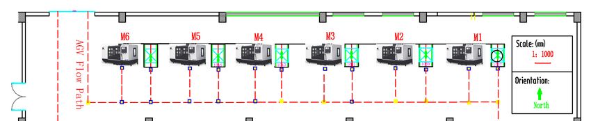
As shown in Figure 3, it is a layout of Hub workshop, which is a workshop of a robot
As shown in Figure 3, it is a layout of Hub workshop, which is a workshop of a robot manufacturer.
manufacturer. There are six machines, one automated warehouse and some AGVs are involved in
There are six machines, one automated warehouse and some AGVs are involved in the shop-floor.
the shop-floor.
Figure 3. The layout of the hub workshop.
Figure 3. The layout of the hub workshop.
The distance among the warehouse and machines are shown in Table 2.
Sensors 2020, 20, x; doi: FOR PEER REVIEW www.mdpi.com/journal/sensorsSensors 2020, 20, 4507 12 of 17
Table 2. The distance among the warehouse and machines. (m0 is warehouse, m1 ∼ m6 are machines).
Distance [m] m0 m1 m2 m3 m4 m5 m6
m0 0 40 46 52 60 66 75
m1 40 0 6 12 16 24 33
m2 46 6 0 12 18 24 33
m3 52 12 6 0 6 12 21
m4 60 18 12 6 0 6 15
m5 66 24 18 12 6 0 9
m6 75 33 27 21 15 9 0
In the SSF as described in this section, one hub is a job. Each job can be completed through a
specific sequence of production processes. One production process type refers to a task type. There are
five types of tasks in the manufacturing process: Cutting (CT), turning (TU), grinding (GR), drilling
(DR), and tapping (TA). As a service provider, there are six different processing equipment (CNC
machines). Each machine can provide five different types of services. Each machine can execute
manufacturing tasks with different service time expectations. The service time and power of the
machines are shown in Table 3.
Table 3. The distance between the warehouse and each machine.
Time [s]\
m0 m1 m2 m3 m4 m5 m6
Power [kW/h]
1CT 180\3.74 190\3.11 170\4.38 180\4.24 190\3.41 200\4.5 180\3.74
2TU 170\4.38 190\4.11 170\4.48 170\4.59 180\4.24 200\3.95 170\4.38
job 3GR 170\4.06 190\3.18 170\3.70 170\4.08 180\5.82 200\4.08 170\4.06
4DR 230\4.18 240\4.13 250\3.20 230\4.19 240\4.09 200\5.01 230\4.18
5TA 220\5.40 220\5.39 240\4.17 230\5.28 240\4.68 260\4.57 220\5.40
In dynamic job shops, the distribution of jobs arrival process closely follows a Poisson distribution.
Hence, the time between job arrivals closely follows an exponential distribution [5]. According to
the historical data of customer’s orders, the probability distribution of order arrival is analyzed.
The Poisson distribution is used to describe the random arrival orders in the SSF. Suppose 15 jobs
randomly arrive in 30 min. The job arrivals rate λ is equal to 0.5, respectively. Each job contains two
attributes of time: Arrival time and due date, denoted by jobk = (ak , dk ). The relationship between
the order arrival time and due date is denoted by dk = ak + c [5]. According to the production data of
the enterprise in three months, the average operation time of the jobs is 2000 s in the hub workshop,
therefore, c = 2000 s.
The idle energy consumption of the machine is shown in Table 4.
Table 4. Idle power of machines.
mi m0 m1 m2 m3 m4 m5 m6
Idle Power [kW/h] 0.98 1.23 1.48 1.06 1.06 1.16 1.27
The idle energy consumption of AGV is 0 because the communication cost is not considered in
this paper. The speed and handling power of AGVs are shown in Table 5.
Table 5. Power\speed of automated guided vehicle (AGVs).
AGV ai
Power [kW/h] 1
Speed [m/s] 0.5Sensors 2020, 20, 4507 13 of 17
The proposed method has been performed in python language on a computer with an Intel I7
4710MQ CPU 2.5 GHz processor and 8.00 GB memory.
6.2. Results of the Experiments
In order to illustrate the potential of the proposed method for the multi-objective dynamic JSP,
it is compared with the self-adaptive collaboration method (SCM) [33] and some common dispatching
rules. A combination decision model of scheduling rules such as the longest processing time (LPT)
dispatching rule, the shortest processing time (SPT) dispatching rule, and the first in first out (FIFO)
dispatching rule [5].
Paper [33] views each resource (machine and AGV) in the job shop as an active entity to request the
production tasks. The processing and logistics tasks will be allocated to the optimal resources according
to their real-time status by using the weight method. This method only considers the real-time status
of resources but does not fully consider the value engineering information such as random arrival jobs.
Therefore, sometimes the resources allocation may not be suitable, thereby reducing the efficiency
of the production system. Compared with the above research, which stands at the viewpoint of a
real-time job shop multi-resource self-organization in the production execution stage, our model stands
at the viewpoint of a real-time job shop multi-resource self-adaption for autonomous allocation of
SPLA in both production execution and customer requirements stage.
According to the case study, a series of experiments are conducted in order to evaluate the
contribution of the adaptive weight mechanism based on the entropy to the performance method.
Table 6 contains the average and standard deviation values for makespan, energy consumption,
and mean tardiness obtained across 200 runs on each instance with different numbers of AGVs.
With the increase of the number of AGVs, the indexes of all methods are improved. It can be easily
found from Table 6 that the proposed method has the potential to achieve the optimal solutions.
It also can be found in that the mean and variance of makespan, total energy consumption, and mean
tardiness of the proposed method are best among all the methods. Furthermore, it can also be seen
that the SPT performs better than the SCM, and the SCM performs better than the LPT. This is mainly
because compared with the SCM model, FIFO + SPT has a powerful predilection of time minimization,
which can handle complex relationships between more objectives, thus resulting in a relatively better
performance. However, the powerful predilection of time maximum of FIFO + LPT is hard to deal with
the interaction between multiple objectives, thus resulting in the worst performance. These results
illustrate that the proposed method performs better among all the methods, and it can improve the
performance of the scheduling system by keeping the schedule stability and the schedule efficiency
simultaneously when the jobs arrival at random.
According to the above analysis, we can observe that FIFO + LPT performs the worst. Therefore,
we will not cover it in this study. Figure 4 intuitively shows the three-dimensional Pareto fronts
obtained by three algorithms (i.e., RTSIET, FIFO + SPT, and SCM) with five AGVs in solving the
problem. It is clear that the non-dominated solutions obtained by RTSIET get closer to the coordinate
origin. In most cases, the solutions of SCM and FIFO + SPT are scattered, which means that SMC
and FIFO + SPT are challenging to obtain better results stably. It implies the superiority of RTSIET
compared with other algorithms in solving the proposed problem.
In order to verify the universality and effectiveness of the proposed method, we have also done a
simulation verification on other production workshops (e.g., bearing support workshop and assembly
workshop). Compared with other methods, the stability and effectiveness of the proposed method
are still the best. Since in the high disturbance production environment, the adaptive scheduling
strategy based on the information entropy can well balance time and energy consumption. The balance
characteristics of the proposed method has extraordinary significance for intelligent workshops:
(1) A good scheduling method can not only improve customer satisfaction and reduce production
costs, but also reduce the interference of human factors through replacing some of the functions of theSensors 2020, 20, 4507 14 of 17
workshop manager. (2) The stability and excellent scheduling results of the adaptive scheduling strategy
proves that the proposed method is an effective method to realize an intelligent unmanned workshop.
Table 6. Results comparison with the real-time scheduling algorithm based on the information entropy
theory (RTSIET), self-adaptive collaboration method (SCM), first in first out (FIFO) + longest processing
time (LPT), and FIFO + the shortest processing time (SPT).
RTSIET SCM
Sensors 2020, 20, x FOR PEER REVIEW 14 of 17
NA Cmax [s] E [10,000 J] T [s] Cmax [s] E [10,000 J] T [s]
MV V s] MV
[100 V J] MV [100Vs]
E [100,000 MV [s]V EMV V
[10,000 J] MV[s] V
1 MV
3898 179V 7857 MV 101V 108 MV 5V MV
5881 V
2893 MV
8763 V 1558 MV1932 V 143
2 1 3135
193 554.20 7416
1840 102
37.5 0197 6.37
0 5328
3918 2661
157 8195 127
8201 1259 1518 927118
1149
3 2 3040
192 724.17 7281
1828 9536.4 0196 6.36
0 5266
3559 2741
82 8089 121
7873 1314 1346 411122
965
4 3 2989
190 533.56 7204
1812 101
31.1 0193 5.54
0 5197
3498 2723
71 8014 115
7777 1328 1234 351124
784
5 4 2975
187 513.03 7165
1787 9027.8 0190 4.88
0 5202
3509 2695
73 7978 110
7769 1221 1004 363117
965
5 188 2.94 FIFO + LPT
1736 34.4 181 3.69 3639 79 FIFO +991
7761 SPT 857 371
Notes:
NA NA represents
Cmax [100 s] the number J]of AGVs;
E [100,000 E s]
T[100 represents total
Cmax [s] energyE consumption;
[10,000 J] represents
T[s]
mean tardiness; represents makespan; MV represents mean value; V represents variance.
MV V MV V MV V MV V MV V MV V
According
1 to the4.20
193 above1840
analysis,
37.5we can
197 observe
6.37 that FIFO157
3918 + LPT8201
performs127 the1149
worst. Therefore,
927
we will 2not cover
192 it 4.17
in this1828
study.36.4
Figure1964 intuitively
6.36 shows82the three-dimensional
3559 7873 121 965 Pareto
411 fronts
3 190 3.56 1812 31.1 193 5.54 3498 71 7777 115
obtained by three algorithms (i.e., RTSIET, FIFO + SPT, and SCM) with five AGVs in solving 784 351 the
4 187 3.03 1787 27.8 190 4.88 3509 73 7769 110 965
problem. It is clear that the non-dominated solutions obtained by RTSIET get closer to the coordinate 363
5 188 2.94 1736 34.4 181 3.69 3639 79 7761 991 857 371
origin. In most cases, the solutions of SCM and FIFO + SPT are scattered, which means that SMC and
NA represents the number of AGVs; E represents total energy consumption; T represents mean tardiness;
FIFONotes:
+ SPT are challenging to obtain better results stably. It implies the superiority of RTSIET
Cmax represents makespan; MV represents mean value; V represents variance.
compared with other algorithms in solving the proposed problem.
Figure 4.
Figure Pareto front
4. Pareto front of
of three
three algorithms
algorithms in
in solving
solving the
the proposed
proposed problem.
problem.
7. Conclusions
In order to verify the universality and effectiveness of the proposed method, we have also done
This
a simulation paper focuses on
verification on other
the enterprise’s
production manufacturing
workshops (e.g., decisions
bearing by considering
support workshop a high
and
disturbance environment. A real-time status model of heterogeneous resources in
assembly workshop). Compared with other methods, the stability and effectiveness of the proposed SSF is established.
The mathematical
method model
are still the best.is formulated
Since in thewith three
high objectives, production
disturbance i.e., the makespan, energy consumption,
environment, the adaptive
and
scheduling strategy based on the information entropy can well balance time and entropy
mean tardiness of jobs. A real-time scheduling algorithm based on the information energy
theory (RTSIET)
consumption. Thebased on characteristics
balance the dynamic service capabilitymethod
of the proposed of manufacturing resources
has extraordinary is proposed.
significance for
Then, a real-world
intelligent workshops:case(1)isAemployed to explore
good scheduling the scheduling
method can not onlymethod
improveincustomer
a high disturbance
satisfaction and
and
reduce production costs, but also reduce the interference of human factors through replacing some
of the functions of the workshop manager. (2) The stability and excellent scheduling results of the
adaptive scheduling strategy proves that the proposed method is an effective method to realize an
intelligent unmanned workshop.Sensors 2020, 20, 4507 15 of 17
multi-resource environment. In addition, the algorithm performance under random arrival jobs is
analyzed. The proposed model is solved by RTSIET, which can obtain the real-time multi-objective
weight value by calculating the standard information entropy of each job. The agility and stability of
the system are demonstrated through a practical application.
We will apply this real-time scheduling strategy to a combination of other methods in our future
research. The game theory may be a good candidate due to its multi-resource collaboration ability.
Author Contributions: W.Y. proposed the key idea for this paper and wrote the manuscript; W.L. reviewed the
manuscript and put forward constructive suggestions; Y.C. provided suggestions for organizing this manuscript
and polished it; Y.L. and L.H. helped with reviewing the manuscript. All authors have read and agreed to the
published version of the manuscript.
Funding: This research was funded by the Program for the Natural Science Foundation of China (NSFC) under
grant no. 61571336.
Conflicts of Interest: The authors declare no conflict of interest.
References
1. Rostami, M.; Kheirandish, O.; Ansari, N. Minimizing maximum tardiness and delivery costs with batch
delivery and job release times. Appl. Math. Model. 2015, 39, 4909–4927. [CrossRef]
2. Karimi-Nasab, M.; Seyedhoseini, S.M.; Modarres, M.; Heidari, M. Multi-period lot sizing and job shop
scheduling with compressible process times for multi-level product structures. Int. J. Prod. Res. 2013, 51,
6229–6246. [CrossRef]
3. Zhou, L.; Zhang, L.; Ren, L.; Wang, J. Real-Time Scheduling of Cloud Manufacturing Services Based on
Dynamic Data-Driven Simulation. IEEE T. Ind. Inform. 2019, 15, 5042–5051. [CrossRef]
4. Moghaddam, S.K.; Saitou, K. On optimal dynamic pegging in rescheduling for new order arrival.
Comput. Ind. Eng. 2019, 136, 46–56. [CrossRef]
5. Zhang, L.; Gao, L.; Li, X. A hybrid genetic algorithm and tabu search for a multi-objective dynamic job shop
scheduling problem. Int. J. Prod. Res. 2013, 51, 3516–3531. [CrossRef]
6. Wu, C.; Buyya, R.; Ramamohanarao, K. Modeling cloud business customers’ utility functions. Future Gener.
Comp. Syst. 2019, 12, 44. [CrossRef]
7. Marcin, C.; Jakub, N.A. Fast Genetic Algorithm for the Flexible Job Shop Scheduling Problem. In Proceedings
of the 2014 Conference Companion on Genetic and Evolutionary Computation Companion, Vancouver, BC,
Canada, 8–12 July 2014; pp. 1449–1450. [CrossRef]
8. Imran, A.; Khan, A.A. A research survey: Review of flexible job shop scheduling techniques. Int. Trans.
Oper. Res. 2016, 23, 551–591. [CrossRef]
9. Cao, Y.L.; Zhang, H.; Li, W.F.; Zhou, M.C.; Zhang, Y.; Chaovalitwongse, W.A. Comprehensive Learning Particle
Swarm Optimization Algorithm with Local Search for Multimodal Functions. IEEE Trans. Evol. Comput.
2018, 23, 718–731. [CrossRef]
10. He, L.J.; Li, W.F.; Zhang, Y.; Cao, Y.L. A discrete multi-objective fireworks algorithm for flowshop scheduling
with sequence-dependent setup times. Swarm Evol. Comput. 2019, 51, 100575. [CrossRef]
11. Reddy, K.S.; Panwar, L.K.; Kumar, R.; Panigrahi, B.K. Distributed resource scheduling in smart grid with
electric vehicle deployment using fireworks algorithm. J. Mod. Power Syst. 2016, 42, 188–199. [CrossRef]
12. Gu, X.L.; Huang, M.; Liang, X. A Discrete Particle Swarm Optimization Algorithm With Adaptive Inertia
Weight for Solving Multiobjective Flexible Job-shop Scheduling Problem. IEEE Access. 2020, 8, 33125–33136.
[CrossRef]
13. Ham, M.; Lee, Y.H.; Kim, S.H. Real-time scheduling of multi-stage flexible job shop floor. Int. J. Prod. Res.
2011, 49, 3715–3730. [CrossRef]
14. Ding, K.; Zhang, X.; Chan, F.T.S.; Chan, C.; Wang, C. Training a Hidden Markov Model-Based Knowledge
Model for Autonomous Manufacturing Resources Allocation in Smart Shop Floors. IEEE Access. 2019, 7,
47366–47378. [CrossRef]
15. Liu, X.F.; Shahriar, M.R.; Sunny, S.M.N. Cyber-physical manufacturing cloud: Architecture, virtualization,
communication, and testbed. J. Manuf. Syst. 2017, 43, 352–364. [CrossRef]Sensors 2020, 20, 4507 16 of 17
16. Ding, K.; Chan, F.T.S.; Zhang, X.; Zhou, G.; Zhang, F. Defining a Digital Twin-based Cyber-Physical
Production System for Autonomous Manufacturing in Smart Shop Floors. Int. J. Prod. Res. 2019, 57,
6315–6334. [CrossRef]
17. Yu, T.; Zhu, C.; Chang, Q.; Wang, J. Imperfect corrective maintenance scheduling for energy efficient
manufacturing systems through online task allocation method. J. Manuf. Syst. 2019, 53, 282–290. [CrossRef]
18. Kück, M.; Ehm, J.; Freitag, M.; Frazzon, E.M.; Pimentel, R. A data-driven simulation-based optimisation
approach for adaptive scheduling and control of dynamic manufacturing systems. Adv. Mat. Res. 2016, 1140,
449–456. [CrossRef]
19. Zhong, R.Y.; Dai, Q.Y.; Qu, T.; Hu, G.J.; Huang, G.Q. RFID-enabled real-time manufacturing execution system
for mass-customization production. Robot. CIM-Int. Manuf. 2013, 29, 283–292. [CrossRef]
20. Luo, Y.; Duan, Y.; Li, W.F.; Pace, P.; Fortino, G. Workshop Networks Integration Using Mobile Intelligence in
Smart Factories. IEEE Commun. Mag. 2018, 56, 68–75. [CrossRef]
21. Luo, Y.; Duan, Y.; Li, W.F.; Pace, P.; Fortino, G. A novel mobile and hierarchical data transmission architecture
for smart factories. IEEE Trans. Ind. Inform. 2018, 14, 3534–3546. [CrossRef]
22. Zhang, Y.F.; Huang, G.Q.; Sun, S.D.; Yang, T. Multi-agent based real-time production scheduling method for
radio frequency identification enabled ubiquitous shopfloor environment. Comput. Ind. Eng. 2014, 76, 89–97.
[CrossRef]
23. Shiue, Y.R.; Lee, K.C.; Su, C.T. Real-time scheduling for a smart factory using a reinforcement learning
approach. Comput. Ind. Eng. 2018, 125, 604–614. [CrossRef]
24. Zhang, Y.; Wang, J.; Liu, S.; Qian, C. Game Theory Based Real-Time Shop Floor Scheduling Strategy and
Method for Cloud Manufacturing. Int. J. Intell. Syst. 2016, 32, 437–463. [CrossRef]
25. Wang, J.; Zhang, Y.F.; Liu, Y.; Wu, N. Multiagent and Bargaining-Game-Based Real-Time Scheduling for
Internet of Things-Enabled Flexible Job Shop. IEEE Internet Things J. 2019, 6, 2518–2531. [CrossRef]
26. Qu, T.; Pan, Y.; Liu, X.; Kang, K.; Li, C.; Thurer, M.; Huang, G.Q. Internet of Things-based real-time production
logistics synchronization mechanism and method toward customer order dynamics. Trans. Inst. Meas. Control
2017, 39, 429–445. [CrossRef]
27. Bottani, E.; Centobelli, P.; Cerchione, R.; Gaudio, L.D.; Murino, T. Solving machine loading problem of
flexible manufacturing systems using a modified discrete firefly algorithm. Int. J. Ind. Eng. Comput. 2017, 8,
363–372. [CrossRef]
28. Miller-Todd, J.; Steinhöfel, K.; Veenstra, P. Firefly-Inspired Algorithm for Job Shop Scheduling. In Lecture
Notes Computer Science; Springer: New York, NY, USA, 2018; Volume 11011, pp. 423–433. [CrossRef]
29. Zhang, Y.; Qian, C.; Lv, J. Agent and Cyber-Physical System Based Self-Organizing and Self-Adaptive
Intelligent Shopfloor. IEEE Trans. Ind. Inform. 2017, 13, 737–747. [CrossRef]
30. Bányai, Á.; Illés, B.; Glistau, E.; Machado, N.I.C.; Tamás, P.; Manzoor, F.; Bányai, T. Smart Cyber-Physical
Manufacturing: Extended and Real-Time Optimization of Logistics Resources in Matrix Production. Appl. Sci.
2019, 9, 1287. [CrossRef]
31. Azadian, F.; Murat, A.; Chinnam, R.B. Integrated production and logistics planning: Contract manufacturing
and choice of air/surface transportation. Eur. J. Oper. Res. 2015, 247, 113–123. [CrossRef]
32. Zafarzadeh, M.; Hauge, J.B.; Wiktorsson, M.; Hedman, I.; Bahtijarevic, J. Real-Time Data Sharing in Production
Logistics: Exploring Use Cases by an Industrial Study. Int. Fed. Inf. Process. 2019, 567, 285–293. [CrossRef]
33. Szabolcs, D.; Sarbast, M. Examining Pareto optimality in Analytic Hierarchy Process on Real Data:
An Application in Public Transport Service Development. Expert Syst. Appl. 2019, 116, 21–30. [CrossRef]
34. Zhang, Y.F.; Guo, Z.G.; Lv, J.X.; Liu, Y. A Framework for Smart Production-Logistics Systems Based on CPS
and Industrial IoT. IEEE Trans. Ind. Inform. 2018, 14, 4019–4032. [CrossRef]
35. Gao, K.Z.; Suganthan, P.N.; Pan, Q.K.; Chua, T.J.; Cai, T.X.; Chong, C.S. Discrete harmony search algorithm for
flexible job shop scheduling problem with multiple objectives. J. Intell. Manuf. 2014, 27, 363–374. [CrossRef]
36. Vela, C.R.; Afsar, S.; Palacios, J.J.; González-Rodríguez, I.; Puente, J. Evolutionary tabu search for flexible
due-date satisfaction in fuzzy job shop scheduling. Comput. Oper. Res. 2020, 119, 305–548. [CrossRef]
37. Lu, Y.; Xu, X. Resource virtualization: A core technology for developing cyber-physical production systems.
J. Manuf. Syst. 2018, 47, 128–140. [CrossRef]
38. Järvenpää, E.; Lanz, M.; Siltala, N. Formal Resource and Capability Models supporting Re-use of
Manufacturing Resources. Procedia Manuf. 2018, 19, 87–94. [CrossRef]You can also read