My journal manuscript No. (will be inserted by the editor) Deep Reinforcement Learning for Constrained Field Development Optimization in ...
←
→
Page content transcription
If your browser does not render page correctly, please read the page content below
my journal manuscript No.
                                         (will be inserted by the editor)

                                         Deep Reinforcement Learning for Constrained Field Development Optimization in
                                         Subsurface Two-phase Flow

                                         Yusuf Nasir2 · Jincong He1 · Chaoshun Hu1 ·
                                         Shusei Tanaka1 · Kainan Wang1 · XianHuan Wen1
arXiv:2104.00527v1 [cs.LG] 31 Mar 2021

                                         Received: date / Accepted: date

                                         Abstract Oil and gas field development optimization, which involves the determination of the
                                         optimal number of wells, their drilling sequence and locations while satisfying operational and
                                         economic constraints, represents a challenging computational problem. In this work, we present
                                         a deep reinforcement learning-based artificial intelligence agent that could provide optimized de-
                                         velopment plans given a basic description of the reservoir and rock/fluid properties with minimal
                                         computational cost. This artificial intelligence agent, comprising of a convolutional neural net-
                                         work, provides a mapping from a given state of the reservoir model, constraints, and economic
                                         condition to the optimal decision (drill/do not drill and well location) to be taken in the next stage
                                         of the defined sequential field development planning process. The state of the reservoir model is
                                         defined using parameters that appear in the governing equations of the two-phase flow (such as
                                         well index, transmissibility, fluid mobility, and accumulation, etc.).
                                             A feedback loop training process referred to as deep reinforcement learning is used to train
                                         an artificial intelligence agent with such a capability. The training entails millions of flow simula-
                                         tions with varying reservoir model descriptions (structural, rock and fluid properties), operational
                                         constraints (maximum liquid production, drilling duration, and water-cut limit), and economic
                                         conditions. The parameters that define the reservoir model, operational constraints, and economic
                                         conditions are randomly sampled from a defined range of applicability. Several algorithmic treat-
                                         ments are introduced to enhance the training of the artificial intelligence agent. After appropriate
                                         training, the artificial intelligence agent provides an optimized field development plan instantly
                                         for new scenarios within the defined range of applicability. This approach has advantages over
                                         traditional optimization algorithms (e.g., particle swarm optimization, genetic algorithm) that are
                                         generally used to find a solution for a specific field development scenario and typically not gen-
                                         eralizable to different scenarios. The performance of the artificial intelligence agents for two- and
                                         three-dimensional subsurface flow are compared to well-pattern agents. Optimization results using
                                         the new procedure are shown to significantly outperform those from the well pattern agents.
                                         Corresponding author: Yusuf Nasir
                                         E-mail: nyusuf@stanford.edu

                                         1   Chevron ETC

                                         2   Stanford University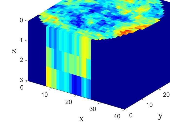
2                                                Y. Nasir, J. He, C. Hu, S. Tanaka, K. Wang, X. Wen

    Compared to prior work on this topic such as He et al. (2021), the novelties in this work include:
– Extended the problem description from single-phase flow to two-phase flow, and thus allowing
  for handling of reservoirs with strong aquifers and waterflooding problems.
– Redesigned deep network neural network architecture for better performance.
– Extended to handle operational constraints such as maximum liquid production, drilling dura-
  tion and water-cut limit.
– Extended to three-dimensional reservoir model.

1 Introduction

Field development decisions such as the number of wells to drill, their location and drilling se-
quence need to be made optimally to maximize the value realized from a petroleum asset. Op-
timization algorithms such as evolutionary strategies are, in recent times, widely applied to the
field development optimization problem (Isebor et al. 2014b,a). However, the application of these
optimization algorithms is challenging due to the very large number of computationally expensive
flow simulations required to obtain optimal (or near optimal) solutions. In addition, the field de-
velopment optimization problem is typically solved separately for each petroleum field due to the
variation in geological model, constraints to be considered or even the economic condition. Thus,
the large number of computationally expensive flow simulations needs to be run for each field
under consideration. This suggests the field development optimization problem will benefit from
strategies that would allow for the generalization of the optimization process to several petroleum
fields.
    In our recent work He et al. (2021), we developed a deep reinforcement learning technique for
the field development optimization in two-dimensional subsurface single-phase flow settings. The
deep reinforcement learning technique allows for the training of an artificial intelligence agent that
provides a mapping from the current state of a two-dimensional reservoir model to the optimal de-
cision (drill/do not drill and well location) in the next step of the development plan. Our goal in this
work is to extend the procedures in He et al. (2021) for the field development optimization, in the
presence of operational constraints, in both two- and three-dimensional subsurface two-phase flow.
Once properly trained, the artificial intelligence agent should learn the field development logic and
provide optimized field development plans instantly for different field development scenarios. Be-
sides the described extensions to more complex simulation models, several algorithmic treatments
are also introduced in this work to enhance the training of the artificial intelligence agent under the
deep reinforcement learning framework.
    In the literature of oil and gas field development and production optimization, different opti-
mization algorithms have been applied to solve different aspects of the optimization problem. The
well control or production optimization problem in which the time-varying operational settings of
existing wells are optimized has been efficiently solved with gradient-based methods (Brouwer and
Jansen 2002; Sarma et al. 2006; Echeverria Ciaurri et al. 2011; Awotunde 2019), ensemble-based
methods (Fonseca et al. 2014; Chen et al. 2009) or with efficient proxies like reduced-order mod-
els (Cardoso and Durlofsky 2010; He et al. 2011). For the well placement optimization, popular al-
gorithms such as the genetic algorithms and the particle swarm optimization algorithms (Bangerth
et al. 2006; Onwunalu and Durlofsky 2010; Bouzarkouna et al. 2012; Isebor et al. 2014b,a) typ-
ically entail thousands of simulation runs to get improved result with no guarantee of global op-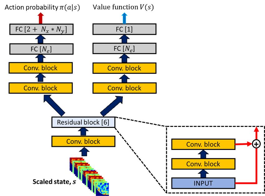
DRL for Constrained FDO                                                                              3

timality. The joint well placement and production optimization problems have also been consid-
ered (Zandvliet et al. 2008; Bellout et al. 2012; Isebor et al. 2014a,b; Nasir et al. 2020), which
typically require even larger numbers of simulations. In addition, while the approaches considered
in these studies may provide satisfactory results for the field development optimization problem,
the solution obtained in each case is tied to a specific field development scenario. If the economic
conditions or geological models used in the optimization change, the optimization process needs
to be repeated. In other words, the solution from traditional optimization methods lacks the ability
to generalize when the underlying scenario changes. It should be noted that the ability to general-
ize that is discussed here is different from the robust optimization as studied in Chen et al. (2012,
2017), in which the optimization is performed under uncertainty. While the solutions from robust
optimization accounts for the uncertainty in the the model parameters, they still don’t generalize
when the ranges of those uncertainties change.
    In this work, we consider the reinforcement learning technique in which a general AI (in the
form of a deep neural network) can be applied to optimize field development planning for a range of
different scenarios (e.g., different reservoir, different economics, different operational constraints)
once it is trained. The reinforcement learning technique considered in this work for the field devel-
opment optimization problem has shown great promise in other fields. Google DeepMind trained
an artificial intelligence agent AlphaGo (Silver et al. 2016) using reinforcement learning with a
database of human expert games. AlphaGo beat the human world champion player in the game of
Go. AlphaGo Zero (Silver et al. 2017a) which is a variant of AlphaGo was trained through self-play
without any human knowledge. AlphaGo Zero defeated AlphaGo in the game of Go. In AlphaGo
and AlphaGo Zero, the AI takes in a description of the current state of the Go game and chooses an
action to take for the next step. The choice of action is optimized in the sense that it maximizes the
overall probability of winning the game. The success of AlphaGo and AlphaGo Zero suggests the
possibility of training an AI for field development that takes in a description of the current state of
the reservoir and chooses the development options (e.g., drilling actions) for the next step, without
prior reservoir engineering knowledge.
    In the petroleum engineering literature, deep learning algorithms have seen much success re-
cently for constructing proxies for reservoir simulation models (Wang et al. 2021; Jin et al. 2020;
Tang et al. 2021). Reinforcement learning algorithms have been applied to solve the production op-
timization problem for both steam injection in steam-assisted gravity drainage (SAGD) recovery
process (Guevara et al. 2018) and waterflooding (Hourfar et al. 2019). Deep reinforcement learning
(in which the artificial intelligence agent is represented by a deep neural network) has also been
applied to the production optimization problem (Ma et al. 2019; Miftakhov et al. 2020). Ma et al.
(2019) evaluated the performance of different deep reinforcement learning algorithms on the well
control optimization problem with fully connected neural networks (FCNN). The state of the reser-
voir model defined by two-dimensional maps are flattened and used as input to the FCNN and thus
do not retain the spatial information inherent in the data. An FCNN-based artificial intelligence
agent was also trained in Miftakhov et al. (2020). It should be noted that in the studies discussed
here, the reinforcement learning process is used as a replacement for traditional optimization al-
gorithms (such as particle swarm optimization, genetic algorithm) to optimize a predefined field
development scenario.
    He et al. (2021) applied the deep reinforcement learning technique to the more challenging
field development optimization problem in which the decisions to be made include the number of
wells to drill, their locations, and drilling sequence. In contrast to the previous studies discussed,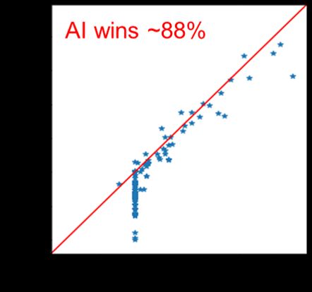
4                                               Y. Nasir, J. He, C. Hu, S. Tanaka, K. Wang, X. Wen

He et al. (2021) used DRL to develop artificial intelligence which could provide optimized field
development plans given any reservoir description within a predefined range of applicability. In
addition, unlike in previous studies (Ma et al. 2019; Miftakhov et al. 2020) in which the artificial
intelligence agent is represented by fully connected neural networks, He et al. (2021) utilized a
convolutional neural network to represent the agent which allows for better processing of spatial
information. The field development optimization problem in He et al. (2021), however, considers
a single-phase flow in two-dimensional reservoir models.
    In this paper, we build upon He et al. (2021) and formulate deep reinforcement learning-based
artificial intelligence agents that could provide optimized field development plans instantaneously
based on the description of a two- or three-dimensional subsurface two-phase flow in the presence
of operational constraints. The sequence of actions to take during the field development process
is made by the artificial intelligence agent after processing the state of the reservoir model, the
prescribed constraints and economic condition. The state of the reservoir model in this work is
defined using parameters that appear in the governing equations of the two-phase flow (such as
pressure, saturation, well index, transmissibility, fluid mobility, and accumulation). We also pro-
pose a dual-action probability distribution parameterization and an improved convolutional neural
network architecture to enhance the training efficiency of the artificial intelligence agents for the
field development optimization problem.
    This paper proceeds as follows. In Section 2, we present the governing equations for the two-
phase flow and discuss the different field development optimization approaches – traditional and
reinforcement learning-based field development optimization. In Section 3, we present the deep
reinforcement learning field development approach which includes the state and action represen-
tation, the proximal policy algorithm and the deep neural network used to represent the policy and
value functions of the agent. Computational results demonstrating the performance of the deep re-
inforcement learning agents, for both 2D and 3D problems, are presented in Section 4. We conclude
in Section 5 with a summary and suggestions for future work.

2 Governing Equations and Field Development Optimization Approaches

In this section, we first briefly discuss the governing equations for the two-phase flow. We then de-
scribe the traditional and reinforcement learning-based field development optimization approaches.

2.1 Governing equations

In this work, we consider the isothermal immiscible oil-water flow problem with gravitational
effects. Combining Darcy’s law for multiphase flow and the mass conservation equation while
neglecting capillary pressure, the flow of each phase in the reservoir can be described using:
                               h                   i ∂
                           ∇ · kρl λl (∇p − γl ∇D) = (φ ρl Sl ) + ql ,                         (1)
                                                        ∂t
where the subscript l represents the phase (l = o for oil and l = w for water), k is the permeability
tensor, ρl is the phase density, λl = kr,l /µl is the phase mobility, with kr,l the phase relative per-
meability and µl the phase viscosity, p is the pressure (with p = po = pw since capillary pressure
is neglected), γl = ρl g is the phase specific weight, with g the gravitational acceleration, D is the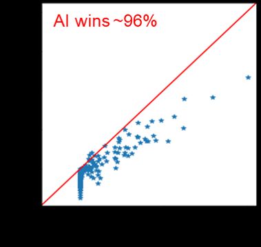
DRL for Constrained FDO                                                                                 5

depth, φ is the porosity, Sl is the phase saturation and ql is the mass sink term. The phase flow rate
for a production well w in well-block i is defined by the Peaceman well model (Peaceman 1983):

                                        (qw                            w
                                          l )i = W Ii (λl ρl )i (pi − p ),                            (2)
where W Ii is the well-block well index which is a function of the well radius, well block geometry
and permeability, pi denotes the well block pressure and pw denotes the well bottomhole pressure.
    The discretized form of Eq. 1 given in Eq. 3 is solved for each grid block i, in time, using the
fully implicit method.

                                                   pn+1 − pni

                                (ct )l φV Sl        i
                                                              = ∑ Γl k ∆Ψlk + (ql )i ,                (3)
                                     Bl        i      ∆t        k
where pi the pressure of grid block i, n and n + 1 indicate the time levels, V is the volume of the
grid block, (ct )l denotes the total phase compressibility of the grid block, Bl is the phase formation
volume factor of the grid block, k represents an interface connected to grid block i, ∆Ψlk is the
difference in phase potential over the interface k, Γl k = Γ k λlk is the phase transmissibility over the
interface k, with Γ k the rock transmissibility which is a function of the permeability and geometry
of the grid blocks connected by interface k.

2.2 Optimization problem formulation and traditional approaches

The aim in the field development optimization problem in this work is to determine the number
of wells to drill in a greenfield, alongside their locations and drilling sequence. Only the primary
depletion mechanism is considered, thus all wells to be drilled are production wells. The constraints
imposed on the field development include the maximum liquid production rate, drilling duration
for each well, the allowable water cut limit, and minimum inter-well spacing.
   Mathematically, the field development optimization problem can be written as follows:
                                       max J(x), subject to c(x) ≤ 0,                                 (4)
                                       x∈X

where J is the objective function to be optimized, the decision vector x ∈ X defines the number
of wells to drill, their locations, and drilling sequence. The space X defines the feasible region
(upper and lower bounds) for the decision variables. The vector c defines optimization constraints
that should be satisfied. Interested readers can refer to Isebor et al. (2014a,b) for possible ways of
parameterizing the decision vector x for the field development optimization problem.
    The net present value (NPV) is typically considered as the objective function to be maximized
in the field development optimization. Thus, J in Eq. 4 can be specified as the NPV. The NPV for
primary depletion (only production wells) can be computed as follows:
                                    "N                                              #
                              T        w,p,t                             Nw,d,t
                 NPV(x) = ∑ γ tk ∑ (po − copex ) qio,k − c pw qiw,k − ∑ cw ,                       (5)
                             t=0         i=1                                             i=1

Here Nt is the number of time steps in the flow simulation, Nw is the number of production wells, tk
and ∆tk are the time and time step size at time step k, ti is the time at which producer i is drilled, and
po , copex and c pw represent the oil price, operating cost and the cost of produced water, respectively.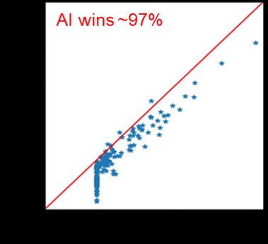
6                                                 Y. Nasir, J. He, C. Hu, S. Tanaka, K. Wang, X. Wen

The variables cw and γ represent the well drilling cost and annual discount rate, respectively. The
rates of oil and water production for well i at time step k are, respectively, qio,k and qiw,k .
    In the traditional approach of solving the field development optimization problem, the field de-
velopment scenario of interest is first defined. These include the reservoir model definition (struc-
tural, rock, and fluid properties), the specific constraints and the economic condition to be consid-
ered. Afterward, the optimization variables that define the number of well, location, and drilling
sequence are parameterized to obtain a formulation of x. Finally, an optimizer (e.g. particle swarm
optimization or genetic algorithm) iteratively proposes sets of decision variables (that represent
field development plans and are evaluated with a reservoir simulator) in order to maximize an
economic metric of interest. The optimized set of decision variables is tied to a particular field
development scenario predefined before the flow simulation.
    In the traditional approach, the evaluation of Eq. 5 for each field development plan requires
performing the two-phase flow simulation which involves solving Eq. 3. From those simulations,
the only information used by the traditional optimization approach is the corresponding NPV. The
reservoir states at each time step, which contain a lot of useful information, are discarded.
    Different from the traditional optimization approach, Reinforcement learning makes use of the
intermediate states generated from the simulator and provides optimized policy applicable to a
range of different scenarios.

2.3 Reinforcement learning-based field development optimization

Reinforcement learning is a sub-field of machine learning concerned with teaching an artificial
intelligence agent how to make decisions so as to maximize the expected cumulative reward. The
training and the decision making process of the AI agent follows a feedback paradigm as shown in
Fig. 1.

     Fig. 1: The reinforcement learning feedback loop (adapted from Sutton and Barto 2018).

    The reinforcement learning problem can be expressed as a system consisting of an agent and
an environment. The agent and the environment interact and exchange signals. These signals are
utilized by the agent to maximize a given objective. The exchanged signals, also referred to as
experience, are (st , at , rt ), which denotes the state, action, and reward respectively. Here, t defines
the time step in which the experience occurred. At a given stage t of the decision-making process,
with the environment (which represents where the action is taken) at state st , the agent takes an
action or decision at . The quality of the action at is quantified and signaled to the agent through
the reward rt . The decision-making process then transits to a new state st+1 which indicates the
DRL for Constrained FDO                                                                                 7

effect of action at on the environment. The transition from st to st+1 in reinforcement learning is
formulated as a Markov decision process (MDP) – which assumes the transition to the next state
st+1 only depends on the previous state st and the current action at . This assumption is referred
to as the Markov property (Howard 1960). The feedback loop terminates at a terminal state or a
maximum time step t = T . The time horizon from t = 0 to when the environment terminates is
referred to as an episode.
   The choice of the action to take at stage t by the agent depends on the observation ot which is a
function of st . If ot contains all the information in st , then the decision making process is referred
to as fully observable MDP. Otherwise, it is referred to a partially observable MDP (POMDP).
The agent’s action-producing function is referred to as a policy. Given a state st (relayed to the
agent through ot ), the policy produces the action at . This mapping operation is mathematically
represented as π(at | ot , θ ), where θ are the parameters that define the policy function. The rein-
forcement learning problem is now essentially an optimization problem with the goal of finding the
optimal policy parameters (θ opt ) that maximizes an expected cumulative reward. This optimization
problem is posed as:

                                                         "              #
                                                             T
                                     θ opt = arg max E       ∑ γ t rt   ,                             (6)
                                                 θ        t=0

where the reward at time t, rt = R(st , at , st+1 ) depends on the reward function R and γ ∈ [0, 1] is the
discount factor that accounts for the temporal value of rewards. The expectation accounts for the
stochasticity that may exist in the action and environment. If the parameters of the policy function
are the weights of a deep neural network, then the optimization problem is referred to as a deep
reinforcement learning (described in details later).
   In the context of field development optimization, our goal is to determine the policy function
that maximizes the expected NPV. At each drilling stage, the agent defines the action to be taken,
which includes whether to drill a producer or not and, if drill, the optimal well location. The envi-
ronment, which is the reservoir simulator, advances the flow simulation to the next drilling stage
by solving the governing equation for the immiscible oil-water system given in Eq. 1. The reward
function R for the reinforcement learning-based field development optimization problem is given
by the NPV (Eq. 5), where the reward for a drilling stage t is given by NPVt = NPV(st , at , st+1 ).
Here, NPV(st , at , st+1 ) defines the NPV obtained if the flow simulation starts from state st (includ-
ing all wells drilled from s0 to st ) and ends at state st+1 . It should be noted that since the NPV
defined in Eq. 5 accounts for discounting, we specify the the discount factor γ = 1 in Eq. 6.
   The formulation of the RL-based field development optimization in this work allows the ex-
ploitation of the problem states (st ) generated during the simulation and is thus a more efficient
use of the information from the potentially expensive simulation runs. In addition, the output of
the RL-based approach is not the optimal actions itself, but the optimal policy, a mapping from
the states to the optimal actions π(at |ot , θ ), which can be used obtain the optimal actions under
various different scenarios. This is distinctively different from the use of RL in Ma et al. (2019);
Miftakhov et al. (2020), where the goal was the optimal actions rather than the policy.
8 Y. Nasir, J. He, C. Hu, S. Tanaka, K. Wang, X. Wen
3 Deep Reinforcement Learning for Field Development Optimization
In this section, we present the deep reinforcement learning approach for field development opti-
mization where the parameters (θ ) of the policy function are defined by the weight of a convolu-
tional neural network. We first describe the action and state representation for the field development
optimization problem. Finally, the training procedure of the agent using the proximal policy opti-
mization algorithm (Schulman et al. 2017) and the convolutional neural network architecture are
described.
3.1 Action representation
The action representation is important because it affects the computational complexity of the learn-
ing process. At each drilling stage, the agent needs to decide to drill a well at a certain location or
not drill at all. We introduce two variables to make these decisions. The drill or do not drill decision
at drilling stage t is represented by a binary categorical variable wt ∈ {0, 1} where 0 represents the
decision not to drill a well and 1 the decision to drill. The second variable (active only when the
agent decides to drill a well, i.e. wt = 1) defines where the well should be drilled and is represented
by the well location variable ut , which is chosen from the possible drilling locations denoted by
u ∈ ZNx Ny (the 2D grid flattened into 1D), where Nx and Ny represents the number of grid blocks
in the areal x and y directions of the reservoir model. Each index in u maps to a grid block in the
reservoir model. Thus, at each drilling stage t, the action at is defined by at = [wt , ut ], where ut is
only considered if wt = 1.
The action representation used in this work differs from that used in He et al. (2021). Specifi-
cally, in He et al. (2021) a single variable of dimension Nx × Ny + 1 is used to define the possible
actions at each drilling stage, where the additional index represents the do-not-drill decision. Such
an action parameterization means the action at at each drilling stage is sampled from a single
probability distribution of cardinality Nx × Ny + 1. Thus, the do-not-drill decision depends on the
number of possible well locations (Nx × Ny ). As the size of the reservoir model increases, it be-
comes increasingly difficult for the agent to learn when not to drill a well due to the cardinality
of the probability distribution dominated by possible drilling locations. This is in contrast to the
approach used in this work where the variables wt and ut are sampled from two different proba-
bility distributions of cardinality 2 and Nx × Ny , respectively. Hence, the drill or do-not-drill action
is independent of the size of the reservoir model. The parameterization used in this work can be
naturally extended to other field development cases. For example, for waterflooding, the decision
on the well type can be incorporated in wt as wt ∈ {−1, 0, 1}, where -1 represents the decision to
drill an injector, 0 to not drill a well, and 1 to drill a producer.
Given the vector u, drilling in some grid blocks may lead to an unacceptable field development
plan from an engineering standpoint. These include field development plans where more than one
well is to be drilled in the same location, violation of minimum inter-well distance constraint (ac-
ceptable spacing between wells) and/or drilling in inactive regions of the reservoir. At any given
drilling stage, an action mask of the same dimension with u defines acceptable drilling locations
that the agent could choose from. Specifically, the probability of sampling an invalid drilling loca-
tion in u is set to zero. This action masking technique (Huang and Ontañón 2020; Tang et al. 2020)
have been proven to be an effective strategy to improve the convergence of the policy optimiza-
tion and also ensures the agent only takes valid action. The action masking technique was usedDRL for Constrained FDO 9
in He et al. (2021) for the field development optimization problem to ensure only feasible drilling
locations are proposed by the agent.
3.2 State representation
The definition of the state of the environment for the field development optimization problem
depends on the model physics. For example, the state would include pressure for single-phase flow
and, additionally, saturation for two-phase flow. The definition of the state also depends on the kind
of generalization capability that we want the AI to have. For example, if we want the AI to provide
different optimal solutions for different geological models, geological structures and properties
such as permeability, porosity should also be included in the state definition. If we want the AI to
be able to provide different optimal solutions under different oil prices, the oil price should also be
part of the state.
Our goal in this work is to develop an AI for two-phase flow that can provide optimal solutions
for different field development optimization scenarios with variable reservoir models, operational
constraints, and economic conditions within a predefined range. Thus, this variation in the scenar-
ios should be captured in the state representation.
In this work, the field development optimization scenarios considered are characterized by pa-
rameters following the distributions listed in Table 1. Each scenario defines a given geological
structure, rock and fluid properties, operational constraints, and economic conditions. This includes
the grid size, the spatial distribution of the grid thickness obtained through Sequential Gaussian
simulation (SGS) with a fixed mean, standard deviation, and variogram ranges. The porosity fields
which are also generated using SGS have a variable variogram structure and azimuth. A cloud
transform of the porosity field is used to generate the permeability and initial saturation fields.
After appropriate training, the AI agent is expected to provide an optimized field development
plan for an optimization scenario randomly sampled from this defined range of parameters. The
generalization and applicability of the resulting AI agent will depend on the optimization problem
parameters and their distributions. The number of learnable parameters of the neural network and
computational complexity of the training process of the AI increases as more parameters and larger
distributions are considered.
As pointed out in He et al. (2021), the parameters listed in Table 1 do no affect the model in-
dependently. Using them directly as input to the deep neural network increase the complexity and
the ill-conditioning of the problem. Therefore, we define the state of the environment using param-
eter groups that aid in reducing the number of input channels provided to the artificial intelligence
agent. These input channels include parameter groups that appear in the discretized form of the oil-
water immiscible flow problem (Eq. 3) and the reward. Additional input channels are also included
to define the operational constraints imposed on the field development. The constraints considered
include the drilling duration per well, watercut limit and the maximum well liquid production rate.
The list of input channels used to define the state of the environment are given in Table 2.
There are 17 input channels considered for the 2D subsurface system while 18 (including the
z-directional tramsmissibility) are used for the 3D system. The observation at any given drilling
stage (ot ) is represented by ot ∈ RNx ×Ny ×Nc , where Nc defines the number of channels. For the
2D case Nc = 17, where each scalar property (such as the drilling time or water cut constraint)
is converted to a 2D map of constant value. Out of the 18 input channels for the 3D system, 1010 Y. Nasir, J. He, C. Hu, S. Tanaka, K. Wang, X. Wen
Number Variable Symbol Distribution
1 Grid size in x-direction (ft) dx U[500, 700]
2 Grid size in y-direction (ft) dy U[500, 700]
3 Grid thickness (ft) dz SGS(1000,100,30,60)
4 Variogram azimuth (0 ) ang U[0, 90]
5 Variogram structure struct {Gaussian, exponential}
6 Porosity φ SGS(U[0.15,0.25],U[0.01,0.07],2,8)
7 Permeability (md) k cloud transform from φ
8 Vertical to horizontal permeability ratio (3D) kvkh logUnif[0.001, 0.1]
9 Active cell indicator active Random elliptical
10 Datum depth (ft) ddatum U[5000, 36000]
11 Depth from datum (ft) D SGS(1000,1000,30,60)
12 Pressure gradient (psi/ft) pgrad U[0.7, 1]
13 Initial water saturation Swinit cloud transform from φ
14 Oil reference formation volume factor Bo,re f U[1, 1.5]
15 Water reference formation volume factor Bw,re f U[1, 1.5]
16 Oil compressibility (psi−1 ) co U[1e-6, 4e-6]
17 Water compressibility (psi−1 ) cw U[2e-6, 5e-6]
18 Oil specific gravity γo U[0.8, 1]
19 Water density (lbs/ft3 ) ρw U[62, 68]
20 Oil reference viscosity (cp) µo,re f U[2, 15]
21 Water reference viscosity (cp) µw,re f U[0.5, 1]
22 Residual oil saturation Sor U[0.05, 0.2]
23 Connate water saturation Swc U[0.05, 0.2]
24 Oil relative permeability endpoint kroe U[0.75, 0.95]
25 Water relative permeability endpoint krwe U[0.75, 0.95]
26 Corey oil exponent no U[2, 4]
27 Corey water exponent nw U[2, 4]
28 Producer BHP (% pressure at datum) p w U[0.3, 0.7]
29 Producer skin s U[0, 2]
30 Oil price per bbl ($) po U[40, 60]
31 Water production cost (% oil price) cwp U[0, 0.02]
32 Operating cost per bbl ($) copex U[8, 15]
33 Drilling cost per well ($) ccapex U[1e8, 5e8]
34 Discount rate (%) b U[9, 11]
35 Drilling time per well (days) dtime {90, 120, 180, 240}
36 Project duration (years) ptime U[15, 20]
37 Watercut limit (%) wclimit U[60, 98]
38 Max. well liquid production rate (bbl/day) ql,max U[1e4, 2.5e4]
Table 1: Distribution of parameters for 2D and 3D oil-water system field development optimiza-
tion. U[a, b] denotes uniform distribution over the range of [a, b]. {a1 , a2 , · · · , an } indicate uniform
probability distribution over the n discrete options.DRL for Constrained FDO 11
(e.g. pressure, saturation, well index, e.t.c) vary spatially and thus the values for each layer of the
reservoir model is included in the input channel. This means in the 3D case, Nc = 10Nz + 8, where
Nz is the number of layers in the 3D reservoir model.
Once an optimization scenario is defined during training, the static input channels are computed
and saved. After advancing the flow simulation to any given drilling stage, the dynamic properties
are extracted and stacked with the static properties. This stacked input channels are then provided
to the agent as the state of the environment at that given drilling stage. In order to improve the
efficiency of the training process, all the input channels (except for the well location mask that is
zero everywhere and 1 only at regions where wells are located) are normalized to be very close to
0 to 1 range. Due to the highly skewed distribution of the transmissibilities and well index, they
are scaled with a nonlinear scaling function as done in He et al. (2021). Other input channels are
scaled using the linear min-max scaling function.
Number Input Channel Static/Dynamic
1 Pressure Dynamic
2 Water saturation Dynamic
3 x-directional transmissibility Static
4 y-directional transmissibility Static
5 z-directional transmissibility (3D) Static
6 Oil Accumulation Dynamic
7 Water mobility Dynamic
8 Oil mobility Dynamic
9 Well index Static
10 Producer drawdown Dynamic
11 Well location mask Dynamic
12 Well cost to net oil price ratio Static
13 Water production cost Static
14 Current discount rate Dynamic
15 Remaining production time Dynamic
16 Max. liquid production rate Static
17 Drilling time Static
18 Water cut constraint Static
Table 2: List of the input channels used to define the state for 2D and 3D oil-water system field
development optimization
3.3 Proximal policy optimization
Our goal is to determine the learnable parameters (defined by the weights of a neural network) of
the policy function that maximizes the expected cumulative reward as posed in the optimization
problem given in Eq. 6. In this work, we use a policy gradient method in which the expected
cumulative reward is maximized by performing gradient descent on the parameters of the policy.12 Y. Nasir, J. He, C. Hu, S. Tanaka, K. Wang, X. Wen
The vanilla policy gradient method is susceptible to performance deterioration due to the instability
that may be introduced by the update step during gradient descent. Several variants of the policy
gradient method have been proposed to improve the stability of the optimization. Some variants of
the policy gradient method include the trust region policy optimization (TRPO) (Schulman et al.
2015a) and proximal policy optimization (PPO) (Schulman et al. 2017).
The PPO algorithm proposes a surrogate objective that improves the policy optimization by
guaranteeing monotonic policy improvement. Following He et al. (2021), we now briefly describe
the implementation of PPO used in this work.
The PPO loss or objective function given in Eq. 7 contains four components: the surrogate
policy loss (Lπ ), the Kullback–Leibler (KL) divergence penalty (Lkl ), the value function loss (Lv f ),
and the entropy penalty (Lent ).
LPPO = Lπ + ckl Lkl + cv f Lv f + cent Lent (7)
where ckl , cv f and cent are user-defined weighting factors for the KL divergence, value function
and entropy terms, respectively.
The surrogate policy loss (Lπ ) that directly maximizes the expected cumulative reward is given
by:
Lπ = Et [min(rt (θ )At , clip(rt (θ ), 1 − ε, 1 + ε)At )] (8)
where rt (θ ) quantifies the policy change and it is defined as the ratio of the old policy π(at |st , θold )
to the new policy π(at |st , θ ). The term clip(rt (θ ), 1 − ε, 1 + ε) removes the incentive to change the
policy beyond a pre-defined step size limit ε. This prevents large updates of the parameters that
could lead to deterioration of the policy. The advantage function At defines how good an action is
for a specific state relative to a baseline. Following the generalized advantage estimation (GAE)
framework proposed by Schulman et al. (2015b), At is defined by:
T
GAE(γ,λ )
At (t) = ∑ (γλ )l−t (rl + γV π (sl+1 ) −V π (sl )) (9)
l=t
where γ and λ are hyperparameters that control the bias and variance introduced by the various
terms in the summation. The value function V π (st ), given in Eq. 10, represents the expected total
reward of being in state st and then following the current policy π. The value function is parame-
terized by the weights of a neural network ψ.
" #
T
V π (st ) = E ∑ rl (10)
l=t
The value function is learned by minimizing the value-function loss Lv f which is given by:
h 2 2 i
Lvf = Et max Vψ (st ) −Vtarget (st ) , Vψold + clip(Vψ (st ) −Vψold (st ), −η, η) −Vtarget (st ) ,
(11)
where the Vtarget (st ) is the computed value function from the training samples, Vψold is the value
function using the current parameters of the value function ψold . Equation 11 essentially tries to
minimize the mismatch between the computed and predicted value of the sampled states. TheDRL for Constrained FDO 13
hyperparameter η has same effect as ε in Eq. 8 and is used to ensure large updates of the value
parameters ψ are not allowed.
The KL divergence penalty (Lkl ) serves as an additional term to avoid large policy update and
it is given by:
LKL = Et [DKL (π(at |st , θ )|π(at |st , θold ))] , (12)
where DKL (π(at |st , θ )|π(at |st , θold )) is the Kullback–Leibler divergence (Kullback and Leibler
1951) that measures the difference between the old and new policy.
3.4 Policy and value function representation
We now describe the representation of the policy function π(a|s, θ ) and the value function V π (st )
with a deep neural network. In our previous work (He et al. 2021), the policy and value networks
are represented by different neural networks. Thus the parameters θ and ψ are independent. In
this work, we use the approach in AlphaGo Zero (Silver et al. 2017b) where the value and policy
networks share some layers. In this case, there is an overlap in the parameters θ and ψ. The neural
network architecture used in this work is shown in Fig. 2. The shared layers in the neural network
are used to learn features from the state that are relevant to both the policy and the value network.
This reduces the computational cost that will otherwise be expensive during training if the policy
and value network are represented by different neural networks.
Fig. 2: The neural network architecture that defines the policy and value functions. The ”conv”
block represents a convolutional neural network (CNN) layer followed by rectified linear unit
(ReLU). FC[Ne ] represents a fully connected layer with Ne neurons.
Given the scaled state at any given drilling stage, the shared layers process the state through
a series of convolutional operation. The shared layer comprises a ”conv” block and six residual14 Y. Nasir, J. He, C. Hu, S. Tanaka, K. Wang, X. Wen
blocks (He et al. 2016). The ”conv” block is essentially a convolutional neural network (CNN)
layer (Krizhevsky et al. 2012) followed by a rectified linear unit (ReLU) activation function (Nair
and Hinton 2010). Interested readers may refer to He et al. (2021) for a brief description of CNN
layers and ReLU activation functions. Each residual block contains two ”conv” blocks as shown
in Fig. 2. The convolutional operations in the shared layers are performed with 64 kernels of size
3 × 3 for the two-dimensional subsurface system. The agent for the three-dimensional system,
however, uses 128 kernels for the ”conv” blocks in the shared layers. This is primarily because
the size of the input channels in the three-dimensional subsurface system is larger than that of the
two-dimensional case.
The learned features from the shared layers serves as input to the policy and value arms of
the network. These features are further processed with two ”conv” blocks in the individual arms.
The first and second conv blocks consist of 128 and 2 kernels, respectively, of size 1 × 1. The high
dimensional output after the convolutional operations are reduced in dimension with an embedding
layer (He et al. 2015, 2021) which consist of a fully connected (FC) layer with Ne units. Here, Ne
is set to 50. The learned embeddings from the policy arm of the network serves as input to an
additional fully connected layer which predicts the probability of all actions. The embeddings
from the value arm, however, predicts the value of the state which is a scalar quantity.
4 Computational Results
In this section, we evaluate the performance of the artificial intelligence agents for field develop-
ment optimization in two- and three-dimensional subsurface systems. The 2D reservoir model is
of dimension 50 × 50, while that of the 3D case is 40 × 40 × 3. A maximum of 20 production wells
are considered for the field development with one well drilled per drilling stage. The number of
drilling stages for each specific field development scenario depends on the total production period
and drilling duration sampled from Table 1. Wells operate at the sampled bottom-hole pressures
unless a maximum (sampled) water cut is reached, at which point the well is shut in. Porosity fields
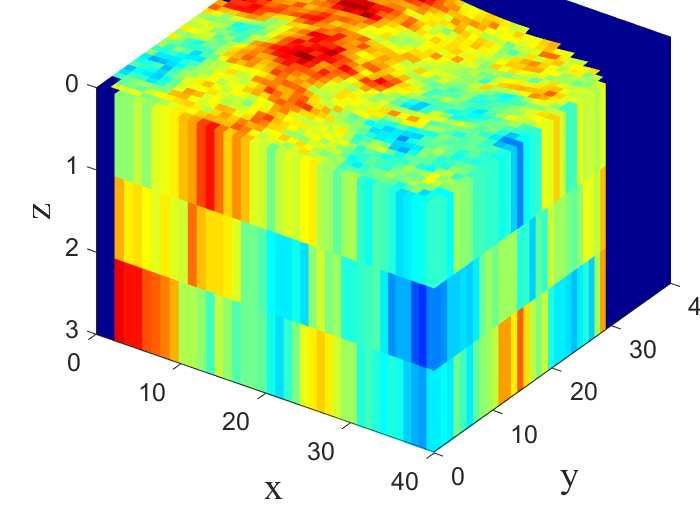
for three random training scenarios of the 2D and 3D models are shown in Fig.3 (a) (b) (c) and
Fig.3 (d) (e) (f), respectively. Note that other variables (such as the constraints, economics and
fluid properties) for these training scenarios are, in general, different.
The simulations in both cases are performed using Delft Advanced Research Terra Simulator
(DARTS) with operator-based linearization (Khait and Voskov 2017; Khait 2019). The simulator
has a python interface that allows for easy coupling with the deep reinforcement learning frame-
work. The light weight nature of the simulator makes it suitable for running millions of simulations
with minimal overhead. The overhead is significantly reduced due to the absence of redundant
input/output processing. In our implementation, the simulator was further extended to handle dy-
namic addition of wells between drilling stages.
The training process utilizes 151 CPU cores for the 2D case and 239 CPU cores for the 3D
case. The CPU cores are used to run the simulations in parallel. The training data generated are
then passed to 4 GPU cores used for training the deep neural network. The weighting factors for
the terms in the loss function are defined based on those proposed in He et al. (2021). Accordingly,
ckl , cv f and cent in Eq. 7 are set to 0.2, 0.1, 0.001. A linear learning rate decay schedule is used
for the gradient descent with an initial learning rate of 1e−3 and a final learning rate of 5e−6 (at
15 million training samples). It should be noted that each combination of at , st and rt generated inDRL for Constrained FDO 15
0.25
10 10 10
0.2
20 20 20
0.15
y
y
y
30 30 30
0.1
40 40 40 0.05
50 50 50
10 20 30 40 50 10 20 30 40 50 10 20 30 40 50
x x x
(a) (b) (c)
(d) (e) (f)
Fig. 3: Porosity fields for random training scenarios of the 2D and 3D models sampled from the
parameter distributions given in Table 1.
each drilling stage represents a single training sample. A mini-batch size of 256 and 5 epochs are
used for the gradient descent.
For the 2D case, we first compare the performance of the action parameterization used in our
previous work He et al. (2021), with the one proposed in this work. We then benchmark the per-
formance of the 2D artificial intelligence agent with well-pattern drilling agents. The 3D artificial
intelligence agent is also compared with the well-pattern drilling agents.
4.1 Case 1: Two-dimensional system
We now present results for the 2D case. Figure 4 shows the evolution of some performance in-
dicators for the training process in which the dual-action probability distribution is used. At each
of the training iteration, each of the 151 CPUs runs a maximum of two simulations. The set of
training data generated (used to train the agent in that specific iteration) are used to compute the
performance indicators reported. The training of the agent involves approximately two million sim-
ulations, which corresponds to approximately 7,100 equivalent simulations or training iterations.
From Fig. 4 (a), it is evident that the average NPV of the field development scenarios, in general,
increases as the training progresses. Starting from a random policy (randomly initiated weights
of the deep neural network) which results in negative average NPV, the average NPV increased
to more than $2 billion. The fluctuation in the average NPV is due to the fact that the ease of16 Y. Nasir, J. He, C. Hu, S. Tanaka, K. Wang, X. Wen
developing the various field development scenarios, which are randomly generated, varies from
iteration to another.
3000 0
Minim um NPV ($ Million)
Average NPV ($ Million)
− 2000
2000
− 4000
1000
− 6000
0
− 8000
− 1000 − 10000
0.0 0.5 1.0 1.5 2.0 0.0 0.5 1.0 1.5 2.0
Num ber of sim ulat ions (m illion) Num ber of sim ulat ions (m illion)
(a) Average NPV (b) Minimum NPV
2500 25000
Value funct ion loss
2000 20000
Tot al loss
1500 15000
1000 10000
500 5000
0 0
0.0 0.5 1.0 1.5 2.0 0.0 0.5 1.0 1.5 2.0
Num ber of sim ulat ions (m illion) Num ber of sim ulat ions (m illion)
(c) Total loss (d) Value function loss
8.0
7.5 0.05
Policy loss
7.0
Ent ropy
0.00
6.5
6.0 − 0.05
5.5
− 0.10
0.0 0.5 1.0 1.5 2.0 0.0 0.5 1.0 1.5 2.0
Num ber of sim ulat ions (m illion) Num ber of sim ulat ions (m illion)
(e) Entropy (f) Policy loss
Fig. 4: Evolution of training performance metrics for the dual-action probability distributions for
the 2D case.DRL for Constrained FDO 17
Figure 4 (b) shows the minimum NPV of the field development scenarios generated at each
iteration. Theoretically, the agent should have a minimum NPV of zero as it could choose not to
drill any well. However, it should be noted that during the generation of the training data, the action
to be taken is sampled from the action distribution of the policy. While this aids in exploring the
action space (the entropy loss also encourages exploration) and improves the training performance,
it also means the policy is not strictly followed during training. This leads to some fluctuation in the
minimum NPV in Fig. 4 (b), but overall the minimum NPV approaches zero. During the application
of the agent (after training), the action with the maximum probability is taken. Results for the case
in which the policy is followed strictly are presented later.
The PPO total loss, given in Eq. 7, is shown in Figure 4 (c). The loss, in general, decreases as the
optimization progresses. The value function loss, entropy and policy loss are shown in Fig. 4 (d),
(e), and (f), respectively. From the figures, we can see that the total loss is dominated by the
value function loss. From our limited experimentation, there was no noticeable advantage in the
reduction of the weighting factor for the value function loss. The entropy loss which indicates the
convergence of the policy can be seen to be decreasing. The policy loss, however, oscillates and
does not show any clear trend. This is a common behaviour in reinforcement learning because the
definition of the policy loss varies from one iteration to another.
Fig. 5: Evolution of the average NPV us-
ing the single-action probability distribu-
Average NPV ($ Million)
tion for the 2D case. 2000
1000
0
− 1000
0.0 0.5 1.0 1.5 2.0
Num ber of sim ulat ions (m illion)
We now compare the performance of the single-action probability distribution used in He et al.
(2021) with the dual-action probability distribution. Figure 5 shows the evolution of the average
NPV for the single-action probability distribution. In general, the average NPV increases as the
training progresses. However, when compared to Fig. 4 (a), the use of a single-action probability
distribution leads to a slow learning in the initial training phase. The result shown here is the
best found after several trials. Depending on the initial policy, the learning could be significantly
slower than the case shown here. This slow learning is mainly because the learning of the decision
not to drill a well is very slow since the action probability distribution is dominated by possible
drilling locations. This slow learning increases the computational cost of the training because the
timing of the simulation generally increases with number of wells. The timing for the first 100,000
simulations when the single-action probability distribution is used is 11.8 hours. This is in contrast
to 7.6 hours for the dual-action probability distribution case, leading to a computational cost saving
of approximately 4 hours for the initial 100,000 simulations.18 Y. Nasir, J. He, C. Hu, S. Tanaka, K. Wang, X. Wen
Fig. 6: Evolution of the average NPV for
the single and dual-action probability dis-
tributions.
As noted earlier, during training, there is an exploratory aspect to the agent’s policy and the field
development scenarios are randomly generated. For this reason, we generate 150 random field de-
scriptions, fluid properties, economics and constraints which are used for consistent comparison of
the training performance of the single and dual action distributions. Figure 6 shows the evolution of
the average NPV for the 150 field development scenarios. The agent after every 100 training itera-
tion is applied for the development of the 150 scenarios. Clearly, the use of dual-action probability
distribution outperforms the single-action probability distribution.
Once the AI agent is trained, it can be used to generate optimized field development plans for
any new scenarios within the range of applicability without additional simulations. Its extremely
low cost in optimization for new scenarios makes it distinctively different from the traditional
optimization methods, which for any new scenario would require hundreds or thousands of simu-
lations.
The performance of the best AI agent found using the dual-action probability distribution is
now compared to reference well-pattern agents. The best artificial intelligence agent is taken to
be the agent with the maximum average NPV of the 150 field development scenarios previously
considered. The reference well patterns considered include the 4-, 5-, 9- and 16-spot patterns which
are illustrated in Fig. 7. Note that these patterns are made up of only production wells and the wells
are equally spaced. Wells that fall in the inactive region (dark-blue region) of the reservoir are not
considered in the field development. For example, wells P3 and P9 in the 9-spot pattern (Fig. 7 (c))
and wells P4 and P16 in the 16-spot pattern (Fig. 7 (d)) are removed from the development plan.
Figure 8 (a), (b), (c), and (d) shows the performance of the artificial intelligence agent against
the 4-, 5-, 9- and 16-spot reference well patterns, respectively. In all four cases, the artificial intel-
ligence agent outperforms the reference well patterns in at least 96% of the 150 field development
scenarios considered.
Figure 8 (e) shows the comparison of the NPV obtained from the artificial intelligence agent
with the maximum NPV obtained from the four well-pattern agents for each of the 150 field devel-
opment scenarios. In this case, the artificial intelligent agent outperforms the maximum from all
well-pattern agents in approximately 92% of the field development scenarios. The minimum NPV
obtained by the artificial intelligence agent in the 150 field development scenarios is zero NPV.
For a significant proportion of these cases, the drilling of wells using the well-pattern agents leads
to negative NPV, while the AI agent simply recommended not to develop the field. The resultsDRL for Constrained FDO 19
0 0
10 0.15 10 0.15
P1 P3 P1 P3
20 20
0.10 P5 0.10
30 30
P2 P4 0.05 P2 P4 0.05
40 40
0 20 40 0 20 40
(a) 4-spot (b) 5-spot
0 0
P1 P4 P7 P1 P5 P9 P1 3
10 0.15 10 0.15
20 20 P2 P6 P1 0 P1 4
P2 P5 P8 0.10 0.10
30 30 P3 P7 P1 1 P1 5
0.05 0.05
40 P3 P6 P9 40
P4 P8 P1 2 P1 6
0 20 40 0 20 40
(c) 9-spot (d) 16-spot
Fig. 7: Illustration of the 4-, 5-, 9- and 16-spot well pattern with the background as the porosity
field of a specific test scenario.
demonstrate the ability of the artificial intelligence agent to identify unfavorable field development
scenarios. Although not considered in this work, various well spacing, well-pattern geometry, or
orientation, such as those discussed in well-pattern optimization (Onwunalu and Durlofsky 2011;
Nasir et al. 2021), could be used to further refine the performance of the artificial intelligence
agent.
The positioning of wells by the artificial intelligence agent for three random cases out of the
150 field development scenarios are shown in Fig. 9. These cases entails field development plans
with six, five, and nine production wells, in scenario 1, 2, and 3, respectively. All wells in the
three scenarios are drilled early. For example, in scenario 1, the six wells are drilled in the first six
drilling stages with well P1 drilled in the first drilling stage and P6 in the sixth drilling stage. The
wells are strategically placed in regions of the reservoir with high productivity (Fig. 9 (a) (d) (g))
and oil accumulation (Fig. 9 (b) (e) (h)). The pressure distributions for the scenarios are shown in
Fig. 9 (c) (f) (i). The wells are also properly spaced resulting in a good coverage of the producing
region.20 Y. Nasir, J. He, C. Hu, S. Tanaka, K. Wang, X. Wen
4.2 Case 2: Three-dimensional system
Results from the training of the agent for the 3D subsurface system is now presented. For the 3D
case, the wells are assumed to be always vertical and fully penetrate all layers of the reservoir in
this work. The procedures discussed in this work can, however, be readily extended to horizontal
wells with varying completion strategies. Compared to that of the 2D case, a larger neural network
(in terms of number of learnable parameters) is used to represent the policy for the 3D case. This
is because the size of the input channels to the agent is larger than that of the 2D case. The vertical
heterogeneity in the reservoir models is captured by including the transmissibility in the Z-direction
in the state representation.
Figure 10 shows the evolution of the performance indicators for the training process using the
dual-action probability distribution for the 3D case. The training entails approximately 2 million
simulations. From Fig. 10 (a) it can be seen that the average NPV generally increases as the training
progresses. This demonstrates the artificial intelligence agent can learn the field development logic
for the even more complicated three-dimensional system. Consistent with the behaviour of the
agent for the two-dimensional case when the dual-action probability distribution is used, we see a
rapid increase in average NPV during the initial phase of the training. As observed in the 2D case,
the total loss (Fig. 10 (c)), value function loss (Fig. 10 (d)), and entropy loss (Fig. 10 (e)) decrease
as the training progresses.
The performance of the best artificial intelligence agent is also compared with the four refer-
ence well-pattern agents for a set of random field development scenarios. The performance of the
artificial intelligence agent against the maximum NPV obtained from the four well-pattern agents
(same as those considered in the 2D case) is shown in Fig. 11. The artificial intelligence agent
outperforms the well-pattern agents in approximately 88% of the cases considered.
Figure 12 shows the well configurations proposed by the best AI agent for three random field
development scenarios. The field development plans involves eight, four and five production wells.
5 Concluding Remarks
In this work, we developed an AI agent for constrained field development optimization for two-
and three-dimensional subsurface two-phase flow models. The training of the agent utilizes the
concept of deep reinforcement learning where a feedback paradigm is used to continuously im-
prove the performance of the agent through experience. The experience includes the action or
decision taken by the agent, how this action affects the state of the environment (on which the ac-
tion is taken), and the corresponding reward which indicates the quality of the action. The training
efficiency is enhanced using a dual-action probability distribution parameterization and a convo-
lutional neural network architecture with shared layers for the policy and value functions of the
agent. After appropriate training, the agent instantaneously provides optimized field development
plan, which includes the number of wells to drill, their location, and drilling sequence for different
field development scenarios within a predefined range of applicability.
Example cases involving 2D and 3D subsurface systems are used to assess the performance
of the training procedure and the resulting artificial intelligence agent. The use of the dual-action
probability distribution shows clear advantage over the single-action probability distribution for
the training of the artificial intelligence agent. The trained artificial intelligence agents for the
2D and 3D case are shown to outperform four reference well-pattern agents. For the 2D case,You can also read