ROBUST REINFORCEMENT LEARNING USING ADVERSARIAL POPULATIONS
←
→
Page content transcription
If your browser does not render page correctly, please read the page content below
Under review as a conference paper at ICLR 2021

ROBUST R EINFORCEMENT L EARNING
USING A DVERSARIAL P OPULATIONS

 Anonymous authors
 Paper under double-blind review

                                           A BSTRACT
         Reinforcement Learning (RL) is an effective tool for controller design but can
         struggle with issues of robustness, failing catastrophically when the underlying
         system dynamics are perturbed. The Robust RL formulation tackles this by adding
         worst-case adversarial noise to the dynamics and constructing the noise distribution
         as the solution to a zero-sum minimax game. However, existing work on learning
         solutions to the Robust RL formulation has primarily focused on training a single
         RL agent against a single adversary. In this work, we demonstrate that using a
         single adversary does not consistently yield robustness to dynamics variations
         under standard parametrizations of the adversary; the resulting policy is highly
         exploitable by new adversaries. We propose a population-based augmentation to the
         Robust RL formulation in which we randomly initialize a population of adversaries
         and sample from the population uniformly during training. We empirically validate
         across robotics benchmarks that the use of an adversarial population results in a
         less exploitable, more robust policy. Finally, we demonstrate that this approach
         provides comparable robustness and generalization as domain randomization on
         these benchmarks while avoiding a ubiquitous domain randomization failure mode.

1   I NTRODUCTION
Developing controllers that work effectively across a wide range of potential deployment environments
is one of the core challenges in engineering. The complexity of the physical world means that the
models used to design controllers are often inaccurate. Optimization based control design approaches,
such as reinforcement learning (RL), have no notion of model inaccuracy and can lead to controllers
that fail catastrophically under mismatch. In this work, we aim to demonstrate an effective method for
training reinforcement learning policies that are robust to model inaccuracy by designing controllers
that are effective in the presence of worst-case adversarial noise in the dynamics.
An easily automated approach to inducing robustness is to formulate the problem as a zero-sum
game and learn an adversary that perturbs the transition dynamics (Tessler et al., 2019; Kamalaruban
et al., 2020; Pinto et al., 2017). If a global Nash equilibrium of this problem is found, then that
equilibrium provides a lower bound on the performance of the policy under some bounded set of
perturbations. Besides the benefit of removing user design once the perturbation mechanism is
specified, this approach is maximally conservative, which is useful for safety critical applications.
However, the literature on learning an adversary predominantly uses a single, stochastic adversary.
This raises a puzzling question: the zero-sum game does not necessarily have any pure Nash equilibria
(see Appendix C in Tessler et al. (2019)) but the existing robust RL literature mostly appears to
attempt to solve for pure Nash equilibria. That is, the most general form of the minimax problem
searches over distributions of adversary and agent policies, however, this problem is approximated
in the literature by a search for a single agent-adversary pair. We contend that this reduction to
a single adversary approach can sometimes fail to result in improved robustness under standard
parametrizations of the adversary policy.
The following example provides some intuition for why using a single adversary can decrease
robustness. Consider a robot trying to learn to walk east-wards while an adversary outputs a force
representing wind coming from the north or the south. For a fixed, deterministic adversary the agent
knows that the wind will come from either south or north and can simply apply a counteracting force
at each state. Once the adversary is removed, the robot will still apply the compensatory forces and

                                                  1
Under review as a conference paper at ICLR 2021

possibly become unstable. Stochastic Gaussian policies (ubiquitous in continuous control) offer
little improvement: they cannot represent multi-modal perturbations. Under these standard policy
parametrizations, we cannot use an adversary to endow the agent with a prior that a strong wind could
persistently blow either north or south. This leaves the agent exploitable to this class of perturbations.
The use of a single adversary in the robustness literature is in contrast to the multi-player game
literature. In multi-player games, large sets of adversaries are used to ensure that an agent cannot
easily be exploited (Vinyals et al., 2019; Czarnecki et al., 2020; Brown & Sandholm, 2019). Drawing
inspiration from this literature, we introduce RAP (Robustness via Adversary Populations): a
randomly initialized population of adversaries that we sample from at each rollout and train alongside
the agent. Returning to our example of a robot perturbed by wind, if the robot learns to cancel the
north wind effectively, then that opens a niche for an adversary to exploit by applying forces in
another direction. With a population, we can endow the robot with the prior that a strong wind could
come from either direction and that it must walk carefully to avoid being toppled over.
Our contributions are as follows:

      • Using a set of continuous robotics control tasks, we provide evidence that a single adversary
        does not have a consistent positive impact on the robustness of an RL policy while the use
        of an adversary population provides improved robustness across all considered examples.
      • We investigate the source of the robustness and show that the single adversary policy
        is exploitable by new adversaries whereas policies trained with RAP are robust to new
        adversaries.
      • We demonstrate that adversary populations provide comparable robustness to domain
        randomization while avoiding potential failure modes of domain randomization.

2    R ELATED W ORK
This work builds upon robust control (Zhou & Doyle, 1998), a branch of control theory focused
on finding optimal controllers under worst-case perturbations of the system dynamics. The Robust
Markov Decision Process (R-MDP) formulation extends this worst-case model uncertainty to uncer-
tainty sets on the transition dynamics of an MDP and demonstrates that computationally tractable
solutions exist for small, tabular MDPs (Nilim & El Ghaoui, 2005; Lim et al., 2013). For larger
or continuous MDPs, one successful approach has been to use function approximation to compute
approximate solutions to the R-MDP problem (Tamar et al., 2014).
One prominent variant of the R-MDP literature is to interpret the perturbations as an adversary and
attempt to learn the distribution of the perturbation under a minimax objective. Two variants of this
idea that tie in closely to our work are Robust Adversarial Reinforcement Learning (RARL)(Pinto
et al., 2017) and Noisy Robust Markov Decision Processes (NR-MDP) (Tessler et al., 2019) which
differ in how they parametrize the adversaries: RARL picks out specific robot joints that the adversary
acts on while NR-MDP adds the adversary action to the agent action. Both of these works attempt to
find an equilibrium of the minimax objective using a single adversary; in contrast our work uses a
large set of adversaries and shows improved robustness relative to a single adversary.
A strong alternative to the minimax objective, domain randomization, asks a designer to explicitly
define a distribution over environments that the agent should be robust to. For example, (Peng et al.,
2018) varies simulator parameters to train a robot to robustly push a puck to a target location in the
real world; (Antonova et al., 2017) adds noise to friction and actions to transfer an object pivoting
policy directly from simulation to a Baxter robot. Additionally, domain randomization has been
successfully used to build accurate object detectors solely from simulated data (Tobin et al., 2017)
and to zero-shot transfer a quadcopter flight policy from simulation (Sadeghi & Levine, 2016).
The use of population based training is a standard technique in multi-agent settings. Alphastar, the
grandmaster-level Starcraft bot, uses a population of "exploiter" agents that fine-tune against the
bot to prevent it from developing exploitable strategies (Vinyals et al., 2019). (Czarnecki et al.,
2020) establishes a set of sufficient geometric conditions on games under which the use of multiple
adversaries will ensure gradual improvement in the strength of the agent policy. They empirically
demonstrate that learning in games can often fail to converge without populations. Finally, Active
Domain Randomization (Mehta et al., 2019) is a very close approach to ours, as they use a population

                                                    2
Under review as a conference paper at ICLR 2021

of adversaries to select domain randomization parameters whereas we use a population of adversaries
to directly perturb the agent actions. However, they explicitly induce diversity using a repulsive term
and use a discriminator to generate the reward.

3     BACKGROUND

In this work we use the framework of a multi-agent, finite-horizon, discounted, Markov Decision
Process (MDP) (Puterman, 1990) defined by a tuple hAagent × Aadversary , S, T , r, γi. Here Aagent is
the set of actions for the agent, Aadversary is the set of actions for the adversary, S is a set of states,
T : Aagent × Aadversary × S → ∆(S) is a transition function, r : Aagent × Aadversary × S → R is
a reward function and γ is a discount factor. S is shared between the adversaries as they share
a state-space with the agent. The goal for a given MDP is to find a policy  hP πθ parametrized     i by θ
                                                                    θ          T     t
that maximizes the expected cumulative discounted reward J = E                 t=0 γ r(st , at )|πθ . The
conditional in this expression is a short-hand to indicate that the actions in the MDP are sampled via
at ∼ πθ (st , at−1 ). We denote the agent policy parametrized by weights θ as πθ and the policy of
adversary i as π̄φi . Actions sampled from the adversary policy π̄φi will be written as āit . We use ξ to
denote the parametrization of the system dynamics (e.g. different values of friction, mass, wind, etc.)
and the system dynamics for a given state and action as st+1 ∼ fξ (st , at ).

3.1     BASELINES

Here we outline prior work and the approaches that will be compared with RAP. Our baselines consist
of a single adversary and domain randomization.

3.1.1    S INGLE M INIMAX A DVERSARY

Our adversary formulation uses the Noisy Action Robust MDP (Tessler et al., 2019) in which the
adversary adds its actions onto the agent actions. The objective is

                                        " T                                      #
                                         X
                                                 t
                                max E          γ r(st , at + αa¯t )|πθ , π̄φ
                                 θ
                                         t=0
                                        " T                                      #                     (1)
                                         X
                                min E          γ t r(st , at + αa¯t )|πθ , π̄φ
                                 φ
                                         t=0

where α is a hyperparameter controlling the adversary strength. This is a game in which the adversary
and agent play simultaneously. We note an important restriction inherent to this adversarial model.
Since the adversary is only able to attack the agent through the actions, there is a restricted class of
dynamical systems that it can represent; this set of dynamical systems may not necessarily align with
the set of dynamical systems that the agent may be tested in. This is a restriction caused by the choice
of adversarial perturbation and could be alleviated by using different adversarial parametrizations e.g.
perturbing the transition function directly.

3.1.2    DYNAMICS R ANDOMIZATION

Domain randomization is the setting in which the user specifies a set of environments which the agent
should be robust to. This allows the user to directly encode knowledge about the likely deviations
between training and testing domains. For example, the user may believe that friction is hard to
measure precisely and wants to ensure that their agent is robust to variations in friction; they then
specify that the agent will be trained with a wide range of possible friction values. We use ξ to
denote some vector that parametrizes the set of training environments (e.g. friction, masses, system
dynamics, etc.). We denote the domain over which ξ is drawn from as Ξ and use P (Ξ) to denote

                                                       3
Under review as a conference paper at ICLR 2021

some probability distribution over ξ. The domain randomization objective is

                                        "                                  " T                              ##
                                                                            X
                                                                                     t
                        max Eξ∼P(Ξ) Est+1 ∼fξ (st ,at )                             γ r(st , at )|πθ
                          θ
                                                                              t=0                                  (2)
                                                st+1 ∼ fξ (st , at )
                                                   at ∼ πθ (st )

Here the goal is to find an agent that performs well on average across the distribution of training
environment. Most commonly, and in this work, the parameters ξ are sampled uniformly over Ξ.

4    RAP: ROBUSTNESS VIA A DVERSARY P OPULATIONS

RAP extends the minimax objective with a population based approach. Instead of a single adversary,
at each rollout we will sample uniformly from a population of adversaries. By using a population,
the agent is forced to be robust to a wide variety of potential perturbations rather than a single
perturbation. If the agent begins to overfit to any one adversary, this opens up a potential niche for
another adversary to exploit. For problems with only one failure mode, we expect the adversaries to
all come out identical to the minimax adversary, but as the number of failure modes increases the
adversaries should begin to diversify to exploit the agent. To induce this diversity, we will rely on
randomness in the gradient estimates and randomness in the initializations of the adversary networks
rather than any explicit term that induces diversity.
Denoting π̄φi as the i-th adversary and i ∼ U (1, n) as the discrete uniform distribution defined on 1
through n, the objective becomes

                                                    "   T
                                                                                                        #
                                                        X
                                                                  t
                              max Ei∼U (1,n)                  γ       r(st , at , αāit )|πθ ,   π̄φi
                               θ
                                                        t=0
                                      " T                                                  #
                                       X                                                                           (3)
                                                t
                              min E         γ       r(st , at , αāit )|πθ ,        π̄φi       ∀i = 1, . . . , n
                              φi
                                      t=0
                                        st+1 ∼ f (st , at + αa¯t )

For a single adversary, this is equivalent to the minimax adversary described in Sec. 3.1.1. This is a
game in which the adversary and agent play simultaneously.
We will optimize this objective by converting the problem into the equivalent zero-sum game. At the
start of each rollout, we will sample an adversary index from the uniform distribution and collect
a trajectory using the agent and the selected adversary. For notational simplicity, we assume the
trajectory is of length T and that adversary i will participate in Ji total trajectories while, since
the agent participates in every rollout, the agent will receive J total trajectories. We denote the
j-th collected trajectory for the agent as τj = (s0 , a0 , r0 , s1 ) × · · · × (sM , aM , rM , sM +1 ) and
the associated trajectory for adversary i as τji = (s0 , a0 , −r0 , s1 ) × · · · × (sM , aM , −rM , sM ).
Note that the adversary reward is simply the negative of the agent reward. We will use Proximal
Policy Optimization (Schulman et al., 2017) (PPO) to update our policies. We caution that we have
                                                        i
overloaded notation slightly here and for adversary i, τj=1:J  i
                                                                 refers only to the trajectories in which
the adversary was selected: adversaries will only be updated using trajectories where they were active.

                                                                  4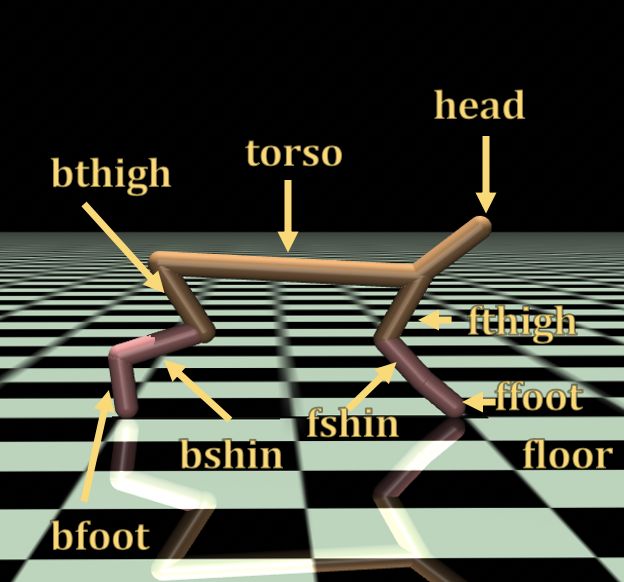
Under review as a conference paper at ICLR 2021

At the end of a training iteration, we update all our policies using gradient descent. The algorithm is
summarized below:
Algorithm 1: Robustness via Adversary Populations
Initialize θ, φ1 · · · φn using Xavier initialization (Glorot & Bengio, 2010);
while not converged do
     for rollout j=1...J do
         sample adversary i ∼ U (1, n);
         run policies πθ , π̄φi in environment until termination;
         collect trajectories τj , τji
     end
     update θ, φ1 · · · φn using PPO (Schulman et al., 2017) and trajectories τj for θ and τji for each
      φi ;
end

5     E XPERIMENTS
In this section we present experiments on continuous control tasks from the OpenAI Gym Suite
(Brockman et al., 2016; Todorov et al., 2012). We compare with the existing literature and evaluate
the efficacy of a population of learned adversaries across a wide range of state and action space sizes.
We investigate the following hypotheses:

      H1. Agents are more likely to overfit to a single adversary than a population of adversaries,
          leaving them less robust on in-distribution tasks.
      H2. Agents trained against a population of adversaries will generalize better, leading to improved
          performance on out-of-distribution tasks.

In-distribution tasks refer to the agent playing against perturbations that are in the training distribution:
adversaries that add their actions onto the agent. However, the particular form of the adversary and
their restricted perturbation magnitude means that there are many dynamical systems that they
cannot represent (for example, significant variations of joint mass and friction). These tasks are
denoted as out-of-distribution tasks. All of the tasks in the test set described in Sec. 5.1 are likely
out-of-distribution tasks.

5.1     E XPERIMENTAL S ETUP AND H YPERPARAMETER S ELECTION

While we provide exact details of the hyperparameters in the Appendix, adversarial settings require
additional complexity in hyperparameter selection. In the standard RL procedure, optimal hyperpa-
rameters are selected on the basis of maximum expected cumulative reward. However, if an agent
playing against an adversary achieves a large cumulative reward, it is possible that the agent was
simply playing against a weak adversary. Conversely, a low score does not necessarily indicate a
strong adversary nor robustness: it could simply mean that we trained a weak agent.
To address this, we adopt a version of the train-validate-test split from supervised learning. We use
the mean policy performance on a suite of validation tasks to select the hyperparameters, then we
train the policy across ten seeds and report the resultant mean and standard deviation over twenty
trajectories. Finally, we evaluate the seeds on a holdout test set of eight additional model-mismatch
tasks. These tasks vary significantly in difficulty; for visual clarity we report the average across tasks
in this paper and report the full breakdown across tasks in the Appendix.
We experiment with the Hopper, Ant, and Half Cheetah continuous control environments used in
the original RARL paper Pinto et al. (2017); these are shown in Fig. 1. To generate the validation
model mismatch, we pre-define ranges of mass and friction coefficients as follows: for Hopper, mass
∈ [0.7, 1.3] and friction ∈ [0.7, 1.3]; Half Cheetah and Ant, mass ∈ [0.5, 1.5] and friction ∈ [0.1, 0.9].
We scale the friction of every Mujoco geom and the mass of the torso with the same (respective)
coefficients. We compare the robustness of agents trained via RAP against: 1) agents trained against
a single adversary in a zero-sum game, 2) oracle agents trained using domain randomization, and 3)
an agent trained only using PPO and no perturbation mechanism. To train the domain randomization

                                                     5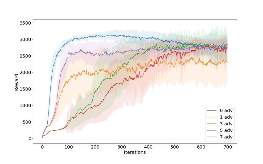
Under review as a conference paper at ICLR 2021

Figure 1: From left to right, the Hopper, Half-Cheetah, and Ant environments we use to test our
algorithm.

oracle, at each rollout we uniformly sample a friction and mass coefficient from the validation
set ranges. We then scale the friction of all geoms and the mass of the torso by their respective
coefficients; this constitutes directly training on the validation set. To generate the test set of model
mismatch, we take both the highest and lowest friction coefficients from the validation range and
apply them to different combinations of individual geoms. For the exact selected combinations,
please refer to the Appendix.
As further validation of the benefits of RAP, we include an additional set of experiments on a
continuous control task, a gridworld maze search task, and a Bernoulli Bandit task in Appendix
Sec. F. Finally, we note that both our agent and adversary networks are two layer-neural networks
with 64 hidden units in each layer and a tanh nonlinearity.

6   R ESULTS

H1. In-Distribution Tasks: Analysis of Overfitting
A globally minimax optimal adversary should be unexploitable and perform equally well against
any adversary of equal strength. We investigate the optimality of our policy by asking whether the
minimax agent is robust to swaps of adversaries from different training runs, i.e. different seeds.
Fig. 2 shows the result of these swaps for the one adversary and three adversary case. The diagonal
corresponds to playing against the adversaries the agent was trained with while every other square
corresponds to playing against adversaries from a different seed. To simplify presentation, in the
three adversary case, each square is the average performance against all the adversaries from that
seed. We observe that the agent trained against three adversaries (top row right) is robust under swaps
while the single adversary case is not (top row left). The agent trained against a single adversary is
highly exploitable, as can be seen by its extremely sub-par performance against an adversary from
any other seed. Since the adversaries off-diagonal are feasible adversaries, this suggests that we have
found a poor local optimum of the objective.
In contrast, the three adversary case is generally robust regardless of which adversary it plays against,
suggesting that the use of additional adversaries has made the agent more robust. One possible
hypothesis for why this could be occurring is that the adversaries in the "3 adversary" case are
somehow weaker than the adversaries in the "1 adversary" case. The middle row of the figure shows
that it is not the case that the improved performance of the agent playing against the three adversaries
is due to some weakness of the adversaries. If anything, the adversaries from the three adversary case
are stronger as the agent trained against 1 adversary does extremely poorly playing against the three
adversaries (left) whereas the agent trained against three adversaries still performs well when playing
against the adversaries from the single-adversary runs. Finally, the bottom row investigates how an
agent trained with domain randomization fairs against adversaries from either training regimes. In
neither case is the domain randomization agent robust on these tasks.
H2. Out-of-Distribution Tasks: Robustness and Generalization of Population Training
Here we present the results from the validation and holdout test sets described in Section 5.1. We
compare the performance of training with adversary populations of size three and five against vanilla
PPO, the domain randomization oracle, and the single minimax adversary. We refer to domain
randomization as an oracle as it is trained directly on the test distribution.
Fig.6 shows the average reward (the average of ten seeds across the validation or test sets respectively)
for each environment. Table 1 gives the corresponding numerical values and the percent change of
each policy from the baseline. Standard deviations are omitted on the test set due to wide variation
in task difficulty; the individual tests that we aggregate here are reported in the Appendix with

                                                   6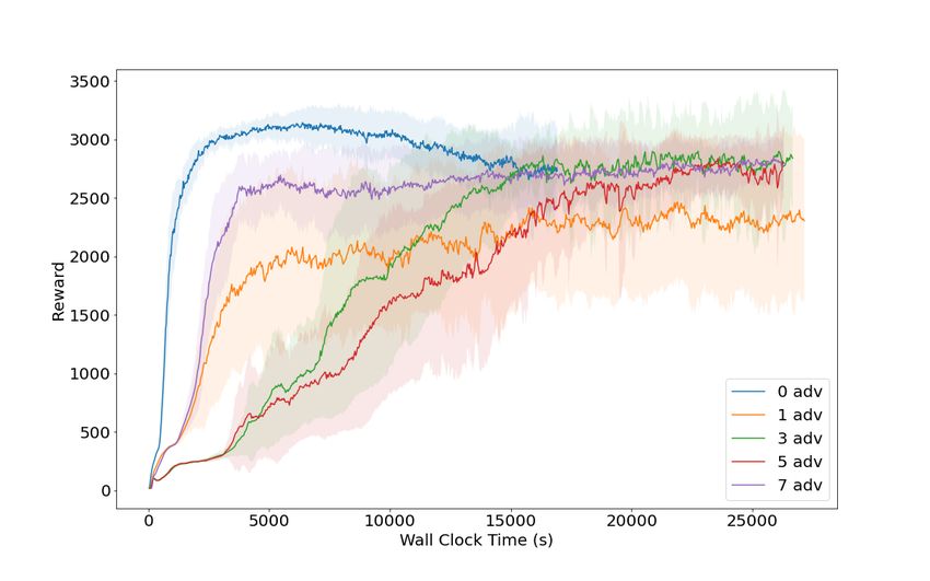
Under review as a conference paper at ICLR 2021

Figure 2: Top row: Average cumulative reward under swaps for one adversary training (left) and
three-adversary training (right). Each square corresponds to 20 trials. In the three adversary case,
each square is the average performance against the adversaries from that seed. Middle row: (Left)
Playing the agent trained against 1 adversary against the adversaries from the three adversary case.
(Right) Playing the agent trained against 3 adversaries against the adversaries from the one adversary
case. Bottom row: (Left) Playing the DR agent against the adversaries from the three adversary case.
(Right) Playing the DR agent against the adversaries from the one adversary case.

appropriate error bars. In all environments we achieve a higher reward across both the validation and
holdout test set using RAP of size three and/or five when compared to the single minimax adversary
case. These results from testing on new environments with altered dynamics supports hypothesis
H2. that training with a population of adversaries leads to more robust policies than training with a
single adversary in out-of-distribution tasks. Furthermore, while the performance is only comparable
with the domain randomization oracle, the adversarial approach does not require prior engineering
of appropriate randomizations. Furthermore, despite domain randomization being trained directly
on these out-of-distribution tasks, domain randomization can have serious failure modes of domain
randomization due to its formulation. A detailed analysis of this can be found in Appendix E.
For a more detailed comparison of robustness across the validation set, Fig. 4 shows heatmaps of the
performance across all the mass, friction coefficient combinations. Here we highlight the heatmaps
for Hopper and Half Cheetah for vanilla PPO, domain randomization oracle, single adversary, and
best adversary population size. Additional heatmaps for other adversary population sizes and the Ant
environment can be found in the Appendix. Note that Fig. 4 is an example of a case where a single
adversary has negligible effect on or slightly reduces the performance of the resultant policy on the

                                                  7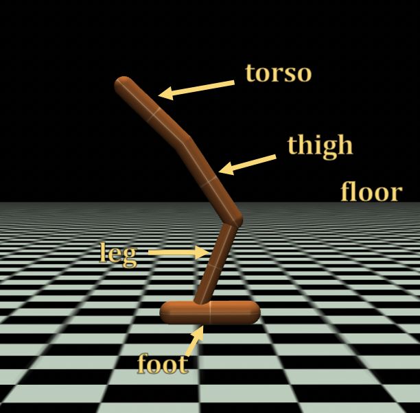
Under review as a conference paper at ICLR 2021

Figure 3: Average reward for Ant, Hopper, and Cheetah environments across ten seeds and across the
validation set (top row) and across the holdout test set (bottom row). We compare vanilla PPO, the
domain randomization oracle, and the minimax adversary against RAP of size three and five. Bars
represent the mean and the arms represent the std. deviation. Both are computed over 20 rollouts for
each test-set sample. The std. deviation for the test set are not reported here for visual clarity due to
the large variation in holdout test difficulty.

                              Validation                                        Test
      Ant       0 Adv      DR  1 Adv 3 Adv          5 Adv    0 Adv     DR     1 Adv    3 Adv    5 Adv
    Mean Rew.   6336      6743 6349      6432       6438     2908     3613    3206     3272     3203
    % Change               6.4   0.2      1.5        1.6              24.3     10.2     12.5     10.2
                              Validation                                        Test
     Hopper     0 Adv     DR   1 Adv 3 Adv         5 Adv     0 Adv     DR     1 Adv    3 Adv    5 Adv
    Mean Rew.   1182     2662  1094      2039      2021       472     1636     913     1598     1565
    % Change             125    -7.4     72.6        71                246     93.4     238      231
                              Validation                                        Test
     Cheetah    0 Adv     DR   1 Adv 3 Adv          5 Adv    0 Adv     DR     1 Adv    3 Adv    5 Adv
    Mean Rew.   5659     3864  5593      5912       6323     5592     3656    5664     6046     6406
    % Change              -32   -1.2      4.5        11.7              -35      1.3     8.1      14.6

Table 1: Average reward and % change from vanilla PPO (0 Adv) for Ant, Hopper, and Cheetah
environments across ten seeds and across the validation (left) or holdout test set (right). Across all
environments, we see consistently higher robustness using RAP than the minimax adversary. Most
robust adversarial approach is bolded as domain randomization is an oracle and outside the class of
perturbations that our adversaries can construct, and best result overall is italicized.

validation set. This supports our hypothesis that a single adversary can actually lower the robustness
of an agent.

7     C ONCLUSIONS AND F UTURE W ORK

In this work we demonstrate that the use of a single adversary to approximate the solution to a
minimax problem does not consistently lead to improved robustness. We propose a solution through
the use of multiple adversaries (RAP), and demonstrate that this provides robustness across a variety
of robotics benchmarks. We also compare RAP with domain randomization and demonstrate that
while DR can lead to a more robust policy, it requires careful parametrization of the domain we
sample from to ensure robustness. RAP does not require this tuning, allowing for use in domains
where appropriate tuning requires extensive prior knowledge or expertise.
There are several open questions stemming from this work. While we empirically demonstrate the
effects of RAP, we do not have a compelling theoretical understanding of why multiple adversaries
are helping. Perhaps RAP helps approximate a mixed Nash equilibrium as discussed in Sec. 1 or

                                                   8
Under review as a conference paper at ICLR 2021
Figure 4: Average reward across ten seeds on each validation set parametrization – friction coefficient
on the x-axis and mass coefficient on the y-axis. DR refers to domain randomization and X Adv is an
agent trained against X adversaries. Top row is Hopper and bottom row is Half Cheetah.
perhaps population based training increases the likelihood that one of the adversaries is strong?
Would the benefits of RAP disappear if a single adversary had the ability to represent mixed Nash?
There are some extensions of this work that we would like to pursue. We have looked at the robustness
of our approach in simulated settings; future work will examine whether this robustness transfers to
real-world settings. Additionally, our agents are currently memory-less and therefore cannot perform
adversary identification; perhaps memory leads to a system-identification procedure that improves
transfer performance. Our adversaries can also be viewed as forming a task distribution, allowing
them to be used in continual learning approaches like MAML (Nagabandi et al., 2018) where domain
randomization is frequently used to construct task distributions.
9Under review as a conference paper at ICLR 2021
R EFERENCES
Rika Antonova, Silvia Cruciani, Christian Smith, and Danica Kragic. Reinforcement learning for
pivoting task. arXiv preprint arXiv:1703.00472, 2017.
Greg Brockman, Vicki Cheung, Ludwig Pettersson, Jonas Schneider, John Schulman, Jie Tang, and
Wojciech Zaremba. Openai gym, 2016.
Noam Brown and Tuomas Sandholm. Superhuman ai for multiplayer poker. Science, 365(6456):
885–890, 2019.
Wojciech Marian Czarnecki, Gauthier Gidel, Brendan Tracey, Karl Tuyls, Shayegan Omidshafiei,
David Balduzzi, and Max Jaderberg. Real world games look like spinning tops. arXiv preprint
arXiv:2004.09468, 2020.
Xavier Glorot and Yoshua Bengio. Understanding the difficulty of training deep feedforward neural
networks. In Proceedings of the thirteenth international conference on artificial intelligence and
statistics, pp. 249–256, 2010.
Parameswaran Kamalaruban, Yu-Ting Huang, Ya-Ping Hsieh, Paul Rolland, Cheng Shi, and Volkan
Cevher. Robust reinforcement learning via adversarial training with langevin dynamics. arXiv
preprint arXiv:2002.06063, 2020.
Eric Liang, Richard Liaw, Philipp Moritz, Robert Nishihara, Roy Fox, Ken Goldberg, Joseph E
Gonzalez, Michael I Jordan, and Ion Stoica. Rllib: Abstractions for distributed reinforcement
learning. arXiv preprint arXiv:1712.09381, 2017.
Shiau Hong Lim, Huan Xu, and Shie Mannor. Reinforcement learning in robust markov decision
processes. In Advances in Neural Information Processing Systems, pp. 701–709, 2013.
Bhairav Mehta, Manfred Diaz, Florian Golemo, Christopher J Pal, and Liam Paull. Active domain
randomization. arXiv preprint arXiv:1904.04762, 2019.
Anusha Nagabandi, Chelsea Finn, and Sergey Levine. Deep online learning via meta-learning:
Continual adaptation for model-based rl. arXiv preprint arXiv:1812.07671, 2018.
Arnab Nilim and Laurent El Ghaoui. Robust control of markov decision processes with uncertain
transition matrices. Operations Research, 53(5):780–798, 2005.
Xue Bin Peng, Marcin Andrychowicz, Wojciech Zaremba, and Pieter Abbeel. Sim-to-real transfer of
robotic control with dynamics randomization. In 2018 IEEE international conference on robotics
and automation (ICRA), pp. 1–8. IEEE, 2018.
Lerrel Pinto, James Davidson, Rahul Sukthankar, and Abhinav Gupta. Robust adversarial reinforce-
ment learning. In Proceedings of the 34th International Conference on Machine Learning-Volume
70, pp. 2817–2826. JMLR. org, 2017.
Martin L Puterman. Markov decision processes. Handbooks in operations research and management
science, 2:331–434, 1990.
Aravind Rajeswaran, Sarvjeet Ghotra, Balaraman Ravindran, and Sergey Levine. Epopt: Learning
robust neural network policies using model ensembles. arXiv preprint arXiv:1610.01283, 2016.
Fereshteh Sadeghi and Sergey Levine. Cad2rl: Real single-image flight without a single real image.
arXiv preprint arXiv:1611.04201, 2016.
John Schulman, Filip Wolski, Prafulla Dhariwal, Alec Radford, and Oleg Klimov. Proximal policy
optimization algorithms. arXiv preprint arXiv:1707.06347, 2017.
Aviv Tamar, Shie Mannor, and Huan Xu. Scaling up robust mdps using function approximation. In
International Conference on Machine Learning, pp. 181–189, 2014.
Yuval Tassa, Saran Tunyasuvunakool, Alistair Muldal, Yotam Doron, Siqi Liu, Steven Bohez, Josh
Merel, Tom Erez, Timothy Lillicrap, and Nicolas Heess. dm_control: Software and tasks for
continuous control. arXiv preprint arXiv:2006.12983, 2020.
10Under review as a conference paper at ICLR 2021
Chen Tessler, Yonathan Efroni, and Shie Mannor. Action robust reinforcement learning and applica-
tions in continuous control. arXiv preprint arXiv:1901.09184, 2019.
Josh Tobin, Rachel Fong, Alex Ray, Jonas Schneider, Wojciech Zaremba, and Pieter Abbeel. Domain
randomization for transferring deep neural networks from simulation to the real world. In 2017
IEEE/RSJ International Conference on Intelligent Robots and Systems (IROS), pp. 23–30. IEEE,
2017.
Emanuel Todorov, Tom Erez, and Yuval Tassa. Mujoco: A physics engine for model-based control.
In 2012 IEEE/RSJ International Conference on Intelligent Robots and Systems, pp. 5026–5033.
IEEE, 2012.
Oriol Vinyals, Igor Babuschkin, Wojciech M Czarnecki, Michaël Mathieu, Andrew Dudzik, Junyoung
Chung, David H Choi, Richard Powell, Timo Ewalds, Petko Georgiev, et al. Grandmaster level in
starcraft ii using multi-agent reinforcement learning. Nature, 575(7782):350–354, 2019.
Kemin Zhou and John Comstock Doyle. Essentials of robust control, volume 104. Prentice hall
Upper Saddle River, NJ, 1998.
A F ULL D ESCRIPTION OF THE C ONTINUOUS C ONTROL MDP S
We use the Mujoco ant, cheetah, and hopper environments as a test of the efficacy of our strategy
versus the 0 adversary, 1 adversary, and domain randomization baselines. We use the Noisy Action
Robust MDP formulation Tessler et al. (2019) for our adversary parametrization. If the normal system
dynamics are
sk+1 = sk + f (sk , ak )∆t
the system dynamics under the adversary are
sk+1 = sk + f (sk , ak + aadv
k )∆t
where aadv
k is the adversary action at time k.
The notion here is that the adversary action is passed through the dynamics function and represents
some additional set of dynamics. It is standard to clip actions within some boundary but for the above
reason, we clip the agent and adversary actions separately. Otherwise, an agent would be able to limit
the effect of the adversary by always taking actions at the bounds of its clipping range. The agent is
clipped between [−1, 1] in the Hopper environment and the adversary is clipped between [−.25, .25].
The MDP through which we train the agent policy is characterized by the following states, actions,
and rewards:
• sagent
t = [ot , at ] where ot is an observation returned by the environment, and at is the action
taken by the agent.
• We use the standard rewards provided by the OpenAI Gym Mujoco environments at https:
//github.com/openai/gym/tree/master/gym/envs/mujoco. For the exact
functions, please refer to the code at ANONYMIZED.
n
• aagent
t ∈ [amin , amax ] .
The MDP for adversary i is the following:
• st = sagent
t . The adversary sees the same states as the agent.
• The adversary reward is the negative of the agent reward.
adv adv n
• aadv
t ∈ amin , amax .
For our domain randomization Hopper baseline, we use the following randomization: at each
rollout, we scale the friction of all joints by a single value uniformly sampled from [0.7, 1.3]. We
also randomly scale the mass of the ’torso’ link by a single value sampled from [0.7, 1.3]. For
Half-Cheetah and Ant the range for friction is [0.1, 0.9] and for mass the range is [0.5, 1.5].
11Under review as a conference paper at ICLR 2021
Figure 5: Average reward for Hopper across varying adversary number.
B I NCREASING A DVERSARY P OOL S IZE
We investigate whether RAP is robust to adversary number as this would be a useful property to
minimize hyperparameter search. Here we hypothesize that while having more adversaries can
represent a wider range of dynamics to learn to be robust to, we expect there to be diminishing
returns due to the decreased batch size that each adversary receives (total number of environment
steps is held constant across all training variations). We expect decreasing batch size to lead to worse
agent policies since the batch will contain under-trained adversary policies. We cap the number of
adversaries at eleven as our machines ran out of memory at this value. We run ten seeds for every
adversary value and Fig. 5 shows the results for Hopper. Agent robustness on the test set increases
monotonically up to three adversaries and roughly begins to decrease after that point. This suggests
that a trade-off between adversary number and performance exists although we do not definitively
show that diminishing batch sizes is the source of this trade-off. However, we observe in Fig. 6 that
both three and five adversaries perform well across all studied Mujoco domains.
Figure 6: Average reward for Ant, Hopper, and Cheetah environments across ten seeds and across the
validation set (top row) and across the holdout test set (bottom row). We compare vanilla PPO, the
domain randomization oracle, and the minimax adversary against RAP of size three and five. Bars
represent the mean and the arms represent the std. deviation. Both are computed over 20 rollouts for
each test-set sample. The std. deviation for the test set are not reported here for visual clarity due to
the large variation in holdout test difficulty.
C H OLDOUT T ESTS
In this section we describe in detail all of the holdout tests used.
12Under review as a conference paper at ICLR 2021
Figure 7: Labelled Body Segments of Hopper
Table 2: Hopper Holdout Test Descriptions
Test Body with Friction Coeff 1.3 Body with Friction Coeff 0.7
A Torso, Leg Floor, Thigh, Foot
B Floor, Thigh Torso, Leg, Foot
C Foot, Leg Floor, Torso, Thigh
D Torso, Thigh, Floor Foot, Leg
E Torso, Foot Floor, Thigh, Leg
F Floor, Thigh, Leg Torso, Foot
G Floor, Foot Torso, Thigh, Leg
H Thigh, Leg Floor, Torso, Foot
C.1 H OPPER
The Mujoco geom properties that we modified are attached to a particular body and determine its
appearance and collision properties. For the Mujoco holdout transfer tests we pick a subset of the
hopper ‘geom’ elements and scale the contact friction values by maximum friction coefficient, 1.3.
Likewise, for the rest of the ‘geom’ elements, we scale the contact friction by the minimum value of
0.7. The body geoms and their names are visible in Fig. 7.
The exact combinations and the corresponding test name are indicated in Table 2 for Hopper.
C.2 C HEETAH
The Mujoco geom properties that we modified are attached to a particular body and determine its
appearance and collision properties. For the Mujoco holdout transfer tests we pick a subset of the
Figure 8: Labelled Body Segments of Cheetah
13Under review as a conference paper at ICLR 2021
Table 3: Cheetah Holdout Test Descriptions. Joints in the table receive the maximum friction
coefficient of 0.9. Joints not indicated have friction coefficient 0.1
Test Geom with Friction Coeff 0.9
A Torso, Head, Fthigh
B Floor, Head, Fshin
C Bthigh, Bshin, Bfoot
D Floor, Torso, Head
E Floor, Bshin, Ffoot
F Bthigh, Bfoot, Ffoot
G Bthigh, Fthigh, Fshin
H Head, Fshin, Ffoot
Figure 9: Labelled Body Segments of Ant
cheetah ‘geom’ elements and scale the contact friction values by maximum friction coefficient, 0.9.
Likewise, for the rest of the ‘geom’ elements, we scale the contact friction by the minimum value of
0.1. The body geoms and their names are visible in Fig. 8.
The exact combinations and the corresponding test name are indicated in Table 4 for Hopper.
C.3 A NT
We will use torso to indicate the head piece, leg to refer to one of the four legs that contact the ground,
and ’aux’ to indicate the geom that connects the leg to the torso. Since the ant is symmetric we
adopt a convention that two of the legs are front-left and front-right and two legs are back-left and
back-right. Fig. 9 depicts the convention. For the Mujoco holdout transfer tests we pick a subset of
the ant ‘geom’ elements and scale the contact friction values by maximum friction coefficient, 0.9.
Likewise, for the rest of the ‘geom’ elements, we scale the contact friction by the minimum value of
0.1.
Table 4: Ant Holdout Test Descriptions. Joints in the table receive the maximum friction coefficient
of 0.9. Joints not indicated have friction coefficient 0.1
Test Geom with Friction Coeff 0.9
A Front-Leg-Left, Aux-Front-Left, Aux-Back-Left
B Torso, Aux-Front-Left, Back-Leg-Right
C Front-Leg-Right, Aux-Front-Right, Back-Leg-Left
D Torso, Front-Leg-Left, Aux-Front-Left
E Front-Leg-Left, Aux-Front-Right, Aux-Back-Right
F Front-Leg-Right, Back-Leg-Left, Aux-Back-Right
G Front-Leg-Left, Aux-Back-Left, Back-Leg-Right
H Aux-Front-Left, Back-Leg-Right, Aux-Back-Right
14Under review as a conference paper at ICLR 2021
Test Name 0 Adv 1 Adv 3 Adv Five Adv Domain Rand
Test A 410 ± 140 1170 ± 570 2210 ± 630 2090 ± 920 1610 ± 310
Test B 430 ± 150 1160 ± 540 2240 ± 730 2200 ± 880 1610 ± 290
Test C 560 ± 120 490 ± 150 610 ± 250 580 ± 120 1660 ± 260
Test D 420 ± 150 1140 ± 560 2220 ± 680 2130 ± 890 1612 ± 360
Test E 550 ± 120 500 ± 150 600 ± 240 590 ± 120 1680 ± 280
Test F 420 ± 150 1200 ± 620 2080 ± 750 2160 ± 890 1650 ± 360
Test H 560 ± 130 500 ± 140 600 ± 230 600 ± 140 1710 ± 370
Test G 420 ± 150 1160 ± 590 2210 ± 680 2160 ± 920 1560 ± 340
Table 5: Results on holdout tests for each of the tested approaches for Hopper. Bolded values have
the highest mean
Test Name 0 Adv 1 Adv 3 Adv Five Adv Domain Rand
Test A 4400 ± 2160 5110 ± 730 4960 ± 1280 5560±1060 2800 ± 1540
Test B 6020 ± 880 5980 ± 290 6440 ± 1620 6880±1090 3340 ± 600
Test C 5880 ± 1030 5730 ± 640 6740±1190 6410 ± 790 4280 ± 240
Test D 5990 ± 940 5960 ± 260 6430 ± 1610 6880±1090 3360 ± 570
Test E 5570 ± 570 5670 ± 290 5800 ± 1316 6530±1250 3720 ± 540
Test F 5870 ± 750 5800 ± 350 6500 ± 1100 6770±1070 3810 ± 330
Test H 5310 ± 1060 5270 ± 700 5610 ± 720 5660 ± 980 4560 ± 560
Test G 5710 ± 650 5790 ± 300 5890 ± 1240 6560±1240 3380 ± 720
Table 6: Results on holdout tests for each of the tested approaches for Half Cheetah. Bolded values
have the highest mean
The exact combinations and the corresponding test name are indicated in Table 4 for Hopper.
D R ESULTS
Here we recompute the values of all the results and display them with appropriate standard deviations
in tabular form.
There was not space for the ant validation set results so they are reproduced here.
Test Name 0 Adv 1 Adv 3 Adv Five Adv Domain Rand
Test A 590 ± 650 730 ± 630 600 ± 440 560 ± 580 900 ± 580
Test B 5240 ± 280 5530 ± 200 5770 ± 100 5710 ± 180 6150 ± 180
Test C 750 ± 820 1090 ± 660 1160 ± 540 1040 ± 760 1370 ± 800
Test D 5220 ± 300 5560 ± 220 5770 ± 90 5660 ± 190 6120 ± 180
Test E 5270 ± 290 5570 ± 210 5770 ± 100 5660 ± 220 6140 ± 150
Test F 780 ± 860 1160 ± 570 1120 ± 580 1140 ± 870 1390 ± 750
Test H 130 ± 290 420 ± 300 210 ± 220 160 ± 270 700 ± 560
Test G 5290 ± 280 5560 ± 220 5770 ± 100 5700 ± 190 6150 ± 160
Table 7: Results on holdout tests for each of the tested approaches for Ant. Bolded values have the
highest mean
15Under review as a conference paper at ICLR 2021
Figure 10: Ant Heatmap: Average reward across 10 seeds on each validation set (mass, friction)
parametrization.
E C HALLENGES OF D OMAIN R ANDOMIZATION
In our experiments, we find that naive parametrization of domain randomization can result in a brittle
policy, even when evaluated on the same distribution it was trained on.
Effect of Domain Randomization Parametrization
From Fig. 6, we see that in the Ant and Hopper domains, the DR oracle achieves the highest transfer
reward in the validation set as expected since the DR oracle is trained directly on the validation set.
Interestingly, we found that the domain randomization policy performed much worse on the Half
Cheetah environment, despite having access to the mass and friction coefficients during training.
Looking at the performance for each mass and friction combination in Fig. 11, we found that the
DR agent was able to perform much better at the low friction coefficients and learned to prioritize
those values at the cost of significantly worse performance on average. This highlights a potential
issue with domain randomization: while training across a wide variety of dynamics parameters can
increase robustness, naive parametrizations can cause the policy to exploit subsets of the randomized
domain and lead to a brittle policy. This is a problem inherent to the expectation across domains that
is used in domain randomization; if some subset of randomizations have sufficiently high reward the
agent will prioritize performance on those at the expense of robustness.
We hypothesize that this is due to the DR objective in Eq. 2 optimizing in expectation over the
sampling range. To test this, we created a separate range of ‘good’ friction parameters [0.5, 1.5] and
compared the robustness of a DR policy trained with ‘good‘ range against a DR policy trained with
‘bad’ range [0.1, 0.9] in Fig. 11. Here we see that a ‘good’ parametrization leads to the expected
result where domain randomization is the most robust. We observe that domain randomization
underperforms adversarial training on the validation set despite the validation set literally constituting
the training set for domain randomization. This suggests that underlying optimization difficulties
caused by significant variations in reward scaling are partially to blame for the poor performance
of domain randomization. Notably, the adversary-based methods are not susceptible to the same
parametrization issues.
Alternative DR policy architecture
As discussed above and also identified in Rajeswaran et al. (2016), the expectation across random-
izations that is used in domain randomization causes it to prioritize a policy that performs well in
a high-reward subset of the randomization domains. This is harmless when domain randomization
is used for randomizations of state, such as color, where all the randomization environments have
the same expected reward, but has more pernicious effects in dynamics randomizations. Consider
a set of N randomization environments, N − 1 of which have reward Rlow and one of which has
16Under review as a conference paper at ICLR 2021
Figure 11: Average reward for Half Cheetah environment across ten seeds. Top row shows the
average reward when trained with a ‘bad’ friction parametrization which lead to DR not learning a
robust agent policy, and bottom row shows the average reward when trained with a ‘good’ friction
parametrization.
has reward Rhigh where Rhigh >> Rlow . If the agent cannot identify which of the randomization
environments it is in, the intuitively optimal solution is to pick the policy that optimizes the high
reward environment. One possible way out of the quandary is to use an agent that has some memory,
such as an LSTM-based policy, thus giving the possibility of identifying which environment the agent
is in and deploying the appropriate response. However, if Rhigh is sufficiently large and there is some
reduction in reward associated with performing the system-identification necessary to identify the
randomization, then the agent will not perform the system identification and will prioritize achieving
Rhigh . As an illustration of this challenge, Fig. 12 compares the results of domain randomization
on the half-cheetah environment with and without memory. In the memory case, we use a 64 unit
LSTM. As can be seen, there is an improvement in the ability of the domain randomized policy to
perform well on the full range of low-friction / high mass values, but the improved performance does
not extend to higher friction values. In fact, the performance contrast is enhanced even further as the
policy does a good deal worse on the high friction values than the case without memory.
Figure 12: Left: heatmap of the performance of the half-cheetah domain randomized policy across
the friction and mass value grid. Right: Left: heatmap of the performance of the half-cheetah domain
randomized policy across the friction and mass value grid where the agent policy is an LSTM.
F A DDITIONAL E XPERIMENTS
Here we outline a few more experiments we ran that demonstrate the value of additional adversaries.
We run the following tasks:
F.1 D EEP M IND C ONTROL C ATCH
This task uses the same Markov Decision Process described in Sec. A. The challenge (Tassa et al.,
2020), pictured in Fig. 13, is to get the ball to fall inside the cup. As in the other continuous control
17Under review as a conference paper at ICLR 2021
Figure 13: The DeepMind Control catch task. The cup moves around and attempts to get the ball to
fall inside.
tasks, we apply the adversary to the actions of the agents (which is controlling the cup). We then test
on variations of the mass of both the ball and the cup. The heatmaps for this task are presented in
Fig. 14 where the 3 adversary case provides a slight improvement in the robustness region relative to
the 1 adversary case.
Figure 14: (Top left) 0 adversary, (top right) 1 adversary, (bottom left) 3 adversary, (bottom right) 5
adversaries for variations of cup and ball mass.
F.2 M ULTI - ARMED B ERNOULLI BANDITS
As an illustrative example, we examine a multi-armed stochastic bandit, a problem widely studied
in reinforcement learning literature. Generally, successful strategies for multi-arm bandit problems
involve successfully balancing the exploration across arms and exploiting the ’best’ arm. A "robust"
strategy should have vanishing regret as the time horizon goes to infinity. We construct a 10-armed
bandit where each arm i is parametrized by a value p where p is the probability of that arm returning
18Under review as a conference paper at ICLR 2021
1. The goal of the agent is to minimize total cumulative regret Rn over a horizon of n steps:
" n #
X
Rn = n max µi − E at
i
t=0
where at corresponds to picking a particular arm. At each step, the agent is given an observation
buffer of stacked frames consisting of all previous (action, reward) pairs padded with zeros to keep
the length fixed. The adversary has a horizon of 1; at time-step zero it receives an observation of 0
and outputs the probability for each arm. At the termination of the horizon the adversary receives the
negative of the cumulative agent reward. For our domain randomization baseline we use uniform
sampling of the p value for each arm. We chose a horizon length of T = 100 steps. The MDP of the
agent is characterized as follows:
• st = 0n∗(T −t)×1 , rt , at , rt−1 , at−1 , , . . . , r0 , a0
• rt = X(ai ) − maxi µi
• aagent
t ∈ 0...9
At each step, the agent is given an observation buffer of stacked frames consisting of all previous
(action, reward) pairs. The buffer matching the horizon length is padded with zeros. For each training
step, the agent receives a reward of the negative expected regret. We set up the adversary problem as
an MDP with a horizon of 1.
• st = [0.0]
PT
• r = − i=1 rt
• aadv ∈ [0, 1]10
During adversarial training, we sample a random adversary at the beginning of each rollout, and
allow it to pick 10 p values that are then shuffled randomly and then assigned to each arm (this is
to prevent the agent from deterministically knowing which arm has which p value). The adversary
is always given an observation of a vector of zeros and is rewarded once at the end of the rollout.
We also construct a hold-out test of two bandit examples which we colloquially refer to as "evenly
spread" and "one good arm." In "evenly spread", the arms, going from 1 to 10 have evenly spaced
probabilities in steps of 0.1 0, 0.1, 0.2, 0.3, . . . 0.8, 0.9. In "one good arm" 9 arms have probability
0.1 and one arm has probability 0.9. As our policy for the agent, we use a Gated Recurrent Unit
network with hidden size 256.
An interesting feature of the bandit task is that it makes clear that the single adversary approach
corresponds to training on a single, adversarially constructed bandit instance. Surprisingly, as
indicated in Fig. 15, this does not perform terribly on our two holdout tasks. However, there is a clear
improvement on both tasks in the four adversary case. All adversarial approaches outperform an
Upper Confidence Bound-based expert (shown in red). Interestingly, domain randomization, which
had superficially good reward at training time, completely fails on the "one good arm" holdout task.
This suggests another possible failure mode of domain randomization where in high dimensions
uniform sampling may just fail to yield interesting training tasks. Finally, we note that since the upper
confidence approach only tries to minimize regret asymptotically, our outperforming it may simply
be due to our relatively short horizon; we simply provide it as a baseline.
G C OST AND H YPERPARAMETERS
Here we reproduce the hyperparameters we used in each experiment and compute the expected run-
time and cost of each experiment. Numbers indicated in {} were each used for one run. Otherwise
the parameter was kept fixed at the indicated value.
G.1 H YPERPARAMETERS
For Mujoco the hyperparameters are:
• Learning rate:
19Under review as a conference paper at ICLR 2021
Figure 15: Two transfer tests for the bandit task. On both tasks the 4 adversary case has improved
performance relative to RARL while domain randomization performs terribly on all tasks. Bars
indicate one std. deviation of the performance over 100 trials.
– {.0003, .0005} for half cheetah
– {.0005, .00005} for hopper and ant
• Generalized Advantage Estimation λ
– {0.9, 0.95, 1.0} for half cheetah
– {0.5, 0.9, 1.0} for hopper and ant
• Discount factor γ = 0.995
• Training batch size: 100000
• SGD minibatch size: 640
• Number of SGD steps per iteration: 10
• Number of iterations: 700
• We set the seed to 0 for all hyperparameter runs.
• The maximum horizon is 1000 steps.
For the validation across seeds we used 10 seeds ranging from 0 to 9. All other hyperparameters are
the default values in RLlib Liang et al. (2017) 0.8.0
G.2 C OST
For all of our experiments we used AWS EC2 c4.8xlarge instances which come with 36 virtual CPUs.
For the Mujoco experiments, we use 2 nodes and 11 CPUs per hyper-parameter, leading to one
full hyper-parameter sweep fitting onto the 72 CPUs. We run the following set of experiments and
ablations, each of which takes 8 hours.
• 0 adversaries
• 1 adversary
• 3 adversaries
• 5 adversaries
• Domain randomization
for a total of 5 experiments for each of Hopper, Cheetah, Ant. For the best hyperparameters and each
experiment listed above we run a seed search with 6 CPUs used per-seed, a process which takes about
12 hours. This leads to a total of 2 ∗ 8 ∗ 5 ∗ 3 + 2 ∗ 12 ∗ 3 ∗ 5 = 600 node hours and 36 ∗ 600 ≈ 22000
20Under review as a conference paper at ICLR 2021
Figure 16: Wall-clock time vs. reward for varying numbers of adversaries. Despite varying adversary
numbers, the wall-clock time of 1, 3, 5, and 7 adversary runs are all the same.
CPU hours. At a cost of ≈ 0.3 dollars per node per hour for EC2 spot instances, this gives ≈ 180
dollars to fully reproduce our results for this experiment. If the chosen hyperparameters are used and
only the seeds are sweep, this is ≈ 100 dollars.
G.3 RUN T IME AND S AMPLE C OMPLEXITY
Here we briefly analyze the expected run-time of our algorithms. While there is an additional cost for
adding a single adversary equal to the sum of the cost of computing gradients at train time and actions
at run-time for an additional agent, there is no additional cost for adding additional adversaries. Since
we divide the total set of samples per iteration amongst the adversaries, we compute approximately
the same number of gradients and actions in the many-adversary case as we do in the single adversary
case. In Fig. 16 plot of reward vs. wall-clock time supports this argument: the 0 adversary case runs
the fastest but all the different adversary numbers complete 700 iterations of training in approximately
the same amount of time. Additionally, Fig. 17 demonstrates that there is some variation in sample
complexity but the trend is not consistent across adversary number.
G.4 C ODE
Our code is available at ANONYMIZED. For our reinforcement learning code-base we used RLlib
Liang et al. (2017) version 0.8.0 and did not make any custom modifications to the library.
H P URE NASH E QUILIBRIA DO NOT NECESSARILY EXIST
While there are canonical examples of games in which pure Nash equilibria do not exist such as
rock-paper-scissors, we are not aware one for sequential games with continuous actions. Tessler
et al. (2019) contains an example of a simple, horizon 1 MDP where duality is not satisfied. The pure
minimax solution does not equal the value of the pure maximin solution and a greater value can be
achieved by randomizing one of the policies showing that there is no pure equilibrium.
21You can also read