RETURN-BASED CONTRASTIVE REPRESENTATION LEARNING FOR REINFORCEMENT LEARNING
←
→
Page content transcription
If your browser does not render page correctly, please read the page content below
Published as a conference paper at ICLR 2021

R ETURN -BASED C ONTRASTIVE R EPRESENTATION
L EARNING FOR R EINFORCEMENT L EARNING
 Guoqing Liu1,∗ , Chuheng Zhang2,∗, Li Zhao3 ,
 Tao Qin3 , Jinhua Zhu1 , Jian Li2 , Nenghai Yu1 , Tie-Yan Liu3
 1
   University of Science and Technology of China
 2
   IIIS, Tsinghua University
 3
   Microsoft Research
 lgq1001@mail.ustc.edu.cn, zhangchuheng123@live.com
 {lizo, taoqin, tyliu}@microsoft.com, teslazhu@mail.ustc.edu.cn
 lijian83@mail.tsinghua.edu.cn, ynh@ustc.edu.cn

                                                   A BSTRACT

             Recently, various auxiliary tasks have been proposed to accelerate representa-
             tion learning and improve sample efficiency in deep reinforcement learning (RL).
             However, existing auxiliary tasks do not take the characteristics of RL problems
             into consideration and are unsupervised. By leveraging returns, the most impor-
             tant feedback signals in RL, we propose a novel auxiliary task that forces the learnt
             representations to discriminate state-action pairs with different returns. Our auxil-
             iary loss is theoretically justified to learn representations that capture the structure
             of a new form of state-action abstraction, under which state-action pairs with sim-
             ilar return distributions are aggregated together. In low data regime, our algorithm
             outperforms strong baselines on complex tasks in Atari games and DeepMind
             Control suite, and achieves even better performance when combined with existing
             auxiliary tasks.

1       I NTRODUCTION

Deep reinforcement learning (RL) algorithms can learn representations from high-dimensional in-
puts, as well as learn policies based on such representations to maximize long-term returns simul-
taneously. However, deep RL algorithms typically require large numbers of samples, which can be
quite expensive to obtain (Mnih et al., 2015). In contrast, it is usually much more sample efficient
to learn policies with learned representations/extracted features (Srinivas et al., 2020). To this end,
various auxiliary tasks have been proposed to accelerate representation learning in aid of the main
RL task (Suddarth and Kergosien, 1990; Sutton et al., 2011; Gelada et al., 2019; Bellemare et al.,
2019; François-Lavet et al., 2019; Shen et al., 2020; Zhang et al., 2020; Dabney et al., 2020; Srinivas
et al., 2020). Representative examples of auxiliary tasks include predicting the future in either the
pixel space or the latent space with reconstruction-based losses (e.g., Jaderberg et al., 2016; Hafner
et al., 2019a;b).
Recently, contrastive learning has been introduced to construct auxiliary tasks and achieves bet-
ter performance compared to reconstruction based methods in accelerating RL algorithms (Oord
et al., 2018; Srinivas et al., 2020). Without the need to reconstruct inputs such as raw pixels, con-
trastive learning based methods can ignore irrelevant features such as static background in games
and learn more compact representations. Oord et al. (2018) propose a contrastive representation
learning method based on the temporal structure of state sequence. Srinivas et al. (2020) propose
to leverage the prior knowledge from computer vision, learning representations that are invariant to
image augmentation. However, existing works mainly construct contrastive auxiliary losses in an
unsupervised manner, without considering feedback signals in RL problems as supervision.
In this paper, we take a further step to leverage the return feedback to design a contrastive auxil-
iary loss to accelerate RL algorithms. Specifically, we propose a novel method, called Return-based
    ∗
        This work is conducted at Microsoft Research Asia. The first two authors contributed equally to this work.

                                                          1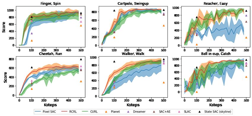
Published as a conference paper at ICLR 2021

Contrastive representation learning for Reinforcement Learning (RCRL). In our method, given an
anchor state-action pair, we choose a state-action pair with the same or similar return as the pos-
itive sample, and a state-action pair with different return as the negative sample. Then, we train
a discriminator to classify between positive and negative samples given the anchor based on their
representations as the auxiliary task. The intuition here is to learn state-action representations that
capture return-relevant features while ignoring return-irrelevant features.
From a theoretical perspective, RCRL is supported by a novel state-action abstraction, called Z π -
irrelevance. Z π -irrelevance abstraction aggregates state-action pairs with similar return distributions
under certain policy π. We show that Z π -irrelevance abstraction can reduce the size of the state-
action space (cf. Appendix A) as well as approximate the Q values arbitrarily accurately (cf. Section
4.1). We further propose a method called Z-learning that can calculate Z π -irrelevance abstraction
with sampled returns rather than the return distribution, which is hardly available in practice. Z-
learning can learn Z π -irrelevance abstraction provably efficiently. Our algorithm RCRL can be seen
as the empirical version of Z-learning by making a few approximations such as integrating with
deep RL algorithms, and collecting positive pairs within a consecutive segment in a trajectory of the
anchors.
We conduct experiments on Atari games (Bellemare et al., 2013) and DeepMind Control suite (Tassa
et al., 2018) in low data regime. The experiment results show that our auxiliary task combined with
Rainbow (Hessel et al., 2017) for discrete control tasks or SAC (Haarnoja et al., 2018) for continuous
control tasks achieves superior performance over other state-of-the-art baselines for this regime. Our
method can be further combined with existing unsupervised contrastive learning methods to achieve
even better performance. We also perform a detailed analysis on how the representation changes
during training with/without our auxiliary loss. We find that a good embedding network assigns
similar/dissimilar representations to state-action pairs with similar/dissimilar return distributions,
and our algorithm can boost such generalization and speed up training.
Our contributions are summarized as follows:
       • We introduce a novel contrastive loss based on return, to learn return-relevant representa-
         tions and speed up deep RL algorithms.
       • We theoretically build the connection between the contrastive loss and a new form of state-
         action abstraction, which can reduce the size of the state-action space as well as approxi-
         mate the Q values arbitrarily accurately.
       • Our algorithm achieves superior performance against strong baselines in Atari games and
         DeepMind Control suite in low data regime. Besides, the performance can be further en-
         hanced when combined with existing auxiliary tasks.

2     R ELATED W ORK
2.1   AUXILIARY TASK

In reinforcement learning, the auxiliary task can be used for both the model-based setting and the
model-free setting. In the model-based settings, world models can be used as auxiliary tasks and lead
to better performance, such as CRAR (François-Lavet et al., 2019), Dreamer (Hafner et al., 2019a),
and PlaNet (Hafner et al., 2019b). Due to the complex components (e.g., the latent transition or
reward module) in the world model, such methods are empirically unstable to train and relies on
different regularizations to converge. In the model-free settings, many algorithms construct various
auxiliary tasks to improve performance, such as predicting the future (Jaderberg et al., 2016; Shel-
hamer et al., 2016; Guo et al., 2020; Lee et al., 2020; Mazoure et al., 2020), learning value functions
with different rewards or under different policies (Veeriah et al., 2019; Schaul et al., 2015; Borsa
et al., 2018; Bellemare et al., 2019; Dabney et al., 2020), learning from many-goals (Veeriah et al.,
2018), or the combination of different auxiliary objectives (de Bruin et al., 2018). Moreover, aux-
iliary tasks can be designed based on the prior knowledge about the environment (Mirowski et al.,
2016; Shen et al., 2020; van der Pol et al., 2020) or the raw state representation (Srinivas et al.,
2020). Hessel et al. (2019) also apply auxiliary task to the multi-task RL setting.
Contrastive learning has seen dramatic progress recently, and been introduced to learn state repre-
sentation (Oord et al., 2018; Sermanet et al., 2018; Dwibedi et al., 2018; Aytar et al., 2018; Anand

                                                   2
Published as a conference paper at ICLR 2021
et al., 2019; Srinivas et al., 2020). Temporal structure (Sermanet et al., 2018; Aytar et al., 2018) and
local spatial structure (Anand et al., 2019) has been leveraged for state representation learning via
contrastive losses. CPC (Oord et al., 2018) and CURL (Srinivas et al., 2020) adopt a contrastive
auxiliary tasks to accelerate representation learning and speed up main RL tasks, by leveraging the
temporal structure and image augmentation respectively. To the best of our knowledge, we are the
first to leverage return to construct a contrastive auxiliary task for speeding up the main RL task.
2.2 A BSTRACTION
State abstraction (or state aggregation) aggregates states by ignoring irrelevant state information.
By reducing state space, state abstraction can enable efficient policy learning. Different types of
abstraction are proposed in literature, ranging from fine-grained to coarse-grained abstraction, each
reducing state space to a different extent. Bisimulation or model irrelevance (Dean and Givan, 1997;
Givan et al., 2003) define state abstraction under which both transition and reward function are kept
invariant. By contrast, other types of state abstraction that are coarser than bisimulation such as Qπ
irrelevance or Q∗ irrelevance (see e.g., Li et al., 2006), which keep the Q function invariant under any
policy π or the optimal policy respectively. There are also some works on state-action abstractions,
e.g., MDP homomorphism (Ravindran, 2003; Ravindran and Barto, 2004a) and approximate MDP
homomorphism (Ravindran and Barto, 2004b; Taylor et al., 2009) , which are similar to bisimulation
in keeping reward and transition invariant, but extending bisimulation from state abstraction to state-
action abstraction.
In this paper, we consider a new form of state-action abstraction Z π -irrelevance, which aggregates
state-action pairs with the same return distribution and is coarser than bisimulation or homomor-
phism which are frequently used as auxiliary tasks (e.g., Biza and Platt, 2018; Gelada et al., 2019;
Zhang et al., 2020). However, it is worth noting that Z π -irrelevance is only used to build the theo-
retical foundation of our algorithm, and show that our proposed auxiliary task is well-aligned with
the main RL task. Representation learning in deep RL is in general very different from aggregating
states in tabular case, though the latter may build nice theoretical foundation for the former. Here
we focus on how to design auxiliary tasks to accelerate representation learning using contrastive
learning techniques, and we propose a novel return-based contrastive method based on our proposed
Z π -irrelevance abstraction.
3 P RELIMINARY
We consider a Markov Decision Process (MDP) which is a tuple (S, A, P, R, µ, γ) specifying
the state space S, the action space A, the state transition probability P (st+1 |st , at ), the reward
R(rt |st , at ), the initial state distribution µ ∈ ∆S and the discount factor γ. Also, we denote
x := (s, a) ∈ X := S × A to be the state-action pair. A (stationary) policy π : S → ∆A specifies
the action selection probability on each state. Following the policy π,P∞ the discounted sum of future
rewards (or return) is denoted by the random variable Z π (s, a) = t=0 γ t R(st , at ), where s0 =
s, a0 = a, st ∼ P (·|st−1 , at−1 ), and at ∼ π(·|st ). We divide the range of return into K equal bins
{R0 = Rmin , R1 , · · · , RK = Rmax } such that Rk − Rk−1 = (Rmax − Rmin )/K, ∀k ∈ [K], where
Rmin (resp. Rmax ) is the minimum (reps. maximum) possible return, and [K] := {1, 2, · · · , K}.
We use b(R) = k ∈ [K] to denote the event that R falls into the kth bin, i.e., Rk−1 < R ≤ Rk .
Hence, b(R) can be viewed as the discretized version of the return, and the distribution of discretized
return can be represented by a K-dimensional vector Zπ (x) ∈ ∆K , where the k-th element equals
to Pr[Rk−1 < Z π (x) ≤ Rk ]. The Q function is defined as Qπ (x) = E[Z π (x)], and the state value
function is defined as V π (s) = Ea∼π(·|s) [Z π (s, a)]. The objective for RL is to find a policy π that
maximizes the expected cumulative reward J(π) = Es∼µ [V π (s)]. We denote the optimal policy as
∗
π ∗ and the corresponding optimal Q function as Q∗ := Qπ .
4 M ETHODOLOGY
In this section, we present our method, from both theoretical and empirical perspectives. First, we
propose Z π -irrelevance, a new form of state-action abstraction based on return distribution. We
show that the Q functions for any policy (and therefore the optimal policy) can be represented under
3Published as a conference paper at ICLR 2021
Algorithm 1: Z-learning
1: Given the policy π, the number of bins for the return K, a constant N ≥ Nπ,K , the encoder
class ΦN , the regressor class WN , and a distribution d ∈ ∆X with supp(d) = X
2: D = ∅
3: for i = 1, · · · , n do
4: x1 , x2 ∼ d
5: R1 ∼ Z π (x1 ), R2 ∼ Z π (x2 )
6: D = D ∪ {(x1 , x2 , y = I[b(R1 ) 6= b(R2 )])}
7: end for
8: (φ̂, ŵ) = arg minφ∈ΦN ,w∈WN L(φ, w; D), where L(φ, w; D) is defined in (1)
9: return the encoder φ̂
Z π -irrelevance abstraction. Then we consider an algorithm, Z-learning, that enables us to learn
Z π -irrelevance abstraction from the samples collected using π. Z-learning is simple and learns the
abstraction by only minimizing a contrastive loss. We show that Z-learning can learn Z π -irrelevance
abstraction provably efficiently. After that, we introduce return-based contrastive representation
learning for RL (RCRL) that incorporates standard RL algorithms with an auxiliary task adapted
from Z-learning. At last, we present our network structure for learning state-action embedding,
upon which RCRL is built.
4.1 Z π - IRRELEVANCE A BSTRACTION
A state-action abstraction aggregates the state-action pairs with similar properties, resulting in an
abstract state-action space denoted as [N ], where N is the size of abstract state-action space. In
this paper, we consider a new form of abstraction, Z π -irrelevance, defined as follows: Given a
policy π, Z π -irrelevance abstraction is denoted as φ : X → [N ] such that, for any x1 , x2 ∈ X
with φ(x1 ) = φ(x2 ), we have Zπ (x1 ) = Zπ (x2 ). Given a policy π and the parameter for return
discretization K, we use Nπ,K to denote the minimum N such that a Z π -irrelevance exists. It is
true that Nπ,K ≤ Nπ,∞ ≤ |φB (S)| |A| for any π and K, where |φB (S)| is the number of abstract
states for the coarsest bisimulation (cf. Appendix A).
Proposition 4.1. Given a policy π and any Z π -irrelevance φ : X → [N ], there exists a function
−Rmin
Q : [N ] → R such that |Q(φ(x)) − Qπ (x)| ≤ RmaxK , ∀x ∈ X .
We provide a proof in Appendix A. Note that K controls the coarseness of the abstraction. When
K → ∞, Z π -irrelevance can accurately represent the value function and therefore the optimal policy
when π → π ∗ . When using an auxiliary task to learn such abstraction, this proposition indicates that
the auxiliary task (to learn a Z π -irrelevance) is well-aligned with the main RL task (to approximate
Q∗ ). However, large K results in a fine-grained abstraction which requires us to use a large N and
more samples to learn the abstraction (cf. Theorem 4.1). In practice, this may not be a problem
since we learn a state-action representation in a low-dimensional space Rd instead of [N ] and reuse
the samples collected by the base RL algorithm. Also, we do not need to choose a K explicitly in
the practical algorithm (cf. Section 4.3).
4.2 Z-L EARNING
We propose Z-learning to learn Z π -irrelevance based on a dataset D with a contrastive loss (see
Algorithm 1). Each tuple in the dataset is collected as follows: First, two state-action pairs are drawn
i.i.d. from a distribution d ∈ ∆X with supp(d) = X (cf. Line 4 in Algorithm 1). In practice, we
can sample state-action pairs from the rollouts generated by the policy π. In this case, a stochastic
policy (e.g., using -greedy) with a standard ergodic assumption on MDP ensures supp(d) = X .
Then, we obtain returns for the two state-action pairs (i.e., the discounted sum of the rewards after
x1 and x2 ) which can be obtained by rolling out using the policy π (cf. Line 5 in Algorithm 1). The
binary label y for this state-action pair indicates whether the two returns belong to the same bin (cf.
Line 6 in Algorithm 1). The contrastive loss is defined as follows:
L(φ, w; D) := E(x1 ,x2 ,y)∼D (w(φ(x1 ), φ(x2 )) − y)2 ,
min (1)
φ∈ΦN ,w∈WN
4Published as a conference paper at ICLR 2021
where the class of encoders that map the state-action pairs to N discrete abstractions is defined as
ΦN := {X → [N ]}, and the class of tabular regressors is defined as WN := {[N ] × [N ] → [0, 1]}.
Notice that we choose N ≥ Nπ,K to ensure that a Z π -irrelevance φ : X → [N ] exists. Also, to
aggregate the state-action pairs, N should be smaller than |X | (otherwise we will obtain an identity
mapping). In this case, mapping two state-action pairs with different return distributions to the
same abstraction will increase the loss and therefore is avoided. The following theorem shows that
Z-learning can learn Z π -irrelevance provably efficiently.
Theorem 4.1. Given the encoder φ̂ returned by Algorithm 1, the following inequality holds with
probability 1 − δ and for any x0 ∈ X :
h i
Ex1 ∼d,x2 ∼d I[φ̂(x1 ) = φ̂(x2 )] Zπ (x0 )T (Zπ (x1 ) − Zπ (x2 ))
r (2)
8N 2
≤ 3 + 4N 2 ln n + 4 ln |ΦN | + 4 ln( ) ,
n δ
where |ΦN | is the cardinality of encoder function class and n is the size of the dataset.
We provide the proof in Appendix B. Although |ΦN | is upper bounded by N |X | , it is generally
much smaller for deep encoders that generalize over the state-action space. The theorem shows
that whenever φ̂ maps two state-actions x1 , x2 to the same abstraction, Zπ (x1 ) ≈ Zπ (x2 ) up to an
√
error proportional to 1/ n (ignoring the logarithm factor). The following corollary shows that φ̂
π
becomes a Z -irrelevance when n → ∞.
Corollary 4.1.1. The encoder φ̂ returned by Algorithm 1 with n → ∞ is a Z π -irrelevance, i.e., for
any x1 , x2 ∈ X , Zπ (x1 ) = Zπ (x2 ) if φ̂(x1 ) = φ̂(x2 ).
4.3 R ETURN - BASED CONTRASTIVE LEARNING FOR RL (RCRL)
We adapt Z-learning as an auxiliary task that helps the agent to learn a representation with mean-
ingful semantics. The auxiliary task based RL algorithm is called RCRL and shown in Algorithm
2. Here, we use Rainbow (for discrete control) and SAC (for continuous control) as the base RL
algorithm for RCRL. However, RCRL can also be easily incorporated with other model-free RL
algorithms. While Z-learning relies on a dataset sampled by rolling out the current policy, RCRL
constructs such a dataset using the samples collected by the base RL algorithm and therefore does
not require additional samples, e.g., directly using the replay buffer in Rainbow or SAC (see Line 7
and 8 in Algorithm 2). Compared with Z-learning, we use the state-action embedding network that is
shared with the base RL algorithm φ : X → Rd as the encoder, and use an additional discriminator
trained by the auxiliary task w : Rd × Rd → [0, 1] as the regressor.
However, when implementing Z-learning as the auxiliary task, the labels in the dataset may be
unbalanced. Although this does not cause problems in the theoretical analysis since we assume
the Bayes optimizer can be obtained for the contrastive loss, it may prevent the discriminator from
learning properly in practice (cf. Line 8 in Algorithm 1). To solve this problem, instead of drawing
samples independently from the replay buffer B (analogous to sampling from the distribution d
in Z-learning), we sample the pairs for D as follows: As a preparation, we cut the trajectories in
B into segments, where each segment contains state-action pairs with the same or similar returns.
Specifically, in Atari games, we create a new segment once the agent receives a non-zero reward. In
DMControl tasks, we first prescribe a threshold and then create a new segment once the cumulative
reward within the current segment exceeds this threshold. For each sample in D, we first draw an
anchor state-action pair from B randomly. Afterwards, we generate a positive sample by drawing
a state-action pair from the same segment of the anchor state-action pair. Then, we draw another
state-action pair randomly from B and use it as the negative sample.
We believe our auxiliary task may boost the learning, due to better return-induced representations
that facilitate generalization across different state-action pairs. Learning on one state-action pair will
affect the value of all state-action pairs that share similar representations with this pair. When the
embedding network assigns similar representations to similar state-action pairs (e.g., sharing similar
distribution over returns), the update for one state-action pair is representative for the updates for
other similar state-action pairs, which improves sample efficiency. However, such generalization
may not be achieved by the base RL algorithm since, when trained by the algorithm with only a
5Published as a conference paper at ICLR 2021
Algorithm 2: Return based Contrastive learning for RL (RCRL)
1 Initialize the embedding φθ : X → Rd and a discriminator wϑ : Rd × Rd → [0, 1]
2 Initialize the parameters ϕ for the base RL algorithm that uses the learned embedding φθ
3 Given a batch of samples D, the loss function for the base RL algorithm is LRL (φθ , ϕ; D)
4 A replay buffer B = ∅
5 foreach iteration do
6 Rollout the current policy and store the samples to the replay buffer B
7 Draw a batch of samples D from the replay buffer B
8 Update the parameters with the loss function L(φθ , wϑ ; D) + LRL (φθ , ϕ; D)
9 end
10 return The learned policy
return-based loss, similar state-action pairs may have similar Q values but very different represen-
tations. One may argue that, we can adopt several temporal difference updates to propagate the
values for state-action pairs with same sampled return, and finally all such pairs are assigned with
similar Q values. However, since we adopt a learning algorithm with bootstrapping/temporal differ-
ence learning and frozen target network in deep RL, it could take longer time to propagate the value
across different state-action pairs, compared with direct generalization over state-action pairs with
contrastive learning.
Meanwhile, since we construct auxiliary tasks based on return, which is a very different structure
from image augmentation or temporal structure, our method could be combined with existing meth-
ods to achieve further improvement.
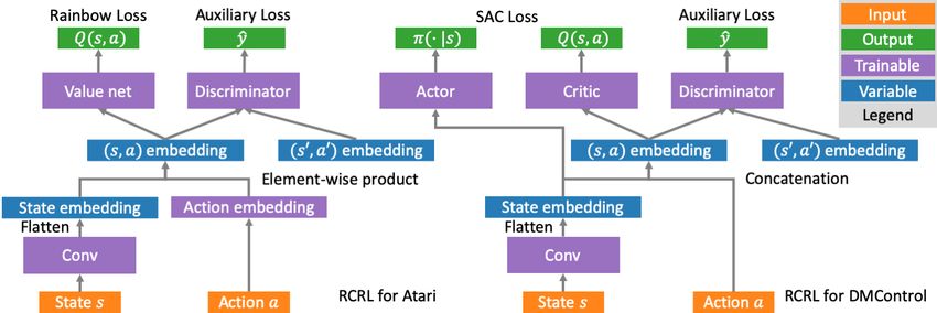
4.4 N ETWORK S TRUCTURE FOR S TATE - ACTION E MBEDDING
In our algorithm, the auxiliary task is based on the state-action embedding, instead of the state
embedding that is frequently used in the previous work (e.g., Srinivas et al., 2020). To facilitate
our algorithm, we design two new structures for Atari 2600 Games (discrete action) and DMControl
Suite (continuous action) respectively. We show the structure in Figure 1. For Atari, we learn an
action embedding for each action and use the element-wise product of the state embedding and
action embedding as the state-action embedding. For DMControl, the action embedding is a real-
valued vector and we use the concatenation of the action embedding and the state embedding.
Figure 1: The network structure of RCRL for Atari (left) and DMControl Suite (right).
5 E XPERIMENT
In this section, we conduct the following experiments: 1) We implement RCRL on Atari 2600
Games (Bellemare et al., 2013) and DMControl Suite (Tassa et al., 2020), and compare with state-
of-the-art model-free methods and strong model-based methods. In particular, we compare with
CURL (Srinivas et al., 2020), a top performing auxiliary task based RL algorithm for pixel-based
control tasks that also uses a contrastive loss. In addition, we also combine RCRL with CURL to
study whether our auxiliary task further boosts the learning when combined with other auxiliary
6Published as a conference paper at ICLR 2021
tasks. 2) To further study the reason why our algorithm works, we analyze the generalization of the
learned representation. Specifically, we compare the cosine similarity between the representations
of different state-action pairs. We provide the implementation details in Appendix C.
5.1 E VALUATION ON ATARI AND DMC ONTROL
Experiments on Atari. Our experiments on Atari are conducted in low data regime of 100k in-
teractions between the agent and the environment, which corresponds to two hours of human play.
We show the performance of different algorithms/baselines, including the scores for average human
(Human), SimPLe (Kaiser et al., 2019) which is a strong model-based baseline for this regime, orig-
inal Rainbow (Hessel et al., 2017), Data-Efficient Rainbow (ERainbow, van Hasselt et al., 2019),
ERainbow with state-action embeddings (ERainbow-sa, cf. Figure 1 Left), CURL (Srinivas et al.,
2020) that is based on ERainbow, RCRL which is based on ERainbow-sa, and the algorithm that
combines the auxiliary loss for CURL and RCRL to ERainbow-sa (RCRL+CURL). We show the
evaluation results of our algorithm and the baselines on Atari games in Table 1. First, we observe that
using state-action embedding instead of state embedding in ERainbow does not lead to significant
performance change by comparing ERainbow with ERainbow-sa. Second, built upon ERainbow-sa,
the auxiliary task in RCRL leads to better performance compared with not only the base RL algo-
rithm but also SimPLe and CURL in terms of the median human normalized score (HNS). Third, we
can see that RCRL further boosts the learning when combined with CURL and achieves the best per-
formance for 7 out of 26 games, which shows that our auxiliary task can be successfully combined
with other auxiliary tasks that embed different sources of information to learn the representation.
Human SimPLe Rainbow ERainbow ERainbow-sa CURL RCRL RCRL+CURL
ALIEN 7127.7 616.9 318.7 739.9 813.8 558.2 854.2 912.2
AMIDAR 1719.5 88.0 32.5 188.6 154.2 142.1 157.7 125.1
ASSAULT 742.0 527.2 231.0 431.2 576.2 600.6 569.6 588.4
ASTERIX 8503.3 1128.3 243.6 470.8 697.0 734.5 799.0 683.0
BANK HEIST 753.1 34.2 15.6 51.0 96.0 131.6 107.2 99.0
BATTLE ZONE 37187.5 5184.4 2360.0 10124.6 13920.0 14870.0 14280.0 17380.0
BOXING 12.1 9.1 -24.8 0.2 2.2 1.2 2.7 6.7
BREAKOUT 30.5 16.4 1.2 1.9 3.4 4.9 4.3 4.0
CHOPPER COMMAND 7387.8 1246.9 120.0 861.8 1064.0 1058.5 1262.0 1008.0
CRAZY CLIMBER 35829.4 62583.6 2254.5 16185.3 21840.0 12146.5 15120.0 15032.0
DEMON ATTACK 1971.0 208.1 163.6 508.0 768.0 817.6 790.4 618.3
FREEWAY 29.6 20.3 0.0 27.9 26.5 26.7 26.6 25.4
FROSTBITE 4334.7 254.7 60.2 866.8 1472.0 1181.3 1337.6 1516.6
GOPHER 2412.5 771.0 431.2 349.5 384.8 669.3 429.6 458.8
HERO 30826.4 2656.6 487.0 6857.0 4787.9 6279.3 6454.1 7647.4
JAMESBOND 302.8 125.3 47.4 301.6 308.0 471.0 314.0 503.0
KANGAROO 3035.0 323.1 0.0 779.3 732.0 872.5 842.0 932.0
KRULL 2665.5 4539.9 1468.0 2851.5 2740.0 4229.6 2997.5 3905.8
KUNG FU MASTER 22736.3 17257.2 0.0 14346.1 11914.0 14307.8 9762.0 11856.0
MS PACMAN 6951.6 1480.0 67.0 1204.1 1384.5 1465.5 1555.2 1336.8
PONG 14.6 12.8 -20.6 -19.3 -18.3 -16.5 -16.9 -18.72
PRIVATE EYE 69571.3 58.3 0.0 97.8 80.0 218.4 102.6 282.3
QBERT 13455.0 1288.8 123.5 1152.9 893.5 1042.4 1121.0 942.0
ROAD RUNNER 7845.0 5640.6 1588.5 9600.0 5392.0 5661.0 6138.0 5392.0
SEAQUEST 42054.7 683.3 131.7 354.1 402.0 384.5 375.6 489.6
UP N DOWN 11693.2 3350.3 504.6 2877.4 3235.2 2955.2 4210.2 3127.8
Median HNS 100.0% 14.4% 0.0% 16.1% 16.7% 17.5% 18.5% 19.6%
Table 1: Scores of different algorithms/baselines on 26 games for Atari-100k benchmark. We show
the mean score averaged over five random seeds.
Experiments on DMControl. For DMControl, we compare our algorithm with the following base-
lines: Pixel SAC (Haarnoja et al., 2018) which is the base RL algorithm that receives images as
the input; SLAC (Lee et al., 2019) that learns a latent variable model and then updates the actor
and critic based on it; SAC+AE (Yarats et al., 2019) that uses a regularized autoencoder for recon-
struction in the auxiliary task; PlaNet (Hafner et al., 2019b) and Dreamer (Hafner et al., 2019a) that
learn a latent space world model and explicitly plan with the learned model. We also compare with
a skyline, State SAC, the receives the low-dimensional state representation instead of the image as
the input. Different from Atari games, tasks in DMControl yield dense reward. Consequently, we
split the trajectories into segments using a threshold such that the difference of returns within each
segment does not exceed this threshold. Similarly, we test the algorithms in low data regime of 500k
interactions. We show the evaluation results in Figure 2. We can see that our auxiliary task not only
brings performance improvement over the base RL algorithm but also outperforms CURL and other
state-of-the-art baseline algorithms in different tasks. Moreover, we observe that our algorithm is
7Published as a conference paper at ICLR 2021
Figure 2: Scores achieved by RCRL and other baseline algorithms during the training for differ-
ent tasks in DMControl suite. The line and the shaded area indicate the average and the standard
deviation over 5 random seeds respectively.
more robust across runs with different seeds compared with Pixel SAC and CURL (e.g., for the task
Ball in cup, Catch).
5.2 A NALYSIS ON THE LEARNED REPRESENTATION
We analyze on the learned representation of our model to demonstrate that our auxiliary task at-
tains a representation with better generalization, which may explain why our algorithm succeeds.
We use cosine similarity to measure the generalization from one state-action pair to another in the
deep learning model. Given two state-action pairs x1 , x2 ∈ X , cosine similarity is defined as
φθ (x1 )T φθ (x2 )
||φθ (x1 )|| ||φθ (x2 )|| , where φθ (·) is the learnt embedding network.
We show the cosine similarity of the representations between positive pairs (that are sampled within
the same segment and therefore likely to share similar return distributions) and negative pairs (i.e.,
randomly sampled state-action pairs) during the training on the game Alien in Figure 4. First, we
observe that when a good policy is learned, the representations of positive pairs are similar while
those of negative pairs are dissimilar. This indicates that a good representation (or the representation
that supports a good policy) aggregates the state-action pairs with similar return distributions. Then,
we find that our auxiliary loss can accelerate such generalization for the representation, which makes
RCRL learn faster.
Figure 3: Analysis of the learned representation on Alien. (a) The cosine similarity between the rep-
resentations of the positive/negative state-action pair and the anchor during the training of Rainbow
and RCRL. (b) The scores of the two algorithms during the training.
8Published as a conference paper at ICLR 2021
6 C ONCLUSION
In this paper, we propose return-based contrastive representation learning for RL (RCRL), which
introduces a return-based auxiliary task to facilitate policy training with standard RL algorithms.
Our auxiliary task is theoretically justified to learn representations that capture the structure of Z π -
irrelevance, which can reduce the size of the state-action space as well as approximate the Q values
arbitrarily accurately. Experiments on Atari games and the DMControl suite in low data regime
demonstrate that our algorithm achieves superior performance not only when using our auxiliary
task alone but also when combined with other auxiliary tasks, .
As for future work, we are interested in how to combine different auxiliary tasks in a more so-
phisticated way, perhaps with a meta-controller. Another potential direction would be providing a
theoretical analysis for auxiliary tasks and justifying why existing auxiliary tasks can speed up deep
RL algorithms.
7 ACKNOWLEDGMENT
Guoqing Liu and Nenghai Yu are supported in part by the Natural Science Foundation of China under
Grant U20B2047, Exploration Fund Project of University of Science and Technology of China under
Grant YD3480002001. Chuheng Zhang and Jian Li are supported in part by the National Natural
Science Foundation of China Grant 61822203, 61772297, 61632016 and the Zhongguancun Haihua
Institute for Frontier Information Technology, Turing AI Institute of Nanjing and Xi’an Institute for
Interdisciplinary Information Core Technology.
R EFERENCES
Volodymyr Mnih, Koray Kavukcuoglu, David Silver, Andrei A Rusu, Joel Veness, Marc G Belle-
mare, Alex Graves, Martin Riedmiller, Andreas K Fidjeland, Georg Ostrovski, et al. Human-level
control through deep reinforcement learning. Nature, 518(7540):529, 2015.
Aravind Srinivas, Michael Laskin, and Pieter Abbeel. Curl: Contrastive unsupervised representa-
tions for reinforcement learning. arXiv preprint arXiv:2004.04136, 2020.
Steven C Suddarth and YL Kergosien. Rule-injection hints as a means of improving network per-
formance and learning time. In European Association for Signal Processing Workshop, pages
120–129. Springer, 1990.
Richard S Sutton, Joseph Modayil, Michael Delp, Thomas Degris, Patrick M Pilarski, Adam White,
and Doina Precup. Horde: A scalable real-time architecture for learning knowledge from unsu-
pervised sensorimotor interaction. In The 10th International Conference on Autonomous Agents
and Multiagent Systems-Volume 2, pages 761–768, 2011.
Carles Gelada, Saurabh Kumar, Jacob Buckman, Ofir Nachum, and Marc G Bellemare. Deep-
mdp: Learning continuous latent space models for representation learning. arXiv preprint
arXiv:1906.02736, 2019.
Marc Bellemare, Will Dabney, Robert Dadashi, Adrien Ali Taiga, Pablo Samuel Castro, Nicolas
Le Roux, Dale Schuurmans, Tor Lattimore, and Clare Lyle. A geometric perspective on opti-
mal representations for reinforcement learning. In Advances in Neural Information Processing
Systems, pages 4358–4369, 2019.
Vincent François-Lavet, Yoshua Bengio, Doina Precup, and Joelle Pineau. Combined reinforce-
ment learning via abstract representations. In Proceedings of the AAAI Conference on Artificial
Intelligence, volume 33, pages 3582–3589, 2019.
Wei Shen, Xiaonan He, Chuheng Zhang, Qiang Ni, Wanchu Dou, and Yan Wang. Auxiliary-task
based deep reinforcement learning for participant selection problem in mobile crowdsourcing.
arXiv preprint arXiv:2008.11087, 2020.
9Published as a conference paper at ICLR 2021
Amy Zhang, Rowan McAllister, Roberto Calandra, Yarin Gal, and Sergey Levine. Learning
invariant representations for reinforcement learning without reconstruction. arXiv preprint
arXiv:2006.10742, 2020.
Will Dabney, André Barreto, Mark Rowland, Robert Dadashi, John Quan, Marc G Bellemare, and
David Silver. The value-improvement path: Towards better representations for reinforcement
learning. arXiv preprint arXiv:2006.02243, 2020.
Max Jaderberg, Volodymyr Mnih, Wojciech Marian Czarnecki, Tom Schaul, Joel Z Leibo, David
Silver, and Koray Kavukcuoglu. Reinforcement learning with unsupervised auxiliary tasks. arXiv
preprint arXiv:1611.05397, 2016.
Danijar Hafner, Timothy Lillicrap, Jimmy Ba, and Mohammad Norouzi. Dream to control: Learning
behaviors by latent imagination. arXiv preprint arXiv:1912.01603, 2019a.
Danijar Hafner, Timothy Lillicrap, Ian Fischer, Ruben Villegas, David Ha, Honglak Lee, and James
Davidson. Learning latent dynamics for planning from pixels. In International Conference on
Machine Learning, pages 2555–2565, 2019b.
Aaron van den Oord, Yazhe Li, and Oriol Vinyals. Representation learning with contrastive predic-
tive coding. arXiv preprint arXiv:1807.03748, 2018.
Marc G Bellemare, Yavar Naddaf, Joel Veness, and Michael Bowling. The arcade learning environ-
ment: An evaluation platform for general agents. Journal of Artificial Intelligence Research, 47:
253–279, 2013.
Yuval Tassa, Yotam Doron, Alistair Muldal, Tom Erez, Yazhe Li, Diego de Las Casas, David Bud-
den, Abbas Abdolmaleki, Josh Merel, Andrew Lefrancq, et al. Deepmind control suite. arXiv
preprint arXiv:1801.00690, 2018.
Matteo Hessel, Joseph Modayil, Hado Van Hasselt, Tom Schaul, Georg Ostrovski, Will Dabney, Dan
Horgan, Bilal Piot, Mohammad Azar, and David Silver. Rainbow: Combining improvements in
deep reinforcement learning. arXiv preprint arXiv:1710.02298, 2017.
Tuomas Haarnoja, Aurick Zhou, Pieter Abbeel, and Sergey Levine. Soft actor-critic: Off-policy
maximum entropy deep reinforcement learning with a stochastic actor. In Proceedings of the 35th
International Conference on Machine Learning, volume 80, pages 1861–1870. JMLR, 2018.
Evan Shelhamer, Parsa Mahmoudieh, Max Argus, and Trevor Darrell. Loss is its own reward: Self-
supervision for reinforcement learning. arXiv preprint arXiv:1612.07307, 2016.
Daniel Guo, Bernardo Avila Pires, Bilal Piot, Jean-bastien Grill, Florent Altché, Rémi Munos, and
Mohammad Gheshlaghi Azar. Bootstrap latent-predictive representations for multitask reinforce-
ment learning. arXiv preprint arXiv:2004.14646, 2020.
Kuang-Huei Lee, Ian Fischer, Anthony Liu, Yijie Guo, Honglak Lee, John Canny, and Sergio
Guadarrama. Predictive information accelerates learning in rl. arXiv preprint arXiv:2007.12401,
2020.
Bogdan Mazoure, Remi Tachet des Combes, Thang Doan, Philip Bachman, and R Devon Hjelm.
Deep reinforcement and infomax learning. arXiv preprint arXiv:2006.07217, 2020.
Vivek Veeriah, Matteo Hessel, Zhongwen Xu, Janarthanan Rajendran, Richard L Lewis, Junhyuk
Oh, Hado P van Hasselt, David Silver, and Satinder Singh. Discovery of useful questions as
auxiliary tasks. In Advances in Neural Information Processing Systems, pages 9310–9321, 2019.
Tom Schaul, Daniel Horgan, Karol Gregor, and David Silver. Universal value function approxima-
tors. In International conference on machine learning, pages 1312–1320, 2015.
Diana Borsa, André Barreto, John Quan, Daniel Mankowitz, Rémi Munos, Hado van Hasselt,
David Silver, and Tom Schaul. Universal successor features approximators. arXiv preprint
arXiv:1812.07626, 2018.
10Published as a conference paper at ICLR 2021
Vivek Veeriah, Junhyuk Oh, and Satinder Singh. Many-goals reinforcement learning. arXiv preprint
arXiv:1806.09605, 2018.
Tim de Bruin, Jens Kober, Karl Tuyls, and Robert Babuška. Integrating state representation learning
into deep reinforcement learning. IEEE Robotics and Automation Letters, 3(3):1394–1401, 2018.
Piotr Mirowski, Razvan Pascanu, Fabio Viola, Hubert Soyer, Andrew J Ballard, Andrea Banino,
Misha Denil, Ross Goroshin, Laurent Sifre, Koray Kavukcuoglu, et al. Learning to navigate in
complex environments. arXiv preprint arXiv:1611.03673, 2016.
Elise van der Pol, Daniel E Worrall, Herke van Hoof, Frans A Oliehoek, and Max Welling.
Mdp homomorphic networks: Group symmetries in reinforcement learning. arXiv preprint
arXiv:2006.16908, 2020.
Matteo Hessel, Hubert Soyer, Lasse Espeholt, Wojciech Czarnecki, Simon Schmitt, and Hado van
Hasselt. Multi-task deep reinforcement learning with popart. In Proceedings of the AAAI Confer-
ence on Artificial Intelligence, volume 33, pages 3796–3803, 2019.
Pierre Sermanet, Corey Lynch, Yevgen Chebotar, Jasmine Hsu, Eric Jang, Stefan Schaal, Sergey
Levine, and Google Brain. Time-contrastive networks: Self-supervised learning from video. In
2018 IEEE International Conference on Robotics and Automation (ICRA), pages 1134–1141.
IEEE, 2018.
Debidatta Dwibedi, Jonathan Tompson, Corey Lynch, and Pierre Sermanet. Learning actionable rep-
resentations from visual observations. In 2018 IEEE/RSJ International Conference on Intelligent
Robots and Systems (IROS), pages 1577–1584. IEEE, 2018.
Yusuf Aytar, Tobias Pfaff, David Budden, Thomas Paine, Ziyu Wang, and Nando de Freitas. Playing
hard exploration games by watching youtube. In Advances in Neural Information Processing
Systems, pages 2930–2941, 2018.
Ankesh Anand, Evan Racah, Sherjil Ozair, Yoshua Bengio, Marc-Alexandre Côté, and R Devon
Hjelm. Unsupervised state representation learning in atari. In Advances in Neural Information
Processing Systems, pages 8769–8782, 2019.
Thomas Dean and Robert Givan. Model minimization in markov decision processes. In AAAI/IAAI,
pages 106–111, 1997.
Robert Givan, Thomas Dean, and Matthew Greig. Equivalence notions and model minimization in
markov decision processes. Artificial Intelligence, 147(1-2):163–223, 2003.
Lihong Li, Thomas J Walsh, and Michael L Littman. Towards a unified theory of state abstraction
for mdps. In ISAIM, 2006.
Balaraman Ravindran. Smdp homomorphisms: An algebraic approach to abstraction in semi markov
decision processes. 2003.
Balaraman Ravindran and Andrew G Barto. An algebraic approach to abstraction in reinforcement
learning. PhD thesis, University of Massachusetts at Amherst, 2004a.
Balaraman Ravindran and Andrew G Barto. Approximate homomorphisms: A framework for non-
exact minimization in markov decision processes. 2004b.
Jonathan Taylor, Doina Precup, and Prakash Panagaden. Bounding performance loss in approximate
mdp homomorphisms. In Advances in Neural Information Processing Systems, pages 1649–1656,
2009.
Ondrej Biza and Robert Platt. Online abstraction with mdp homomorphisms for deep learning. arXiv
preprint arXiv:1811.12929, 2018.
Yuval Tassa, Saran Tunyasuvunakool, Alistair Muldal, Yotam Doron, Siqi Liu, Steven Bohez, Josh
Merel, Tom Erez, Timothy Lillicrap, and Nicolas Heess. dmcontrol: Software and tasks for
continuous control, 2020.
11Published as a conference paper at ICLR 2021
Lukasz Kaiser, Mohammad Babaeizadeh, Piotr Milos, Blazej Osinski, Roy H Campbell, Konrad
Czechowski, Dumitru Erhan, Chelsea Finn, Piotr Kozakowski, Sergey Levine, et al. Model-based
reinforcement learning for atari. arXiv preprint arXiv:1903.00374, 2019.
Hado P van Hasselt, Matteo Hessel, and John Aslanides. When to use parametric models in rein-
forcement learning? In Advances in Neural Information Processing Systems, pages 14322–14333,
2019.
Alex X Lee, Anusha Nagabandi, Pieter Abbeel, and Sergey Levine. Stochastic latent actor-critic:
Deep reinforcement learning with a latent variable model. arXiv preprint arXiv:1907.00953,
2019.
Denis Yarats, Amy Zhang, Ilya Kostrikov, Brandon Amos, Joelle Pineau, and Rob Fergus. Im-
proving sample efficiency in model-free reinforcement learning from images. arXiv preprint
arXiv:1910.01741, 2019.
Pablo Samuel Castro. Scalable methods for computing state similarity in deterministic markov
decision processes. In Proceedings of the AAAI Conference on Artificial Intelligence, volume 34,
pages 10069–10076, 2020.
Dipendra Misra, Mikael Henaff, Akshay Krishnamurthy, and John Langford. Kinematic state
abstraction and provably efficient rich-observation reinforcement learning. arXiv preprint
arXiv:1911.05815, 2019.
Marc G Bellemare, Will Dabney, and Rémi Munos. A distributional perspective on reinforcement
learning. arXiv preprint arXiv:1707.06887, 2017.
12Published as a conference paper at ICLR 2021
A Z π - IRRELEVANCE
A.1 C OMPARISON WITH BISIMULATION .
We consider a bisimulation φ and denote the set of abstract states as Z := φ(S). The bisimulation
φB is defined as follows:
Definition A.1 (Bisimulation (Givan et al., 2003)). φB is bisimulation if ∀s1 , s2 ∈ S where
φB (s1 ) = φB (s2 ), ∀a ∈ A, z 0 ∈ Z,
X X
R(s1 , a) = R(s2 , a), P (s0 |s1 , a) = P (s0 |s2 , a).
s0 ∈φ−1 0
B (z ) s0 ∈φ−1 0
B (z )
Notice that the coarseness of Z π -irrelevance is dependent on K, the number of bins for the return.
D
When K → ∞, two state-action pairs x and x0 are aggregated only when Z π (x) = Z π (x0 ), which is
a strict condition resulting in a fine-grained abstraction. Here, we provide the following proposition
to illustrate that Z π -irrelevance abstraction is coarser than bisimulation even when K → ∞.
Proposition A.1. Given φB to be the coarsest bisimulation, φB induces a Z π -irrelevance abstrac-
tion for any policy π defined over Z. Specifically, if ∀s1 , s2 ∈ S where φB (s1 ) = φB (s2 ), then
D
Z π (s1 , a) = Z π (s2 , a), ∀a ∈ A for any policy π defined over Z.
Consider a state-action abstraction φ̃B that is augmented from the coarsest bisimulation φB :
φ̃B (s1 , a1 ) = φ̃B (s2 , a2 ) if and only if φB (s1 ) = φ(s2 ) and a1 = a2 . The proposition indi-
cates that |φB (S)| |A| = |φ̃B (X )| ≥ Nπ,∞ ≥ Nπ,K for any K and for any π defined over Z,
i.e., bisimulation is no coarser than Z π -irrelevance. Note that there exists an optimal policy that is
defined over Z (Li et al., 2006). In practice, Z π -irrelevance should be far more coarser than bisimu-
lation when we only consider one specific policy π. Therefore learning a Z π -irrelevance should be
easier than learning a bisimulation.
Proof. First, for a fixed policy π : Z → ∆A , we prove that if two state distributions projected to
Z are identical, the corresponding reward distributions or the next state distributions projected to Z
will be identical. Then, we use such invariance property to prove the proposition.
The proof for the invariance property goes as follows: Consider two identical state distributions over
Z on the t-th step, P1 , P2 ∈ ∆Z such that P1 = P2 . Notice that we only require that the two state
distributions are identical when projected to Z, so therefore they may be different on S. Specifically,
if we denote the state distribution over S as P (s) = P (z)q(s|z) where φB (s) = z, the distribution
q for the two state distributions may be different. However, we will show that this is sufficient to
ensure that the corresponding state distributions on Z are identical on the next step (and therefore
the subsequent steps).
We denote R1 and R2 as the reward on the t-th step, which are random variables. The reward
distribution on the t-th step is specified as follows:
X
P (R1 = r|P1 ) = P (r|s, a)q1 (s|z)π(a|z)P1 (z)
z∈Z,a∈A,s∈S
X
= P (r|z, a)π(a|z)P1 (z)
z∈Z,a∈A (3)
X
= P (r|z, a)π(a|z)P2 (z)
z∈Z,a∈A
=P (R2 = r|P2 ),
D
for any r ∈ R, where we use the property of bisimulation, R|s, a = R|s0 , a, ∀φB (s) = φB (s0 ), in
D
the second equation. This indicates that R1 |P1 = R2 |P2 .
13Published as a conference paper at ICLR 2021
Similarly, we denote P10 and P20 as the state distribution over Z on the (t + 1)-th step. We have
X X X
0 0 0
P1 (z )|P1 = P (s |s, a) q1 (s|z)π(a|z)P1 (z)
z∈Z,a∈A s∈S s0 ∈φ−1 0
B (z )
X
= P (z 0 |z, a)π(a|z)P1 (z)
(4)
z∈Z,a∈A
X
= P (z 0 |z, a)π(a|z)P2 (z)
z∈Z,a∈A
=P20 (z 0 )|P1 ,
for any z 0 ∈ Z, where we also use the property of bisimulation in the second equation, i.e., the
quantity in the bracket equals for different s such that q(s|z) > 0 with a fixed z. This indicates that
P10 |P1 = P20 |P2 .
At last, consider two state s1 , s2 ∈ S with φB (s1 ) = φB (s2 ) = z on the first step, and we take
a ∈ A for both states on this step and later take the actions following π. We denote the subsequent
(1) (2) (2) (3) (1) (2) (2) (3)
reward and state distribution over Z as R1 , P1 , R1 , P1 , · · · and R2 , P2 , R2 , P2 , · · ·
(1)
respectively, where the superscripts indicate time steps. Therefore, we can deduce that P1 =
(1) (1) D (1) (2) (2) (2) D (2) D
P2 , R1 = R2 , P1 = P2 , R1 = R2 , · · · and therefore Z π (s1 , a) = Z π (s2 , a), ∀a ∈ A.
A.2 C OMPARISON WITH π- BISIMULATION
Similar to Z π -irrelevance, a recently proposed state abstraction π-bisimulation (Castro, 2020) is
also tied to a behavioral policy π. It is beneficial to compare the coarseness of Z π -irrelevance and
π-bisimulation. For completeness, we restate the definition of π-bisimulation.
Definition A.2 (π-bisimulation (Castro, 2020)). Given a policy π, φB,π is a π-bisimulation if
∀s1 , s2 ∈ S where φB,π (s1 ) = φB,π (s2 ),
X X
π(a|s1 )R(s1 , a) = π(a|s2 )R(s2 , a)
a a
X X X X
0
π(a|s1 ) P (s |s1 , a) = π(a|s2 ) P (s0 |s2 , a), ∀z 0 ∈ Z,
a s0 ∈φ−1 0 a s0 ∈φ−1 0
B,π (z ) B,π (z )
where Z := φB,π (S) is the set of abstract states.
However, π-bisimulation does not consider the state-action pair that is not visited under the policy
π (e.g., a state-action pair (s, a) when π(a|s) = 0), whereas Z π -irrelevance is defined on all the
state-action pairs. Therefore, it is hard to build connection between them unless we also define
Z π -irrelevance on the state space (instead of the state-action space) in a similar way.
Definition A.3 (Z π -irrelevance on the state space). Given s ∈ S, we denote Zπ (s) :=
π
(s, a). Given a policy π, φ is a Z π -irrelevance if ∀s1 , s2 ∈ S where φ(s1 ) = φ(s2 ),
P
a π(a|s)Z
π π
Z (s1 ) = Z (s2 ).
Based on the above definitions, the following proposition indicates that such Z π -irrelevance is
coarser than π-bisimulation.
Proposition A.2. Given a policy π and φB,π to be the coarsest π-bisimulation, if ∀s1 , s2 ∈ S where
φB,π (s1 ) = φB,π (s2 ), then Zπ (s1 ) = Zπ (s2 ).
14Published as a conference paper at ICLR 2021
Proof. Starting from s1 and s2 and following the policy π, the reward distribution and the state
distribution over Z on each step are identical, which can be proved by induction. Then, we can
D
conclude that Z π (s1 ) = Z π (s2 ) and thus Zπ (s1 ) = Zπ (s2 ).
A.3 B OUND ON THE REPRESENTATION ERROR
For completeness, we restate Proposition 4.1.
Proposition A.3. Given a policy π and any Z π -irrelevance φ : X → [N ], there exists a function
−Rmin
Q : [N ] → R such that |Q(φ(x)) − Qπ (x)| ≤ RmaxK , ∀x ∈ X .
Proof. Given a policy π and a Z π irrelevance φ, we can construct a Q such that Q(φ(x)) =
Qπ (x), ∀x ∈ X in the following way: For all x ∈ X , one by one, we assign Q(z) ← Qπ (x),
where z = φ(x). In this way, for any x ∈ X with z = φ(x), Q(z) = Qπ (x0 ) for some x0 ∈ X such
−Rmin
that Zπ (x0 ) = Zπ (x). This implies that |Q(z) − Qπ (x)| = |Qπ (x0 ) − Qπ (x)| ≤ RmaxK . This
also applies to the optimal policy π ∗ .
B P ROOF
Notice that Corollary 4.1.1 is the asymptotic case (n → ∞) for Theorem 4.1. We first provide a
sketch proof for Corollary 4.1.1 which ignores sampling issues and thus more illustrative. Later, we
provide the proof for Theorem 4.1 which mainly follows the techniques used in Misra et al. (2019).
B.1 P ROOF OF C OROLLARY 4.1.1
Recall that Z-learning aims to solve the following optimization problem:
L(φ, w; D) := E(x1 ,x2 ,y)∼D (w(φ(x1 ), φ(x2 )) − y)2 ,
min (5)
φ∈ΦN ,w∈WN
which can also be regarded as finding a compound predictor f (·, ·) := w(φ(·), φ(·)) over the func-
tion class FN := {(x1 , x2 ) → w(φ(x1 ), φ(x2 )) : w ∈ WN , φ ∈ ΦN }.
For the first step, it is helpful to find out the Bayes optimal predictor f ∗ when size of the dataset is
infinite. We notice the fact that the Bayes optimal predictor for a square loss is the conditional mean,
i.e., given a distribution D, the Bayes optimal predictor f ∗ = arg minf E(x,y)∼D [(f (x) − y)2 ]
satisfies f ∗ (x0 ) = E(x,y)∼D [y | x = x0 ]. Using this property, we can obtain the Bayes optimal
predictor over all the functions {X × X → [0, 1]} for our contrastive loss:
f ∗ (x1 , x2 ) = E(x01 ,x02 ,y)∼D [y | x01 = x1 , x02 = x2 ]
= ER1 ∼Z π (x1 ),R2 ∼Z π (x2 ) I[b(R1 ) 6= b(R2 )] (6)
π T π
= 1 − Z (x1 ) Z (x2 ),
where we use D to denote the distribution from which each tuple in the dataset D is drawn.
To establish the theorem, we require that such an optimal predictor f ∗ to be in the function class
FN . Following a similar argument to Proposition 10 in Misra et al. (2019), it is not hard to show
that using N > Nπ,K is sufficient for this realizability condition to hold.
Corollary 4.1.1. The encoder φ̂ returned by Algorithm 1 with n → ∞ is a Z π -irrelevance, i.e., for
any x1 , x2 ∈ X , Zπ (x1 ) = Zπ (x2 ) if φ̂(x1 ) = φ̂(x2 ).
Proof of Corollary 4.1.1. Considering the asymptotic case (i.e., n → ∞), we have fˆ = f ∗ where
fˆ(·, ·) := ŵ(φ̂(·), φ̂(·)) and ŵ and φ̂ is returned by Algorithm 1. If φ̂(x1 ) = φ̂(x2 ), we have for any
x ∈ X,
1 − Zπ (x1 )T Z π (x) = f ∗ (x1 , x) = fˆ(x1 , x) = fˆ(x2 , x) = f ∗ (x2 , x) = 1 − Zπ (x2 )T Zπ (x).
We obtain Zπ (x1 ) = Zπ (x2 ) by letting x = x1 or x = x2 .
15Published as a conference paper at ICLR 2021
B.2 P ROOF OF T HEOREM 4.1
Theorem 4.1. Given the encoder φ̂ returned by Algorithm 1, the following inequality holds with
probability 1 − δ and for any x0 ∈ X :
h i
Ex1 ∼d,x2 ∼d I[φ̂(x1 ) = φ̂(x2 )] Zπ (x0 )T (Zπ (x1 ) − Zπ (x2 ))
r (7)
8N 2
≤ 3 + 4N 2 ln n + 4 ln |ΦN | + 4 ln( ) ,
n δ
where |ΦN | is the cardinality of encoder function class and n is the size of the dataset.
The theorem shows that 1) whenever φ̂ maps two state-actions
√ x1 , x2 to the same abstraction,
Zπ (x1 ) ≈ Zπ (x2 ) up to an error proportional to 1/ n (ignoring the logarithm factor), and 2)
when the difference of the return distributions (e.g., Zπ (x1 ) − Zπ (x2 )) is large, the chance that two
state-action pairs (e.g., x1 and x2 ) are assigned with the same encoding is small. However, since
state-action pairs are sampled i.i.d. from the distribution d, the bound holds in an average sense
instead of the worse-case sense.
The overview of the proof is as follows: Note that the theorem builds connection between the opti-
mization problem defined in equation 5 and the learned encoder φ̂. To prove the theorem, we first
find out the minimizer f ∗ of the optimization problem when the number of samples is infinite (which
was calculated in equation 6 in the previous subsection). Then, we bound the difference between the
learned predictor fˆ and f ∗ in Lemma B.2 (which utilizes Lemma B.1) when the number of samples
is finite. At last, utilizing the compound structure of fˆ, we can relate it to the encoder φ̂. Specifically,
given x1 , x2 ∈ X with φ̂(x1 ) = φ̂(x2 ), we have fˆ(x1 , x0 ) = fˆ(x2 , x0 ), ∀x0 ∈ X .
Definition B.1 (Pointwise covering number). Given a function class G : X → R, the pointwise
covering number at scale , N (G, ), is the size of the set V : X → R such that ∀g ∈ G, ∃v ∈ V :
supx∈X |g(x) − v(x)| < .
Lemma B.1. The logarithm of the pointwise covering number of the function class FN satisfies
ln N (FN , ) ≤ N 2 ln( 1 ) + ln |ΦN |.
Proof. Recall that FN := {(x1 , x2 ) → w(φ(x1 ), φ(x2 )) : w ∈ WN , φ ∈ ΦN }, where WN :=
{[N ] × [N ] → [0, 1]} and ΦN := {X → [N ]}. Given > 0, we discretize [0, 1] to Y :=
{, · · · , d 1 e}. Then, we define WN := {[N ]×[N ] → Y } and it is easy to see that WN is a covering
2
of WN with |WN | ≤ ( 1 )N . Next, we observe that FN := {(x1 , x2 ) → w(φ(x1 ), φ(x2 )) : w ∈
WN , φ ∈ ΦN } is a covering of FN and |FN | = |ΦN | |WN |. We complete the proof by combining
the above results.
Proposition B.1 (Proposition 12 in Misra et al. (2019)). Consider a function class G : X → R
and n samples {(xi , yi )}ni=1 drawn from D, where xi ∈ X and yi ∈ [0, 1]. The Bayes op-
timal function is g ∗ = arg ming∈G E(x,y)∼D (g(x) − y)2 and the empirical risk minimizer is
1
Pn 2
ĝ = arg ming∈G n i=1 (g(xi ) − yi ) . With probability at least 1 − δ for a fixed δ ∈ (0, 1),
8 ln(2N (G, )/δ)
E(x,y)∼D (ĝ(x) − g ∗ (x))2 ≤ inf 6 +
,
>0 n
Lemma B.2. Given the empirical risk minimizer fˆ in Algorithm 1, we have
h
ˆ ∗ 2
i 6 8 2 2
E(x1 ,x2 )∼D (f (x1 , x2 ) − f (x1 , x2 )) ≤ ∆reg = + N ln n + ln |ΦN | + ln( ) , (8)
n n δ
with probability at least 1 − δ.
Proof. This directly follows from the combination of Lemma B.1 and Proposition B.1 by letting
= n1 .
16You can also read