Cumulonimbus cloud detection with weather radar at Helsinki-Vantaa airport - Helda
←
→
Page content transcription
If your browser does not render page correctly, please read the page content below
Master’s thesis
      Master’s Programme in Atmospheric Sciences
                       Meteorology

  Cumulonimbus cloud detection with
weather radar at Helsinki-Vantaa airport

                     Laura Tuomola

                     March 22, 2021

          Supervisors: Ph.D. Jussi Ylhäisi
                         Prof. Heikki Järvinen

          Examiners:     Prof. Heikki Järvinen
                         Dos. Marja Bister

                 University of Helsinki
                  Faculty of science
             PL 64 (Gustaf Hällströmin katu 2a)
                  00014 Helsingin yliopisto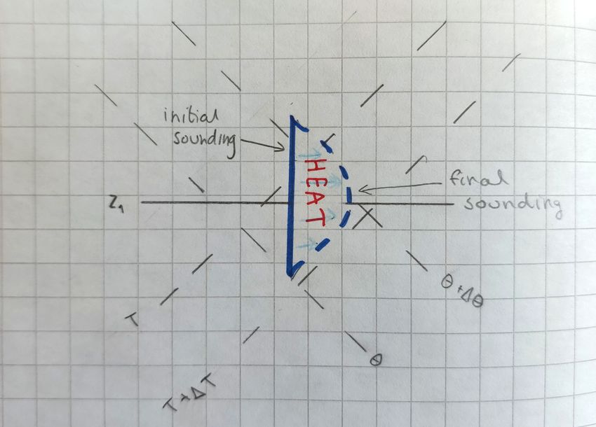
HELSINGIN YLIOPISTO — HELSINGFORS UNIVERSITET — UNIVERSITY OF HELSINKI
Tiedekunta — Fakultet — Faculty                                 Koulutusohjelma — Utbildningsprogram — Degree programme
                                                                Master’s Programme in Atmospheric Sciences
Faculty of science                                              Meteorology
Tekijä — Författare — Author

Laura Tuomola
Työn nimi — Arbetets titel — Title

Cumulonimbus cloud detection with weather radar at Helsinki-Vantaa airport
Työn laji — Arbetets art — Level             Aika — Datum — Month and year          Sivumäärä — Sidantal — Number of pages

Master’s thesis                              March 22, 2021                         42
Tiivistelmä — Referat — Abstract

Cumulonimbus (Cb) clouds form a serious threat to aviation as they can produce severe weather
hazards. Therefore, it is important to detect Cb clouds as well as possible. Finnish Meteorological
Institute (FMI) provides aeronautical meteorological services in Finland, including METeorological
Aerodrome Report (METAR). METAR describes weather at the aerodrome and its vicinity.
Significant weather is reported in METARs, and therefore Cb clouds must be included in it. At
Helsinki-Vantaa METARs are done manually by human observer. Sometimes Cb detection can
be more difficult, for example, when it is dark, and it is also expensive to have human observers
working around the clock all year round. Therefore, automation of Cb detection is a topical matter.

FMI is applying an algorithm that uses weather radar observations to detect Cb clouds.
This thesis studies how well the algorithm can detect Cb clouds compared to manual observations.
The dataset used in this thesis contains summer months (June, July and August) from 2016 to
2020. Various verification scores can be calculated to analyse the results. In addition, daytime
and night-time differences are calculated as well as different years and months are compared
together. The results show that the algorithm is not adequate to replace human observers at
Helsinki-Vantaa. However, the algorithm could be improved, for instance, by adding satellite
observations to improve detection accuracy.

Avainsanat — Nyckelord — Keywords

Meteorology, cumulonimbus, radar
Säilytyspaikka — Förvaringsställe — Where deposited

Muita tietoja — Övriga uppgifter — Additional information
Contents

Acronyms                                                                                                                                            3

1 Introduction                                                                                                                                      4

2 Theory                                                                                                                                             6
  2.1. Convection . . . . . . . .   .   .   .   .   .   .   .   .   .   .   .   .   .   .   .   .   .   .   .   .   .   .   .   .   .   .   .   .    6
  2.2. Cumulonimbus cloud . .       .   .   .   .   .   .   .   .   .   .   .   .   .   .   .   .   .   .   .   .   .   .   .   .   .   .   .   .    9
  2.3. METAR . . . . . . . . .      .   .   .   .   .   .   .   .   .   .   .   .   .   .   .   .   .   .   .   .   .   .   .   .   .   .   .   .   12
  2.4. Weather radar geometry       .   .   .   .   .   .   .   .   .   .   .   .   .   .   .   .   .   .   .   .   .   .   .   .   .   .   .   .   14

3 Data and methods                                                                        20
  3.1. Validation . . . . . . . . . . . . . . . . . . . . . . . . . . . . . . . . . . . . 21

4 Results                                                                                 24
  4.1. Case examples . . . . . . . . . . . . . . . . . . . . . . . . . . . . . . . . . . 30
  4.2. Future steps . . . . . . . . . . . . . . . . . . . . . . . . . . . . . . . . . . . 36

5 Conclusions                                                                                                                                       37

6 Acknowledgements                                                                                                                                  39

Bibliography                                                                                                                                        40

                                                        2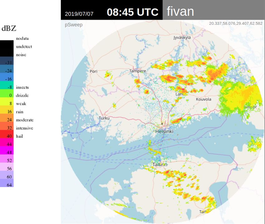
Acronyms

Cb: Cumulonimbus

FMI: Finnish Meteorological Institute

TCU: Towering cumulus

METAR: METeorological Aerodrome Report

CIN: convective inhibition

CAPE: convective available potential energy

LFC: level of free convection

EL: equilibrium level

ICAO: International Civil Aviation Organization

ARP: aerodrome reference point

PRF: pulse repetition frequency

FAR: False Alarm Ratio

POD: Probability of Detection

CSI: Critical Success Index

                                          3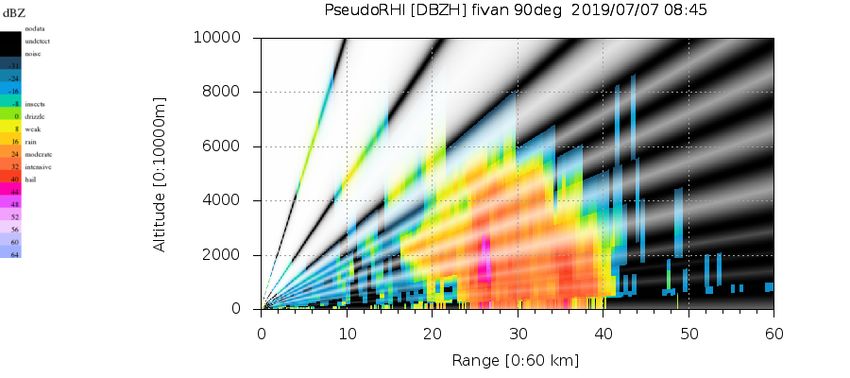
1. Introduction

Cumulonimbus (Cb) clouds are a serious threat to aviation as they can produce hazardous
weather such as turbulence, icing, lightning, wind shears, micro-bursts, hail and intense
precipitation (International Civil Aviation Organization, 2018). These severe weather
hazards associated with Cb clouds increase the annual costs of the aviation industry
due to the increased time and lost fuel, as some flights might be delayed, cancelled or
rerouted. For all of the above reasons, it is important to forecast, detect and monitor Cb
clouds as well as possible. Therefore, it is also relevant to understand convection since it
initiates Cb clouds.

Finnish Meteorological Institute (FMI) is responsible for providing aeronautical
meteorological services in Finland (Finnish Meteorological Institute, 2020b). This
includes doing the METeorological Aerodrome Report (METAR), which describes the
weather at the aerodrome and its vicinity. At Helsinki-Vantaa airport (EFHK) METARs
are done by a human observer around the clock all year round. At all other Finnish
airports, METARs are at least partially done automatically. Automatic METAR is
called AUTO METAR. Since significant weather is reported in METAR, also towering
cumulus and Cb clouds must be included. On METARs done manually by an observer,
Cb detection is primarily based on the observer’s observations on the shape and the
height of the cloud (Nikkanen, 2020). Sometimes, Cb detection conditions can be more
difficult, for example, when it is dark or if the Cb cloud is embedded in the cloud layer.
In addition, having human observers working around the clock all year around is costly.
Therefore, automation of Cb detection is a topical matter.

Also other countries are interested in automatic Cb detection in Europe. For ex-
ample, a system that is using both radar and satellite observations is used in the
Netherlands (De Valk & van Westrhenen, 2015). In addition, a similar system is applied
in Germany (Kober & Tafferner, 2009). According to Honorè et al. (2010), France
operates a system that uses lightning and weather radar observations to detect Cb
clouds. Automated Cb detection systems are not only used in Europe but around
the world. For example, they are nowadays applied at some airports in Japan (Japan

                                             4
5 Chapter 1. Introduction Meteorological Agency, 2016) and in New Zealand (Hartley & Quayle, 2014). FMI is likewise applying an algorithm that uses observations from weather radars to detect Cb clouds (Hyvärinen et al., 2015). Information of Cb clouds has been in AUTO METARs from years 2018-2019 (Nikkanen, 2020). Also, human observers can utilise it when detecting Cb clouds. It is reasonable to study how well this scheme can detect Cb clouds and what could be done to improve it. The operation of the algorithm is based on the ability of the weather radar to detect precipitation. Precipitation is detected with a value called a radar reflectivity factor. The aim of this thesis is to examine how well FMI’s algorithm can detect Cb clouds compared to manual observations. Summer months are studied as Cb clouds are more common and stronger in Finland then due to more unstable atmosphere (Eastman & Warren, 2014). The reasons for differences are discussed, and furthermore, improvements for the algorithm are suggested. A hypothesis is that the weather radar observations and the algorithm, when it is working properly, could be better than human observations in most cases. Therefore, the algorithm could be the only tool that is used to detect Cb clouds for both manual and automatic METARs in the future. In the next chapter, Chapter 2, some theory and background information, which helps to understand the later study, will be discussed. Then, Cb clouds and METARs are explained in more detail. In addition, the basics of radar meteorology and radar geometry are considered. After the theory chapter, data and methods used in this thesis are described in Chapter 3. In the following Chapter 4, the results of this thesis are processed and reviewed. Furthermore, some case examples are introduced to deepen understanding of differences and similarities between human observation and algorithm detection. Also, possible future steps are introduced and discussed. Finally, conclusions are drawn in Chapter 5.
2. Theory

2.1. Convection
Convection is transport of heat, momentum and moisture due to the movement of fluid
in the atmosphere. Conceptually, convection transfers warm air upward and cold air
downward. Heat can be either sensible or latent. Latent heat is related to a substance
changing its physical state, for example, when water vapour is condensed into liquid
water droplets. If no clouds are formed by convection, the convection is called dry.
When phase changes of water have an essential role in convection and clouds are formed,
the convection is called moist (Emanuel, 1997). Nevertheless, both types of convection
remove excessive heat from the surface and transport it into the atmosphere. When
the vertical motions extend from the lower atmosphere above 500 hPa, convection is
referred to as deep (Davidson, 1999). So before discussing Cumulonimbus (Cb) clouds, it
is important to understand deep moist convection, which is responsible for Cb and other
cumulus cloud development (Markowski & Richardson, 2010). In this thesis, deep moist
convection is referred to as convection.

Two requirements need to be fulfilled so that convection can initiate (Markowski
& Richardson, 2010). The first one is that air needs to reach its level of free convection
(LFC). This typically means that air needs some forced ascent to get there since some
amount of convective inhibition (CIN) is usually present. CIN is the amount of energy
that will prevent an air parcel from rising from the surface to LFC (Markowski &
Richardson, 2010). It can be written as
                                             Z LF C
                                  CIN = −             Bdz                            (2.1)
                                                0

where B is the buoyancy force. B is integrated from the surface to the LFC. CIN is
negative because it is the work that must be done to lift an air parcel to LFC.

From LFC, an air parcel can freely accelerate upward as it becomes buoyant rela-
tive to its environment (Holton & Hakim, 2012). The second requirement is that the air

                                            6
7 Chapter 2. Theory
parcel should have convective available potential energy (CAPE), which means that after
reaching LFC, the air parcel must remain positively buoyant in a deep enough layer.
CAPE can be written as Z EL
CAP E = Bdz (2.2)
LF C
where B is the buoyancy force. B is integrated from LFC to the equilibrium level (EL).
At the EL, the air parcel has become equal to the temperature of the surrounding air.
Above the EL, the air parcel becomes negatively buoyant and convection stops. However,
the air parcel might continue to rise after EL because it still has some kinetic energy left
at EL. The Equation 2.2 tells that CAPE is equal to the amount of work done by the
buoyancy force. Figure 2.1 below illustrates an example of a sounding. CIN, CAPE, LFC
and EL are also marked in Figure 2.1 where the light blue area is CIN, and the orange
area is CAPE.
Figure 2.1: Example of a sounding. CIN = light blue area, CAPE = orange area. LFC (as LF CT ) and
EL are marked in the figure.
Since large CAPE values are needed for convection to initiate, conditions when it happens
need to be understood. Large CAPE values are possible when temperature lapse rate
in lower and middle troposphere is at least larger than moist adiabatic lapse rate Γs
(Markowski & Richardson, 2010). That way lifted air parcel will cool down slower than
its environment. Temperature lapse rate is large when the boundary layer is warm and
moist and the free troposphere is cold. The lapse rate tendency equation 2.3 tells how
the temperature lapse rate can change and thus initiate convection:
∂γ ∂γ ∂vh ∂w 1 ∂q
= − vh · ∇h γ − w + · ∇h T + (Γd − γ) − . (2.3)
∂t ∂z ∂z ∂z cp ∂z
| {z }| {z }| {z }| {z } | {z }
I II III IV V8 Chapter 2. Theory
Term I represents horizontal and term II vertical lapse rate advection. Term III is
differential temperature advection when it is combined with the first term. Term IV
is called a stretching term. The last term V is diabatic heating. vh is the horizontal
wind velocity, w is the vertical wind velocity, Γd is the dry adiabatic lapse rate, cp is
the specific heat at constant pressure and q heating rate. The derivation of the above
Equation 2.3 is not shown in this thesis since it is unnecessary. It is here only to show
what factors have an effect on lapse rate tendency.
Next, a simple example of how lapse rate can change to initiate convection is pre-
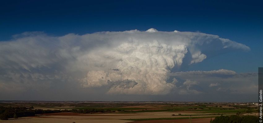
sented. In this example, term V from Equation 2.3 is changed to modify lapse rate.
When diabatic heating is decreased with height, it means that the differential ∂z ∂q
is
negative. Since the specific heat at constant pressure cp is a positive constant, the lapse
rate is increased in time ( ∂γ
∂t
> 0). Similarly, when diabatic heating is increased with
height, the lapse rate is decreased. This example is shown in Figure 2.2, where above the
maximum heating level (z1 ) lapse rate is increased and below decreased.
Figure 2.2: Example of how differential diabatic heating can change lapse rate.
There are also other ways that can change CAPE and CIN without changing the lapse
rate. For example, CIN can be reduced by low-level moistening or warming (Markowski &
Richardson, 2010). Especially low-level moistening is independent of lapse rate changes.
Low-level warming and deepening of the low-level atmosphere are common when the Sun9 Chapter 2. Theory
is rising. That leads to decreased CIN, which makes convection initiation easier. Note
that both low-level warming and moistening also have a positive effect on CAPE. Another
way to change CIN and CAPE without changing lapse rate is through a large scale ascent
(Markowski & Richardson, 2010). That is because the mean ascent is associated with
adiabatic cooling that leads to reduced CIN.
2.2. Cumulonimbus cloud
Clouds can be classified according to their shape and height. There are three different
classes for the height classification: the bases of the low-level clouds are from 0 to 2 km, the
bases of the middle-level clouds are from 2 to 7 km, and the bases of the high-level clouds
are from 5 to 13 km (Karttunen et al., 2001). Cumulonimbus1 (Cb) clouds are classified as
low-level clouds, yet they can still extend to all three height levels (Karttunen et al., 2001).
According to World Meteorological Organization (2017), a Cb cloud is an optically
dense cloud with a significant vertical extent, which is approximately ten kilometres, and
it is formed by convection. Its upper part is almost always flattened, it spreads out like
an anvil and is usually smoothened, fibrous or striated. The base of the cloud is often
dark, and there are usually low, ragged clouds. Picture 2.3 below is a good example of a
Cb cloud.
Figure 2.3: Cumulonimbus cloud. (World Meteorological Organization, 2017)
There is always rain in a Cb cloud, and the rain is of showery type. A Cb cloud can also
produce lightning, thunder and hail. A Cb cloud can initiate from different cloud types,
i.e. from Cumulus congestus, Altocumulus castellanus, Stratocumulus castellanus, or it
can also be embedded in Altostratus or Nimbostratus (World Meteorological Organiza-
1
Cumulus is a Latin word meaning heaped and nimbus rainstorm.10 Chapter 2. Theory
tion, 2017). Because a Cb cloud forms most commonly from Cumulus congestus, it is
sometimes difficult to distinguish them. The cloud is identified as Cb when its upper
part loses its sharpness or presents a fibrous or striated texture (World Meteorological
Organization, 2017).
Cb clouds can be isolated, appear in clusters or along fronts. Duration of one sin-
gle cell is usually about 0.5 − 2 hours, and the diameter can be from 500 metres up to
20 kilometres (Karttunen et al., 2001). Single-cell convection is next considered. There
are three different stages of a storm in single-cell convection: towering cumulus stage,
mature stage and dissipating stage. These different stages are illustrated in Figure 2.4.
Towering cumulus stage is a stage where there is only an updraft, and the lifecycle of an
ordinary cell begins with this stage. The anvil starts to form in the mature stage, and
the water droplets in this stage are large enough to fall through the updraft. The falling
precipitation and the evaporation of precipitation induce a downdraft. The gust front at
the ground is formed to the leading edge of the downdraft. There is heavy precipitation
and, additionally, lightning is possible in the mature stage. The dissipating stage begins
when the downdraft dominates the cell, and the updraft cannot be maintained. Now,
new cells can be initiated by the gust front. Initiation depends on CIN and vertical
motions in the gust front. Figure 2.4 visualises the three different stages in single-cell
convection.
Figure 2.4: Schematic figure of three stages of an ordinary convective cell.
Multicellular convection consists of multiple single-cells where each cell is in the different11 Chapter 2. Theory
stage, and the new single-cells are repeatedly generated by the gust front (Markowski &
Richardson, 2010). Multicellular convection is the most common type of convection in
the mid-latitudes. If the circumstances in the atmosphere are favourable, supercellular
convection may be initiated. Supercells can last up to 9 hours but are very rare in
Finland, so they are not studied in detail (Karttunen et al., 2001).
Cb clouds appear in Finland mostly in summer when unstable lower troposphere
is more common than in winter (Karttunen et al., 2001). That is why a dataset from
the summer months is used in this thesis. However, they can still form in winter, for
example, over the Gulf of Finland if the sea surface is unfrozen. Vertical extent of cb
clouds in winter is lower as the troposphere is colder, more stable and the tropopause is
lower (Karttunen et al., 2001).
2.3. METAR
Finnish Meteorological Institute (FMI) is responsible for providing aeronautical me-
teorological services for civil and military users in Finland (Finnish Meteorological
Institute, 2020b). METeorological Aerodrome Report (METAR) is one of the services
that FMI provides. METAR is a local routine observation report that describes the
weather at the aerodrome or its vicinity (International Civil Aviation Organization, 2018).
METARs are regulated by the International Civil Aviation Organization (ICAO)
and EU. ICAO and EU define the content, format and release time of the METARs
(International Civil Aviation Organization, 2018). ICAO regulates that METAR report
must contain the following information:
• location indicator
• observation time
• surface wind direction and speed
• visibility
• runway visual range (when applicable)
• present weather
• cloud amount
• cloud type (only if the cloud is towering cumulus (TCU) or cumulonimbus type)
• height of the cloud base (or vertical visibility where measured)
• air temperature
• dew-point temperature
• the atmospheric pressure (QNH/QFE).12 Chapter 2. Theory METARs are primarily used by aircraft pilots who use it for the flight planning and meteorologists who use it for the weather forecasting among other products. In Finland METAR observations are done every 20 and 50 minutes past the hour. Only the operationally significant weather is reported in METAR, and according to the ICAO regulations, clouds and other remarkable weather phenomena are observed within a maximum radius of 16 kilometres from the aerodrome reference point (ARP) (International Civil Aviation Organization, 2018). ARP is the geographical location of an aerodrome. METARs can be done manually by human or automatically. If the METAR is done automatically, it is specified in the head of the METAR af- ter the time group with the word AUTO. Helsinki-Vantaa airport is the only airport in Finland where METARs are done by a human observer around the clock all year round. Clouds at the aerodrome or its vicinity (maximum radius of 16 km from the ARP) are reported in METAR if they are operationally significant (International Civil Aviation Organization, 2018). This means that clouds with a base under 1500 metres (5000 feet) or TCU or Cb clouds are reported. In reality, a human observer observes significant clouds over the 16 kilometres radius (Isolähteenmäki, 2020). Usually, this happens if the observer thinks that it is important to air traffic: for instance, if Cb cloud is near the runway. An observer can identify Cb cloud based on the shape and height of the cloud. This information is discussed in the previous section in more detail, but the cloud can be identified as Cb if its vertical extent is large, the upper part of the cloud spreads out like an anvil, and the outline of the cloud top is not as sharp as in a TCU. In addition, if the cloud base is very dark, the cloud is usually identified as Cb, even if the cloud is embedded in the cloud layer, and the cloud top is not visible (Tikkamäki, 2020). A clear indication of Cb cloud is thunder, lightning or both. Also, if the precipitation is of a showery type or in the form of virga, it can be classified as Cb cloud. Cb clouds can be identified manually with the help of ceilometers. Ceilometers determine the height of a cloud base by using a laser or other light source. There are several ceilometers at Helsinki-Vantaa, which are used especially when determining the height of the cloud base or vertical visibility (Finnish Meteorological Institute, 2020b). In addition, an observer can use radar observations to determine whether the cloud is Cb. In some cases, manual Cb detection can be better than automatic detection since the observer is often aware of the meteorological situation and can utilise his/her expertise to detect the Cb cloud even when it is not visible (International Civil Aviation
13                                                                 Chapter 2. Theory

Organization, 2018). On the other hand, the manual Cb detection can be difficult if
it is dark or when the Cb cloud is buried in clouds and the cloud tops are not visible
(EMBD CB situation). For example, Cb clouds can be obscured by other low clouds in a
frontal system. In these cases, the automatic Cb detection algorithm can be better than
human. In addition, also other reasons support automatic Cb detection; measurements
are objective and it also saves money not to have staff working in shifts. Therefore, the
automatic algorithm that can detect Cb clouds with a sufficient accuracy could be the
choice of the future in Finland. Later in this thesis, it is studied how accurately the
algorithm detected Cb clouds compared to the manual observations in the summers of
2016-2020.

2.4. Weather radar geometry
Radars are used in a wide variety of applications. In this section, the focus is on weather
radars that can be used to observe the atmosphere. The weather radars operate in
microwave frequency range since the microwaves can reveal the inner structure of intense
storms and Cb clouds (Rauber & Nesbitt, 2018). This is a major advantage of radar Cb
detection because an observer cannot see the inner structure of a cloud. Radars at FMI
have a wavelength of 5.3 centimetres which means these are C-band radars (Saltikoff
et al., 2010).

The antenna of the weather radar sends high powered microwave pulses in differ-
ent directions. When the pulse encounters a target, part of its power is reflected and
scattered back to the antenna (Rauber & Nesbitt, 2018). Subsequently, the weather radar
receiver measures the power of the reflected pulse and its travel time. The former tells
the intensity of precipitation, and the latter tells the distance of the obstacle from the
radar. The more intense precipitation, the stronger the echo is. Weather radars cannot
detect convective clouds before water vapour is condensed into liquid water droplets.
They are very sensitive devices, as the power of the reflected pulse is only a tiny fraction
of the total transmitted power. To illustrate this, the transmitted power can typically be
250 000 watts, and the reflected power can be only from 1 · 10−6 to 1 · 10−7 watts.

FMI’s weather radar in Vantaa, Kaivoksela is used in this thesis because it is
close to Helsinki-Vantaa airport where METARs are reported. Technically, the data is
from a composite that covers the whole Finland, but as the radar in Vantaa is closest to
Helsinki-Vantaa airport, and there are no other radars in the vicinity, the radar in Vantaa
is the one which has taken the measurements needed in this thesis. The model of the
radar is WRM200, and it is manufactured by Vaisala. WRM200 is a dual-polarization
14                                                                 Chapter 2. Theory

Doppler radar. In order to understand the Cb detection algorithm, it is essential to
understand the basics of radar measurement geometry. Measurements on a daily basis
are carried out as elevation scans. This means that with each scan the circular antenna
rotates 360 degrees with a constant elevation angle. From this, one conical surface is
produced. The measurements consist of several elevation scans which produce a set of
nesting conical surfaces. This dataset is called a volume scan. A volume scan is done
every five minutes, although the specific elevation angles used in a volume scan vary
slightly depending on the time (Finnish Meteorological Institute, 2020c). For instance,
hh:00-hh:05 scan uses 13 different elevation angles, whereas hh:05-hh:10 scan uses nine
different elevation angles. In Figure 2.5 below, the volume scan is illustrated.

                      Figure 2.5: Volume scan. Figure by Markus Peura.

Cb detection with the weather radar is based on the quantity called a radar reflectivity
factor Z(dBZ) which is called as a radar reflectivity in common usage (Rauber & Nesbitt,
2018). The radar reflectivity factor is probably the most important quantity in radar
meteorology. The radar reflectivity factor is related to the power that is returned back to
the weather radar by the weather radar equation. It can be calculated as
                                                Dj6
                                             P
                                               j
                                       Z=                                             (2.4)
                                               Vc

where D is a diameter of hydrometeor and Vc is a unit volume. Subscript j represents
that summation is carried out over all scattering targets. Note, that in this Equation
2.4, it is assumed that the Rayleigh assumption is valid. This means that hydrometeors
are small compared to the wavelength of the radar (Rauber & Nesbitt, 2018). With
a C-band radar, this assumption is not valid if the size of hydrometeor is larger than
approximately 2 centimetres which means that the type of the hydrometeor is hail. In
addition, hydrometeors must be spherical. This condition is only met by small raindrops,
some frozen raindrops and some graupel and hail (Rauber & Nesbitt, 2018). However,
Rayleigh scattering is usually assumed, although it is unlikely to be met in many cases.
15 Chapter 2. Theory
When it is obvious that the Rayleigh criteria cannot be assumed, the term equivalent
radar reflectivity factor can be used (Rauber & Nesbitt, 2018). In this thesis, it is not
discussed in more detail because it is irrelevant for the basics of the radar measurements.
Although the radar receives power that was scattered back to radar, it does not tell
anything alone. In practice, the radar reflectivity factor is needed since a parameter that
is more directly linked to the physical properties of the precipitation is wanted. When
the reflectivity factor is of a certain size, the target can be classified as a Cb.
The algorithm which FMI is using is adopted from Météo-France (Leroy, 2006).
Radar takes measurements every five minutes, which means the Cb cloud analysis is
done equally often. It is done by investigating the vertical structure of reflectivities from
radial resolution data (Hohti, 2020). In the beginning, individual points and radial lines
that are considered as clutter are cleaned from the polar data. It is then investigated if
the reflectivity threshold values are exceeded in a sufficient number of different heights.
According to Leroy (2006), France is using the following reflectivity threshold values for
Cb: lower threshold value is 33 dBZ, and the upper one is 41 dBZ. In addition to the
definition by Leroy (2006), there are some additional criteria at FMI that need to be
fulfilled for the reflection to be classified as a Cb cloud (Hohti, 2020):
• these threshold values are implemented to a vertical column of a polar volume
• the reflectivity factor should exceed the lower threshold value for at least in two
elevation angles
• the reflectivity factor should exceed the upper threshold value at least in one eleva-
tion angle
• these threshold values are decreased a few dBZ as a function of distance, as smooth-
ing of small phenomena increases when the distance from the radar increases
• the reflectivity must be consistent in a vertical direction: gaps, where the radar
reflectivity factor drops below 5 dBZ, are not allowed
• to avoid ground clutter, measurements are accepted approximately only above 200
metres.
When all the aforementioned conditions are met, the target is classified as Cb. A
graphical explanation of what the reflection could look like when a weather radar
observes Cb is in Figure 2.6 below.16 Chapter 2. Theory
Figure 2.6: Example of Cb observed by radar. Colours describe the reflectivity factor. Red: 33 dBZ <
Z < 41 dBZ. Purple: Z > 41 dBZ.
Next, a real vertical cross-section of Cb and the related radar reflectivity factor is in-
troduced. This is illustrated in Figure 2.7, which is a pseudo-range-height indicator
(pseudo-RHI) image. This means that the image is interpolated from a 3D volume con-
sisting of several azimuthal scans. It can be seen that the radar reflectivity factor is at its
greatest about 44 dBZ in the middle of a Cb cloud. This fulfils the upper threshold value
(Z > 41dBZ) at least in one elevation angle. The lower threshold value (Z > 33dBZ) is
also fulfilled at least in two elevation angles. Thus, the reflection in Figure 2.7 is clearly
classified as a Cb.
Figure 2.7: Pseudo-RHI image of Cb.
This situation in Figure 2.7 can be seen in Figure 2.8 as a plan position indicator (PPI)
image. The pseudo-RHI image in Figure 2.7 is a cross-section to the east from the Vantaa
radar. The small black cross in Figure 2.8 represents approximately the location of the
radar.17 Chapter 2. Theory
Figure 2.8: PPI image of Cb.
Since the weather radars at FMI are dual-polarization radars, their measurements
contain some additional variables. That is due to dual-polarization radars transmit
and receive pulses in both vertical and horizontal direction (Rauber & Nesbitt, 2018).
As a result, they give more information about the size and shape of the targets. For
instance, one of these variables is called differential reflectivity ZDR (Rauber & Nesbitt,
2018). Differential reflectivity is the difference between horizontal reflectivity and vertical
reflectivity: ZDR = ZH − ZV and it can help to identificate hydrometeors (Woodard
et al., 2012). Also, two other variables, the correlation coefficient ρHV and the specific
differential phase KDP can be used in identifying hydrometeors. The identification of
hydrometeors is important since the type of hydrometeor can tell about the presence of
Cb clouds. For instance, supercooled raindrops above the freezing level have predicted
lightning to occur (Woodard et al., 2012).
Effective measurement range of the radar depends on the weather. Theoretically,
with the setup used at FMI, the measurement range of the weather radar can be up to18 Chapter 2. Theory
250 kilometres. This maximum range is defined as
c
rmax = (2.5)
2(P RF )
where c is the speed of light and PRF is the pulse repetition frequency (Rauber & Nesbitt,
2018). PRF depends on the type of radar, but it is usually 100-1000 times in a second.
Targets that radar is observing must be within rmax . The PRF is approximately 570 per
second at FMI (Saltikoff et al., 2010), so rmax can be calculated as
299792458m/s
rmax = = 262975.84035...m ≈ 250km. (2.6)
2 ∗ 570Hz
However, e.g. snowfall in winter can be detected with a maximum range of 120 kilometres.
One reason for this is that clouds are lower in winter and therefore below the radar beam
(Karttunen et al., 2001). In addition, the curvature of the earth limits echoes of targets
to be within rmax : if a target is beyond rmax , it is likely to be below the radar beam and
radar cannot detect it (Rauber & Nesbitt, 2018).3. Data and methods
This chapter discusses in more detail the data used and how it is processed in this thesis.
In addition, different kinds of verification scores are introduced.
A dataset that contains the summer months from 2016 to 2020 is used in this
thesis. June, July and August are considered as summer months. The radar dataset is
compared with METARs since it is considered that METARs give the best information
about the presence of Cb clouds at Helsinki-Vantaa airport and its vicinity. METARs are
sent every 20 and 50 minutes past the hour, and the observation time for the METAR is
ten minutes before it needs to be sent (Finnish Meteorological Institute, 2020a). Weather
radars make one full volume scan every 5 minutes in Finland. Because the METARs and
the radar measurements have a different schedule, they need to be matched together.
There are two ways this can be done. The first option is to use the radar data from 20
and 50 minutes past the hour because that time is as close as possible with the time
that METAR needs to be sent. The second option is to use the radar data from both 15
and 20 minutes past the hour and 45 and 50 minutes past the hour to cover the whole
ten-minute METAR observation period. Both options are considered and compared,
which one of the methods would be better in this thesis.
After pairing these two observation sources, differences between the Cb detection
algorithm and human-based METAR observations are analysed. In total, the dataset
contains 22048 METAR observations. This means there are 32 METARs missing since
theoretically there should be 22080 METARs from that specific time period. From the
22048 METARs, there are 2266 METARs where Cb was observed, and 19782 METARs
where Cb was not observed. Furthermore, it is studied how many cases there are where
both the algorithm and human observations did not detect a Cb cloud. Various di-
chotomous verification scores are calculated for the radar-METAR Cb observation-pairs.
Finally, it is discussed what caused the disagreements between detection of the algorithm
and observer’s observations.
After the whole dataset is studied, it is divided into two groups: one for daytime
1920 Chapter 3. Data and methods observations and the other one for night-time observations. The daytime is specified to be between 6 UTC − 18 UTC, and the night-time between 18 UTC − 6 UTC as the same hours are used in some SYNOP measurements. Note, that in summer there is dark approximately only five to nine hours per night. The difference between the night-time and daytime Cb detection accuracy is studied. Then, it is studied if there are any differences in the detection accuracy between different years or months. First, different verification scores are calculated individually to each year and compared together. After that, the dataset is grouped by month, and similarly what was done to different years, verification scores are calculated to each month and compared with each other. It was mentioned before in Chapter 2 that the range of weather radars can be even 250 kilometres in good weather. In the algorithm, such long range is not necessary since ICAO standards regulate that Cb clouds have to be detected at the aerodrome and its vicinity (International Civil Aviation Organization, 2018). Therefore, the range in the Cb detection algorithm is specified to be 20 kilometres. Similarly, the observer at the airport is only detecting Cb clouds in the range of approximately 16 kilometres. The algorithm uses a larger range because sometimes the observer’s detection range can be a bit over 16 kilometres. The radar in Vantaa is close to Helsinki-Vantaa airport. A starting point to Cb detection with weather radars is the polar data (ODIM HDF5 format) (Finnish Meteorological Institute, 2020c). The algorithm was described in more detail in Chapter 2, so it is not repeated here. The detection algorithm has been pre-operative at FMI since 2011 and meteorologists have been using it among other tools, especially under challenging conditions. These difficult conditions include darkness or embedded Cb, for example. 3.1. Validation Cb cloud detection can be regarded as a dichotomous event, and therefore it can be referred to as yes/no events. The possible outcomes can be presented in a contingency table where all the possible outcomes of an event are shown (Jolliffe & Stephenson, 2012). In this study, the contingency table has a shape of 2x2. The contingency Table 3.1 can be used to determine numerous verification scores (Wilks, 2011). Different verification scores can tell about the accuracies of the results, and they can be calculated from the number of hits, false alarms, misses and correct negatives.
21                                                       Chapter 3. Data and methods

Hits are the cases when both the algorithm and the observer detected a Cb cloud. Misses
mean the cases where the observer detected a Cb cloud, but the algorithm did not. On
the contrary, false alarms mean the cases where the algorithm detected a Cb cloud, but
the observer did not. Note, it does not necessarily mean that the algorithm was wrong:
it can also be a case when the observer could not see a Cb cloud. However, human-based
observations are used as the ground truth in this study, so that is why these kinds of
cases are called false alarms. Correct negatives are the cases when both the algorithm
and the observer did not detect a Cb cloud. Not all scores mentioned below are used to
measure the accuracy but some other value, for instance, over- or underdetecting of Cb
clouds.

                                       Observed 1        Observed 0
                        Detected 1         Hits          False alarms
                        Detected 0       Misses       Correct negatives

                          Table 3.1: A contingency table. (Wilks, 2011)

From the contingency table 3.1, several different verification scores can be calculated.
In this thesis, the False Alarm Ratio (FAR), the Probability of Detection (POD), the
Critical Success Index (CSI) and the bias are used to analyse the results.

The FAR is the fraction of the detections where a yes-event was detected but not
observed (Wilks, 2011). False Alarm Ratio is calculated instead of False Alarm Rate
( F alse alarms+Correct
            F alse alarms
                          negatives
                                    ) because the occurrence of Cb clouds is a rare event and thus
False Alarm Rate could become misleadingly low when the number of correct negatives
is high. In this thesis, an observed yes-event is an event when an observer observed a
Cb cloud. Likewise, a detected yes-event is an event when the algorithm detected a Cb
cloud. So, FAR is the fraction of the cases when the algorithm detected a Cb cloud but
the observer did not. The FAR can have values from 0 to 1. The smaller the FAR is, the
better Cb detection with the algorithm is. In other words, if the FAR is 0, the detection
was always also observed. FAR tells about the reliability of the scores. FAR can be
calculated as the following:
                                            F alse alarms
                               F AR =                         .
                                         Hits + F alse alarms
The POD is the ratio of observations where yes-event was both detected and observed to
the number of detections where yes-event was both observed and detected (hits) or only
observed (misses) (Wilks, 2011). In this study, it means that POD is the cases where
both the algorithm and the observer observed a Cb cloud divided by the number of times
a Cb cloud was observed. The POD can have values from 0 to 1, but unlike with FAR, 1
22 Chapter 3. Data and methods
is the best score for the POD. POD can be calculated as:
Hits
P OD = .
Hits + M isses
The CSI (also called as the threat score) is the correct forecasts (hits) divided by the total
number of detections where yes-event was detected, observed or both (Wilks, 2011). It
can have values from 0 to 1. The bigger the CSI value is, the more accurate Cb detection
with the algorithm is. CSI describes the accuracy well with low-frequency events since
the correct negatives are not considered (Jolliffe & Stephenson, 2012). Cb clouds can be
considered as rare events according to the numbers in the contingency table. According
to Jolliffe & Stephenson (2012), CSI would not be suitable even for rare events because it
tends to a limit of zero when observed events are close to zero. However, this is not the
case in this study, so CSI can be used. CSI can be calculated as the following:
Hits
CSI = .
Hits + M isses + F alse alarms
The bias is a ratio of the number of detections to the number of observations (Wilks,
2011). In this thesis, it means that it is a ratio between the detected Cb clouds by the
algorithm and the observed Cb clouds by the observer. If bias is equal to one, it means
that the number of times the event was forecasted and observed were equal. If the bias
is under one, it means underdetecting and if it is over one, it means overwarning of the
detected yes-events. Bias is not used to analyse the accuracy of the results but to tell if
the event is classified more or less than observed. The desired value for bias depends on
the user and the event of interest (Jolliffe & Stephenson, 2012). In this study, if the bias
were equal to one, Cb clouds were detected as many times as observed. This would be
optimal for the study. Bias can be calculated as the following:
Hits + F alse alarms
BIAS = .
Hits + M isses
All in all, FAR and POD tell about the reliability of the detection, but neither one of
the measures are suitable on its own (Jolliffe & Stephenson, 2012). As a rule of thumb,
the bigger the POD and the smaller the FAR, the better the algorithm is at detecting
Cb clouds. However, when FAR is decreased, it yields to decreased POD. Similarly,
increased FAR yields to increased POD. In this thesis, POD is prioritised over FAR,
which means that increased FAR is accepted as misses and underdetection of Cb clouds
are more dangerous to aviation than false alarms and overdetection. CSI tells about the
detection accuracy, and it works well with low-frequency events. The bias tells about
over- or underforecasting.4. Results
The dataset consists of the summer months from 2016 to 2020. Summer months are
defined to be from June to August. The values that are measured 20 and 50 minutes
past the hour are chosen from the weather radar data. Next, the METAR dataset is
combined with the weather radar dataset and the verification scores are calculated from
the combined dataset.
In total, there are 1272 cases where Cb is detected by both human observer and
weather radar. There are 994 cases where human observer has detected Cb but weather
radar has not. On the contrary, there are 414 cases where weather radar detected
Cb but human observer did not. Lastly, there are 19367 cases where neither human
observer nor weather radar detected Cb. These aforementioned values are represented in
a contingency table in Table 4.1 below.
Observed 1 Observed 0
Detected 1 1272 414
Detected 0 994 19367
Table 4.1: The contingency table of the scores.
Subsequently, FAR, POD, CSI and bias can be calculated from Table 4.1. The theory
behind the verification scores can be found in Chapter 3. As a result, the FAR is
equal to 0.25, the POD is equal to 0.56, the CSI is 0.47 and the bias is 0.74. Value of
bias states that the radar underdetected Cb clouds compared to human observations.
This underdetecting is considered to be dangerous to aviation, but it is important to
understand that human observers can observe Cb clouds overeagerly and from a bigger
radius. Therefore, the result is not as reliable. The POD being 0.56 means that over half
of the observed Cb clouds were detected by the algorithm.
The measurements taken 15 and 45 minutes past the hour from the radar data
can be included in the calculations. This is done because the observation time for
METAR is the past 10 minutes before it needs to be sent. Consequently, the values of 15
2324 Chapter 4. Results
and 45 minutes past the hour are taken into account to see if they have any impact on
the accuracy of the results. Cb is considered to be detected if there is Cb in either one
of the minutes 15 or 20 and 45 or 50 past the hour. The results are represented in Table
4.2.
Observed 1 Observed 0
Detected 1 1363 515
Detected 0 903 19266
Table 4.2: The contingency table of the scores when 15 and 45 minutes past the hour are taken into
account.
When the consecutive radar measurements are considered, there are more cases where
both the algorithm and observer detected Cb and more cases when only a radar detected
Cb. This can be seen from Table 4.2 above. On the other hand, there are fewer cases
when only a human observed Cb. FAR, POD, CSI and bias can be calculated from the
contingency table 4.2. The FAR is equal to 0.27, the POD is equal to 0.60, the CSI
is equal to 0.49 and the bias is equal to 0.83. Compared to the first results, FAR is
worse, but POD, CSI and bias are better. As was stated in Chapter 3, increased POD is
preferred over decreased FAR; therefore, this result is here considered better than the first
one. CSI is also higher, which states that the accuracy of the result is better. The bias
is closer to one, which means that underdetecting is not as strong as in the first calculation.
Overall, both the 15 and 20 minutes as well as 45 and 50 minutes past the hour
measurements are taken into account in the following calculations since it seems to
describe the situation better and give better accuracy of the results. According to Henken
et al. (2009), POD is required to be over 0.8 and FAR under 0.2 in order to replace
human observers by an automated system in the Netherlands. If these same threshold
values were implemented in Finland, the FAR of 0.27 and the POD of 0.60 would not be
sufficient enough, and the algorithm as such could not yet replace human observers at
Helsinki-Vantaa.
Next, the data are divided into daytime and night-time. The daytime is defined
to be from 6 UTC to 18 UTC, and the night-time to be from 18 UTC to 6 UTC. These
hours are selected because the SYNOP observations are also done then, and hours from
6 UTC to 18 UTC (local time from 09:00 to 21:00) describe the daytime convection the
best. In the daytime dataset, there are total of 1678 METAR observations where Cb
was observed, and 9348 METAR observations where Cb was not observed. Likewise,
there are 588 METAR observations at the night-time, where Cb was observed, and 1043425 Chapter 4. Results
METAR observations where Cb was not observed. Then, similarly to what was done
to the whole dataset, METAR observations are combined with the radar dataset. The
results are illustrated in Table 4.3.
Daytime Night-time
Cb was observed by human and radar 996 367
Cb was observed only by human 682 221
Cb was observed only by radar 257 258
Cb was not observed by human or radar 9091 10175
Sum 11026 11021
Table 4.3: Values for separate daytime and night-time detections.
It can be seen from Table 4.3 that there is in total almost the same number of observations
in both groups, 11026 values for daytime and 11021 values for night-time. However,
there are more cases in the daytime when only a human observer has detected Cb and
more cases where both the observer and the weather radar have observed a Cb cloud. In
general, there are more Cb clouds in the daytime, because the Sun warms the atmosphere
and thus destabilizes the boundary layer and initiates convection (Eastman & Warren,
2014).
The diurnal cycle can also be seen in Figure 4.1 below, where Cb observations of
each day are summed up and divided into different hours of the day. This is done to both
METAR observations as well as radar detections. Figure 4.1 illustrates the same thing
that was previously concluded from Table 4.3: there are more Cb clouds in METARs in
the daytime and in contrary, more Cb clouds are detected by radar in the night-time.
At 06 UTC (09:00 local time), both the radar and human observers observed the same
amount of Cb clouds. Note that the hours in Figure 4.1 are UTC (in Finland the time
is three hours ahead from UTC). Figure 4.1 shows that most of the Cb clouds are in the
daytime, more specifically in the afternoon (highest peaks at 11 UTC, 14:00 local time
and 12 UTC, 15:00 local time). In addition, a human observer may prefer to overobserve
Cb clouds since it is less dangerous to aviation than underobserving. It is also possible
that human observers have observed Cb clouds much further away than 16 kilometres
from the ARP since sometimes Cb clouds can appear to be closer than they are in reality
(Nikkanen, 2020). In the night-time, overobserving of Cb clouds is more difficult since it
is dark.26 Chapter 4. Results
Figure 4.1: Cb observations per hour.
Next, the contingency tables can be separately created for both night-time and daytime
detections. These values are in Table 4.4.
Daytime Night-time
Observed 1 Observed 0 Observed 1 Observed 0
Detected 1 996 257 Detected 1 367 258
Detected 0 682 9091 Detected 0 221 10175
Table 4.4: Contingency tables for daytime (left) and night-time (right) values.
FAR, POD, CSI and bias can be calculated from the contingency tables for daytime and
night-time observations, separately. These verification scores are listed in Table 4.5 below.
Daytime Night-time
FAR 0.20510 0.41280
POD 0.59356 0.62414
BIAS 0.74672 1.06292
CSI 0.51472 0.43380
Table 4.5: Table of verification scores for daytime and night-time values, separately.
It can be seen from Table 4.5 that FAR is better in the daytime, and on the other
hand, POD is better in the night-time. FAR is better in the daytime because the27 Chapter 4. Results
number of hits is much larger than the number of false alarms. This is due to the
overall large number of Cb clouds in the daytime. The number of misses is much
larger in the daytime, which affects POD negatively. The big number of misses can
be a result of overobservation by a human observer. In addition, observers can easily
detect Cb clouds over the detection radius in the daytime. The results also imply
that Cb clouds are slightly overdetected by radar in the night-time as the bias is
over one. In the daytime, the bias is far under one, which implies underdetecting.
This big difference in bias can be due to darkness since a human observer is less
likely to overdetect Cb clouds at night-time as visibility is weaker. It is also possible
that a human observer is not able to detect every Cb in the night-time, which leads
the value of bias to be over one. CSI is better in the daytime due to a large number of hits.
Next, different years and months can be compared together. First, it is calculated
if there are any differences in detection accuracy between different years. Different values
and verification scores for different years are listed in Table 4.6 below.
2016 2017 2018 2019 2020
Cb was observed by human and radar (hits) 246 276 234 244 363
Cb was observed only by human (misses) 153 210 210 162 168
Cb was observed only by radar (false alarms) 150 111 72 86 96
Cb was not observed by human or radar (correct negatives) 3862 3817 3899 3905 3783
FAR 0.3787 0.2868 0.2352 0.2606 0.2091
POD 0.6165 0.5679 0.5270 0.6009 0.6836
BIAS 0.9924 0.7962 0.6891 0.8128 0.8644
CSI 0.4480 0.4623 0.4534 0.4959 0.5789
Table 4.6: Table of values and verification scores separately by year
Some conclusions of the scores can be drawn from Table 4.6. The largest and therefore
the worst FAR as well as the worst CSI are in 2016. This is caused by a large number of
false alarms that affect FAR and CSI negatively. The best FAR is in the year 2020 and
the second best is in the year 2018, which can be explained with a relatively low amount
of false alarms compared to hits. In the year 2020 POD and CSI values are also the
best, which means those values are closest to one. The worst POD value is in the year
2018, which can be explained by a large number of misses compared to hits. Somewhat
surprisingly, POD is the second-best in the year 2016. This can be explained by the
small total number of observed Cb clouds in METARs in 2016. The same reason also
affects POD in the year 2019.
Bias is closest to one in 2016 and the furthest from one in 2018. This does not28 Chapter 4. Results
say anything about the detection accuracy of the results. Instead, it can tell about
overdetecting or underdetecting Cb clouds. Bias value of under one means underdetecting
Cb clouds, which can be considered to be dangerous for aviation. However, it is likely
that human observers have been overeagerly detecting Cb clouds which leads to large
number of misses and therefore bias is under one.
Differences between each year are somewhat challenging to explain. Nevertheless,
some things affect verification scores. First, the total number of Cb clouds per each
year is different, which is due to different weather each year. Observation practices
have been the same for over five years, so, likely, they are not affecting the results
(Tikkamäki, 2020). However, different people see things differently and have different
insights. Moreover, it is possible that the algorithm has been improved on detecting Cb
clouds over the years. This would likely be the explanation why detection accuracy was
the best in the year 2020.
June July August
Cb was observed by human and a radar (hits) 299 589 475
Cb was observed only by human (misses) 286 343 274
Cb was observed only by radar (false alarms) 144 182 189
Cb was not observed by human or radar (correct negatives) 6448 6321 6497
FAR 0.3250 0.2360 0.2846
POD 0.5111 0.6319 0.6341
BIAS 0.7572 0.8272 0.8865
CSI 0.4101 0.5287 0.5063
Table 4.7: Table of values and verification scores separately by month.
Then, different months are compared together. These values are illustrated in Table
4.7 above. It can be seen that June is the only month where the amount of Cb clouds
observed only by human (misses) and by human and radar (hits) are very close to
each other. This results in decreased POD. In other months, hits are much larger
than misses. The best POD and bias are in August, whereas the best FAR and CSI
are in July. In June, all verification scores have the worst values. This can be due
to the fact that in June there is also the smallest number of Cb clouds observed in
total. To summarize monthly variability, the best detection accuracies are in July and
August, when CSI values have been the largest. It is hard to conclude which one of
these two months have the best accuracy since POD and CSI are so close to each other.
However, the bias is closer to one in August, which indicates that the number of times
Cb clouds were observed by human and detected by the algorithm are closer to each other.29 Chapter 4. Results All code that was used in this thesis can be found in the following Github reposi- tory: https://github.com/lauratuomola/cb-cloud-detection. 4.1. Case examples Different kinds of case examples are introduced to help to understand different weather situations. First, there is a clear example of a case when both the radar and the observer have observed Cb. In Figure 4.2 below, a case is illustrated, when the detection algorithm has detected Cb. There is a circle with a radius of 20 kilometres in Figure 4.2, and it marks the area where the algorithm is detecting Cb clouds. Cb areas are marked with red and towering cumulus areas marked with blue on the left side of the figure. The radar reflectivity factor is presented on the right side of the figure. Figure 4.2: An example of a case where a radar and observer has observed Cb. Date: the 4th of June 2019 at 04:20 UTC. METAR for that specific time was EFHK 040420Z 22019KT 9999 -SHRA SCT060CB BKN120 17/12 Q1014 TEMPO 7000 TSRA=, so there is clearly a Cb cloud in both the radar and manual observations. The second example is from a case when the observer observed Cb cloud, but the radar could not detect it. This case example shows the reason why both 15 and 20 minutes past the hour, as well as 45 and 50 minutes past the hour, measurements were taken into account when deciding if the radar has detected Cb or not. Figure 4.3 below
30                                                                       Chapter 4. Results

represents the situation from the radar point of view. It can be seen that the radar did
not detect Cb within the radius of 20 kilometres at 20:50 UTC.

Figure 4.3: An example of a case where the observer observed a Cb cloud, but the radar did not detect
it. Date: the 7th of July 2019 at 20:50 UTC.

METAR for that time was EFHK 072050Z 36006KT 9999 -SHRA SCT030CB 13/12 Q1000
NOSIG=. From the METAR, it can be seen that the human observer did detect Cb, whereas
the radar did not. This case is due to the different timings between radar and human
detection. The official METAR observation time is the past 10 minutes before METAR
must be sent. If the radar observations at 20:45 UTC are studied, it can be seen in
Figure 4.4 below that then the radar detected Cb within the radius of 20 kilometres. This
likely caused the difference in this case. This supports the decision why it was important
to include both 15 and 20 minutes past the hour and 45 and 50 minutes past the hour
measurements in this study to determine if the weather radar detected a Cb cloud.
31                                                                       Chapter 4. Results

                       Figure 4.4: Date: the 7th of July 2019 at 20:45 UTC.

The following case example is from a situation where the observer detected Cb, but the
radar did not. Figure 4.5 represents the situation from the radar’s point of view. It can be
seen that the radar did not detect Cb within the radius of 20 kilometres. METAR for that
time was EFHK 210850Z 17014KT 9999 SCT018 FEW020CB 19/14 Q1021 NOSIG=. From
this, it can clearly be seen that the human observer detected Cb.

Figure 4.5: An example of a case where the observer observed a Cb cloud, but the radar did not detect
it. Date: the 21th of August 2019 at 08:50 UTC.

In this specific Cb detection case, the difference between the radar and observer could
be due to different detection radii. The radius of the radar detection is precisely defined
to be 20 kilometres, whereas a human observer can detect a Cb cloud from a little bit
You can also read