Fast and Accurate Lane Detection via Graph Structure and Disentangled Representation Learning - MDPI
←
→
Page content transcription
If your browser does not render page correctly, please read the page content below
sensors
Article
Fast and Accurate Lane Detection via Graph Structure and
Disentangled Representation Learning
Yulin He † , Wei Chen *,† , Chen Li, Xin Luo                  and Libo Huang

                                          College of Computer, National University of Defense Technology, Changsha 410073, China;
                                          heyulin@nudt.edu.cn (Y.H.); lichen14@nudt.edu.cn (C.L.); luoxin13@nudt.edu.cn (X.L.);
                                          libohuang@nudt.edu.cn (L.H.)
                                          * Correspondence: chenwei@nudt.edu.cn
                                          † These authors contributed equally to this work.

                                          Abstract: It is desirable to maintain high accuracy and runtime efficiency at the same time in lane
                                          detection. However, due to the long and thin properties of lanes, extracting features with both strong
                                          discrimination and perception abilities needs a huge amount of calculation, which seriously slows
                                          down the running speed. Therefore, we design a more efficient way to extract the features of lanes,
                                          including two phases: (1) Local feature extraction, which sets a series of predefined anchor lines, and
                                          extracts the local features through their locations. (2) Global feature aggregation, which treats local
                                          features as the nodes of the graph, and builds a fully connected graph by adaptively learning the
                                          distance between nodes, the global feature can be aggregated through weighted summing finally.
                                          Another problem that limits the performance is the information loss in feature compression, mainly
                                          due to the huge dimensional gap, e.g., from 512 to 8. To handle this issue, we propose a feature

                                   compression module based on decoupling representation learning. This module can effectively
Citation: He, Y.; Chen, W.; Li, C.;       learn the statistical information and spatial relationships between features. After that, redundancy is
Luo, X.; Huang, L. Fast and Accurate      greatly reduced and more critical information is retained. Extensional experimental results show that
Lane Detection via Graph Structure        our proposed method is both fast and accurate. On the Tusimple and CULane benchmarks, with a
and Disentangled Representation           running speed of 248 FPS, F1 values of 96.81% and 75.49% were achieved, respectively.
Learning. Sensors 2021, 21, 4657.
https://doi.org/10.3390/s21144657         Keywords: lane detection; graph structure; feature compression; disentangled representation learning

Academic Editors: Eren Erdal Aksoy,
Abhinav Valada and Jean-Emmanuel
Deschaud                                  1. Introduction
                                               In the past decade years, automatic driving has gained much attention with the
Received: 23 June 2021
Accepted: 5 July 2021
                                          development of deep learning. As an essential perception task in computer vision, lane
Published: 7 July 2021
                                          detection has long been the core of automatic driving [1]. Despite the long-term research,
                                          lane detection still has the following difficulties: (1) Lanes are slender curves, the local
Publisher’s Note: MDPI stays neutral
                                          features of them are more difficult to extract than ordinary detection tasks, e.g., pedestrians
with regard to jurisdictional claims in
                                          and vehicles. (2) Occlusion is serious in lane detection so that there are few traceable visual
published maps and institutional affil-   clues, which requires global features with long-distance perception capabilities. (3) The
iations.                                  road scenes are complex and changeable, which puts forward high requirements for the real-
                                          time and generalization abilities of lane detection. Figure 1 shows the realistic lane detection
                                          scenes under occlusion, illumination change, strong exposure, and night conditions.
                                               Traditional lane detection methods usually rely on hand-crafted features [2–8], and fit
Copyright: © 2021 by the authors.
                                          the lanes by post-processing, e.g., Hough transforms [2,3]. However, traditional methods
Licensee MDPI, Basel, Switzerland.
                                          require a sophisticated feature engineering process, and cannot maintain robustness in real
This article is an open access article
                                          scene, hindering their applications.
distributed under the terms and                With the development of deep learning, a large number of lane detection methods
conditions of the Creative Commons        based on convolutional neural networks (CNN) have been proposed [9–13], which greatly
Attribution (CC BY) license (https://     improves the performance. The mainstream lane detection methods are based on segmen-
creativecommons.org/licenses/by/          tation which predict the locations of lanes by pixel-wise classification with an encoder-
4.0/).                                    decoder framework. They first utilize a specific backbone (composed with CNN) as the

Sensors 2021, 21, 4657. https://doi.org/10.3390/s21144657                                                  https://www.mdpi.com/journal/sensors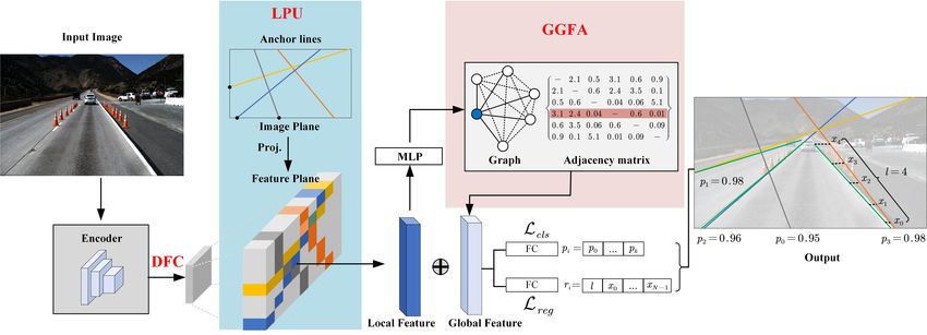
Sensors 2021, 21, 4657                                                                                            2 of 17

                         encoder to generate feature maps from the original image, then use an up-sampling module
                         as the decoder to enlarge the size of feature maps, performing a pixel-wise prediction.
                         However, the lanes are represented as segmented binary features in segmentation methods,
                         which makes it difficult to aggregate the overall information of lanes. Although some
                         works [10,12,14] utilize specially-designedspatial feature aggregation modules to effectively
                         enhance the long-distance perception ability. However, they also increase the computa-
                         tional complexity and make the running speed slower. Moreover, most segmentation-based
                         methods need to use post-processing operations (e.g., clustering) to group the pixel-wise
                         predictions, which is also time-consuming.

                         Figure 1. Examples of complex traffic driving scenarios. Some difficult areas are marked with
                         red arrows.

                               In order to avoid the above-mentioned shortcomings of segmentation-based methods,
                         a great number of works [15–18] began to focus on using different modeling methods
                         to deal with the lane detection problem. Polynomial-based methods [16,18] propose to
                         localize lanes by learnable polynomials. They project the real 3D space into 2D image space
                         and fit a series of point sets to determine the specific coefficients. Row-based classification
                         methods [15,19] detect lanes by row-wise classification based on a grid division of the input
                         image. Anchor-based approaches [17,20] generate a great number of anchor points [20] or
                         anchor lines [17] in images and detect lanes by classifying and regressing them. The above
                         methods consider the strong shape prior of lanes and can extract the local features of
                         lanes more efficiently. Besides, these works discard the heavy decoding network and
                         directly process the high-dimensional features generated by the encoding network, so the
                         real-time ability of them is stronger than segmentation-based methods. However, for fewer
                         calculation and training parameters, most methods above directly use 1 × 1 convolution to
                         compress high-dimensional features to complete downstream tasks (i.e., classification and
                         regression tasks). Because the dimension difference between input features and compressed
                         features is too large, the information loss problem is serious in the feature compression,
                         which affects the upper bound of accuracy.
                               Consider the existing difficulties and the recent development of lane detection, we
                         propose a fast and accurate method to detect lanes, namely FANet, aiming to resolve the
                         three difficulties mentioned in the first paragraph. For the first issue, we utilize a line
                         proposal unit (LPU) to effectively extract the local lane feature with strong discrimination.
                         LPU generates a series of anchor lines over the image space and extracts the thin and long
                         lane features by the locations of anchor lines. For the second problem, we propose a graph-
                         based global feature aggregation module (GGFA) to aggregate global lane features with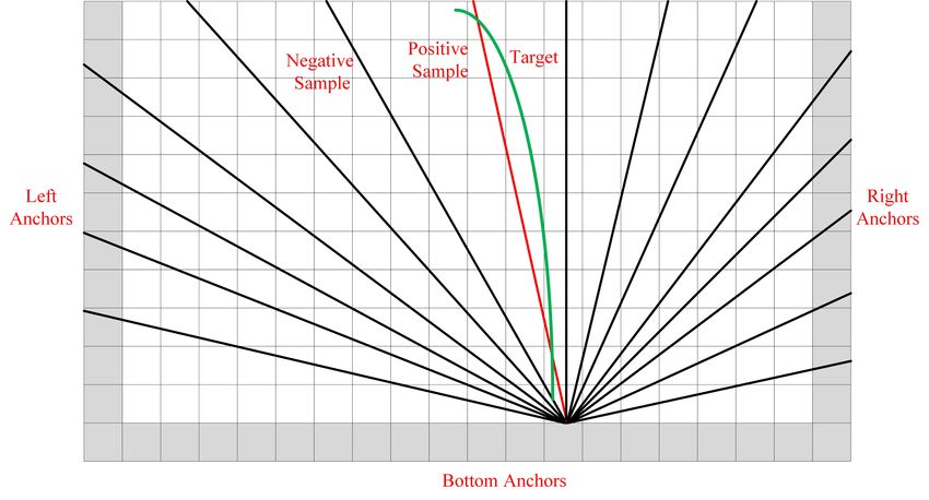
Sensors 2021, 21, 4657                                                                                           3 of 17

                         strong perception. GGFA treats local lane features as nodes of the graph, and adaptively
                         learn the distances between nodes, then utilizes weighted sums to generate global feature.
                         This graph is fully connected, its edges represent the relations between nodes. GGFA can
                         effectively capture visual cues and generate global features with strong perception ability.
                         For the third difficulty, to pursue higher running speed, we also drop the decoder network
                         and compress the high-dimensional feature map as above works. However, unlike they
                         directly use 1 × 1 convolution to compress features, we utilize the idea of disentangled
                         representation learning [21,22] to restain more information in compressed features and
                         name this module as Disentangled Feature Compressor (DFC). Specifically, DFC divides
                         the high-dimensional feature map into three groups and integrates features respectively
                         through low-dimensional 1 × 1 convolution. Then, inspired by batch normalization (BN)
                         operation [23], DFC follows the “normalize and denormalize” steps to learn the statistical
                         information in the spatial dimension, so that the representation of the compressed feature
                         will be richer. Moreover, sufficient experimental results in different scenarios also prove
                         the strong generalization ability of our method.
                              Extensive experiments are conducted on two popular benchmarks, i.e., Tusimple [24]
                         and CULane [10], our proposed FANet achieves higher efficacy and efficiency compared
                         with current state-of-the-art methods. In summary, our main contributions are:
                         •    We propose a fast and accurate lane detection method, which aims to alleviate the
                              main difficulties among lane detection problems. Our method achieves state-of-the-art
                              performance on Tusimple and CULane benchmarks. Besides, the generalization of it
                              is also outstanding in different driving scenarios.
                         •    We propose an efficient and effective global feature aggregator, namely GGFA, which
                              can generate the global lane feature with strong perception. This module is a general
                              module that can apply to other methods whose local features are available.
                         •    We propose a general feature compressor based on disentangled representation learn-
                              ing, namely DFC, which can restrain more information in the compressed feature
                              without speed delay. This module is suitable to feature compression with huge
                              dimensional differences, which can greatly improve the upper bound of accuracy.

                         2. Related Work
                              Lane detection is a basic perceptual task in computer vision and has long been the
                         core of autonomous driving. Due to scene difficulties such as occlusion and illumina-
                         tion changes, as well as realistic requirements such as generalization and real-time, lane
                         detection is still a challenging task. The current deep learning methods can divide into
                         four categories: segmentation-based methods, anchor-based methods, row-based methods,
                         and polynomial-based methods.

                         2.1. Segmentation-Based Methods
                              Segmentation-based methods are the most common manner to detect lanes and have
                         achieved significant success. They locate the positions of lanes by predicting the pixel-level
                         categories of the image. Different from general segmentation tasks, lane detection needs
                         instance-level discrimination, somewhat like an instance segmentation problem. Some
                         methods proposed to utilize multi-class classification to resolve this problem, yet they can
                         only detect a fixed number of lanes. For higher flexibility and accuracy, some methods
                         add a post-clustering strategy to group the lanes. However, this post-process is always
                         time-consuming. Another problem that affects accuracy is that lane detection needs a
                         stronger receptive field than general segmentation tasks due to the long and thin structure
                         of lanes. Bell et al. [25] utilized recurrent neural networks (RNN) to transmit the horizontal
                         and vertical contextual information in the image to improve the spatial structure perception
                         of features. Liang et al. [26] constructed a graph long short-term memory layer (LSTM) to
                         provide a direct connection for spatial long-distance information transmission and enhance
                         the ability of long-distance perception. Pan et al. [10] proposed a specifically designed
                         scheme for long and thin structures and demonstrated its effectiveness in lane detection.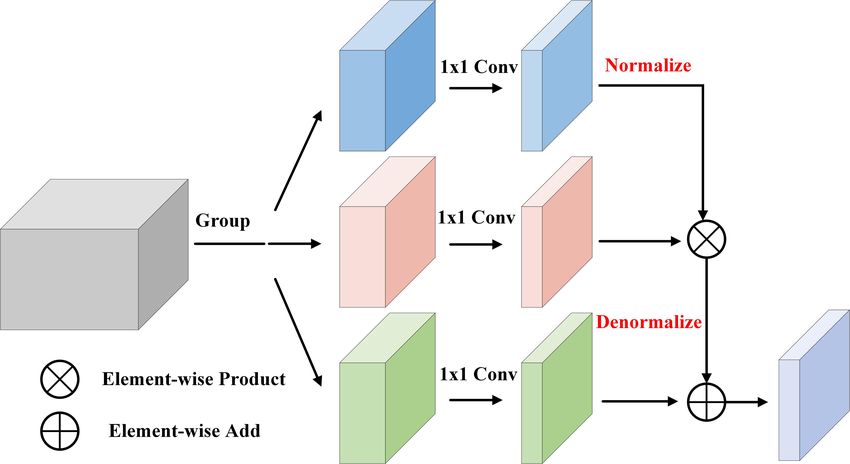
Sensors 2021, 21, 4657 4 of 17
However, the above operations are time-consuming due to the long-distance information
communication. Recently, some studies [19,27] indicated that it is inefficient to describe
the lane as a mask because segmentation-based methods can not emphasize the shape
prior of lanes. To overcome this problem, row-based, polynomial-based, and anchor-based
methods are proposed.
2.2. Row-Based Methods
Row-based methods have a good use of shape prior of lanes and predict locations
of lanes by the classification of each row. They fully utilize the characteristic that lane
lines do not intersect horizontally and add the location constraint of each row to achieve
the continuity and consistency of lanes [19,28]. Besides, some recent row-wise detection
methods [15,19] have achieved advantages in terms of efficiency. But as the widely used
post-clustering module [29] in segmentation-based methods cannot be directly integrated
into the row-wise manner, row-wise methods can only detect fixed lanes by multi-class
classification strategy.
2.3. Polynomial-Based Methods
Polynomial-based methods utilize learnable polynomials on image space to fit the
locations of lanes. PolyLaneNet [16] first proposed to localize lanes by regressing the
lane curve equation. LSTR [18] introduced transformer [30] and Hungarian Algorithm to
achieve a fast end-to-end lane detection method. However, polynomial-based methods
have not surpassed other methods in terms of accuracy. Besides, they usually have a high
bias towards straight lanes in their predictions.
2.4. Anchor-Based Methods
Inspired by the idea of anchor-based detection methods like [31,32], anchor-based
lane detection methods are proposed to generate a great number of anchors. Due to the
slender shape of lane lines, the widely used anchor boxes in object detection cannot be used
directly. Anchor-based lane detection methods usually define a large number of anchor
points [20] or anchor lines [17] to extract local lane feature efficiently, then classify them
into certain categories and regress the relative coordinates.
3. Methods
We first introduce the overall architecture of our proposed FANet in Section 3.1.
Then, the DFC module, a feature compressor that is based on disentangled representation
learning, will be introduced in Section 3.2. Subsequently, Line Proposal Unit (LPU), an
anchor lines generator will be introduced in Section 3.3. The proposed GGFA module,
an effective and efficient global lane feature aggregator, will be introduced in Section 3.4.
Finally, we elaborate on the details of the model training process in Section 3.5.
3.1. Architecture
FANet is a single-stage anchor-based detection model (like YOLOv3 [31] or SSD [32])
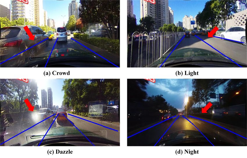
for lane detection. The overview of our method is as shown in Figure 2.
It receives an RGB image I ∈ R HI ×WI ×3 as input, which is taken from the camera
mounted in a vehicle. Then, an encoder (such as ResNet [33]) extracts the features of I,
outputting a high-dimensional feature map FH ∈ R HF ×WF ×C with deep semantic infor-
mation, where HF , WF , and C are the height, the width, and the channel dimension of
FH . For fast running, the DFC module we proposed is then applied into FH and generates
compressed feature FC ∈ R HF ×WF ×Ĉ with a low dimension, where Ĉ is the channel dimen-
sion of FC . After that, LPU generates predefined anchor lines which are throughout the
image and extracts local lane features by their locations from FC . To enhance the percep-
tion of the features, GGFA builds a graph structure and aggregates global lane features
with the input of local lane features. Then, we concatenate the local lane features and the
global features, then predict the lanes by two fully connected layers (FC). The first oneSensors 2021, 21, 4657 5 of 17
is to classify the proposal lanes are background or targets. The second one is to regress
relative coordinates. Since the lane is represented by 2D-points with fixed equally-spaced
y-coordinates, the corresponding x-coordinates and the length of the lane are the targets in
the regression branch.
Figure 2. An overview of our method. An encoder generates high-dimensional feature maps from an input image. DFC is
then applied to reduce the dimension of features. Subsequently, LPU generates a large number of predefined anchor lines.
They are projected onto the feature maps, and the local features can be obtained by pixel-wise extraction. Then, with the
input of the local features, GGFA aggregates the global feature with a strong perception. Finally, the concatenated features
are fed into two layers (one for classification and another for regression) to make the final predictions.
3.2. Disentangled Feature Compressor
Our proposed DFC aims to preserve more information of compressed features, thereby
improving the representation of features. The core of it is to exploit the idea of disentangled
representation learning to reduce the correlation of feature components. Besides, the mod-
ule design is inspired by the classic batch normalization (BN) operation, which follows the
“normalize and denormalize” steps to learn the feature distribution. Next, we will detail
the structure design, the theory, and the computational complexity of our module.
3.2.1. Structure Design
As shown in Figure 3, DFC module receives a high-dimensional feature FH as input,
the size of it is [ H, W, C ]. Then, DFC divides FH into three groups and generates three
low-dimensional feature maps FL1 , FL2 , FL3 through three 1 × 1 convolutions that do not
share weights. The size of the low-dimensional feature map is [ H, W, Ĉ ]. After that,
normalization operation in the spatial dimension is performed onto FL1 , making the features
more compact. Finally, with the input of N ( FL1 ), FL2 , and FL3 , denormalization operation
consisting of element-wise product and element-wise add is then used to learn the spatial
statistical information, thus enhancing the diversity of the compressed feature.Sensors 2021, 21, 4657 6 of 17
Figure 3. The structure design of DFC. Best viewed in colors.
3.2.2. Theory Analysis
As mentioned above, the core of DFC is based on decoupling representation learning,
which can reduce the coupling between features, thereby enhancing feature diversity. Dif-
ferent from common decoupling representation learning tasks [34–36] that branches have
different supervision goals respectively. In our module, the three branches are all super-
vised by the final targets, i.e., classification and regression tasks. Nevertheless, the “divide
and conquer” strategy of decoupling representation learning is exploited in our module.
After deciding the main idea of our module, we make an assumption for the feature
compression problem, i.e., the high-dimensional feature has a great amount of redundant
information, and suitable division does not have much impact on its representation ability.
Therefore, we divide the high-dimensional feature map into three components, each of
which has a different effect on the target.
Inspired by the classic batch normalization algorithm, we apply the “normalize and
denormalize” steps to learn the statistical information in the feature plane. The formulation
of BN is as follows:
Z [l ] − µ
Z̃ [l ] = γ · √ +β (1)
σ2 + e
where γ and β are the learnable parameters to perform the “denormalize” operation. Z [l ]
denotes the l-th sample in a mini-batch. µ and σ are the mean and standard deviation of Z,
e is a small number, preventing the denominator from being zero.
Instead of learning the mini-batch sample distribution in BN, we propose to learn the
spatial feature distribution. The computation is as follows:
1 1
!
2 FL − µs FL
F̃L = FL + FL3 (2)
σs FL1 + e
where µs and σs are the mean and standard deviation of FL1 in the spatial feature dimension.
FL2 and FL3 are analogous to the γ and β in Equation (1), which are also learnable. Therefore,
the three independent components, i.e., FL1 . FL2 , and FL3 all have the different functions
towards the target. FL1 is the component to control the specific value, somewhat like the
“value” component of transformer [30]. FL2 controls the deviation of the main distribution,
and also decides the preservation degree of FL1 . FL3 controls the bias of the distribution.
3.2.3. Computational Complexity
We compare the computational complexity of the 1 × 1 convolution and the DFC
module we designed in this section. The computational complexity of 1 × 1 convolution is
as follows:
Sc = 1 × 1 × H × W × C × Ĉ. (3)Sensors 2021, 21, 4657 7 of 17
While the computational complexity of DFC is written as:
Sd = Sc + O H × W × Ĉ (4)
where the convolution part of two operations is the same, while DFC adds normalization
operation, element-wise product, and element-wise add. The extra computational com-
plexity is far less than Sc . Taking C = 512 and Ĉ = 64 as an example, calculation increment
is only 1%, which can almost be ignorable.
3.3. Line Proposal Unit
The structure of LPU is as shown in Figure 2, which generates a series of anchor lines
and extracts local lane features by their locations. In this way, these local features have a
strong shape prior, i.e., thin and long, thereby having a stronger discrimination ability.
As shown in Figure 4, we define the anchor line as a straight ray. LPU generates lines
from the left, bottom, and right boundaries. A straight ray is set with a certain orientation
θ and each starting point { Xs , Ys } is associated with a group of rays. However, the number
of anchor lines greatly influences the efficiency of the method. Therefore, we exploit the
statistical method to find the most common locations of lanes, thereby reducing the number
of anchor lines. Specifically, we first approximate the curve lanes as straight lines in the
training samples and record the angles and the start coordinates of them. Then, we utilize
K-means clustering algorithm to find the most commonly used clusters, thereby getting
the set of anchor lines. Table 1 shows the results after clustering representative angles.
After getting the set of anchor lines, LPU can extract the feature of each anchor line by
its location, which is composed of many pixel-level feature vectors. To ensure that the
feature dimension of each anchor line is the same, we uniformly sample pixels in the height
dimension of the feature map yi = {0, 1, 2, . . . , HF − 1}. The corresponding x-coordinates
can be obtained by a projection function:
1
xi = (y − Ys /S) + Xs /S (5)
tan θ i
where S is the global stride of the backbone. Then, we can extract the local feature
1 , F2 , . . . , F HF −1 } for each anchor line based on projected coordinates. In cases
Floc = { Floc loc loc
where { xi , yi } is outside the boundaries of FC , Floc i is zero-padded. Finally, the local lane
features Floc ∈ R HF ×Ĉ of anchor lines with the same dimension can be obtained.
Figure 4. The illustration of anchor line generation process. The green line is the target lane. The red
line is the anchor line closest to the target, which is treated as the positive sample. The black lines
are negative samples. The gray grids are the starting coordinates for generating the anchor line,
including left anchors, bottom anchors, and right anchors.Sensors 2021, 21, 4657 8 of 17
Table 1. The angel setting of anchor lines.
Boundary N The Set of Angles
left 6 72◦ 60◦ 49◦ 39◦ 30◦ 22◦
right 6 108◦ 120◦ 131◦ 141◦ 150◦ 158◦
bottom 15 165 150 141 131◦ 120◦ 108◦ 100◦ 90◦ 80◦ 72◦ 60◦ 49◦ 39◦ 30◦ 15◦
◦ ◦ ◦
3.4. Graph-Based Global Feature Aggregator
Lane detection requires a strong perception to locate the positions of lanes, but the
local features cannot effectively perceive the global structure of the image, thus we propose
GGFA to extract global lane features based on graph structure.
The structure of GGFA is as shown in Figure 5. It receives the local lane features
Floc ∈ R HF ×Ĉ as input and outputs the global lane features Fglb ∈ R HF ×Ĉ , which have the
same dimension as Floc . Specifically, with the input of Floc , Multi-Layer Perceptron (MLP)
2
generates a distance vector with N 2− N dimensions. Then, the distance vector is filled in the
upper half part of an all-zero matrix. Flipping operation is applied to this matrix, making it
perform as an axisymmetric matrix. In this way, the graph constructed by local features is
a fully connected undirected graph. The distance between two nodes is the same for each
one. After that, the weight matrix can be got as follows:
e Di,j
Wi,j = 1 − D
(6)
∑ j e i,j
| {z }
Softmax
where Di,j is the distance between i-th and j-th nodes. Softmax operation transforms the
distances to a soft value, then 1 reduces this soft value, which represents the similarity of
two nodes. The distance between the two nodes is closer, the similarity weight will be
bigger. After performing matrix transpose and element-wise product operation, the global
feature Fglb can be obtained finally.
Figure 5. The structure of GGFA. For better visualization, we add the batch dimension B to the local
feature, performing in a three-dimensional manner. N represents the number of pixels in each anchor
line, which is equal as HF . D is the feature dimension, which is equal as Ĉ.Sensors 2021, 21, 4657 9 of 17
This module learns the relationship between the local features by constructing the
graph structure. Because the anchor lines are all over the whole image, the learned global
features also fully consider the spatial relationship and visual cues. Therefore, the local features
with long-distance can also be effectively communicated, thus enhancing the perception of
features. At the same time, using adaptive weighted summation, the importance of each local
feature can also be distinguished, making the learned global features informative.
3.5. Module Training
Similar to object detection, anchor-based lane detection methods also need to define
a function to measure the distance between two lanes. For two lanes with common
Npts
valid indices (i.e., equal-distance y-coordinates), the x-coordinates are Xa = { xia }i=1 and
Npts
Xb = { xib }i=1 , respectively, where Npts is the number of common points. The lane distance
metric proposed in [17] is adopted to compute the distance between two lanes:
0
(
1
e 0 − s 0 +1 · ∑ie=s0 xia − xib , e0 ≥ s0
D ( X a , Xb ) = (7)
+∞, else
where s a and sb are the start valid indices of two lanes, ea and eb are the end valid in-
dices of two lanes, and s0 = max (s a , sb ) and e0 = min(ea , eb ) define the range of those
common indices.
Based on the distance metric in Equation (7), the process of training sample assignment
can be defined. We compute the distance between anchor lines and targets, the anchor
lines with a distance lower than a threshold τp are considered as positive samples, while
those with a distance larger than a threshold τn are considered as negative samples.
The final loss function consists of two components, i.e., classification loss and regres-
sion loss, which are implemented by Focal loss [37] and L1 loss, respectively. The total loss
can be defined as:
N −1
L {pi , ri }i=p&n
0 =λ ∑ Lcls (pi , pi∗ )
i
(8)
+ ∑ Lreg (ri , ri∗ )
i
where Np&n is the number of positive and negative samples, λ is used to balance the loss
terms, pi , ri are the classification and regression predictions of the i-th anchor line, and pi∗ ,
ri∗ are the corresponding classification and regression targets. pi∗ consists of “0” and “1”,
i.e., background and lanes. ri∗ is composed with the length l and the x-coordinates.
4. Experiments
In this section, we first introduce the datasets of our experiments, i.e., Tusimple [24]
and CULane [10] benchmarks in Section 4.1, then present the implementation details of our
methods in Section 4.2. After that, we compare the performance of our proposed FANet
with other SOTA methods in Section 4.3 and conduct sufficient ablation studies to prove
the effectiveness of our proposed modules in Section 4.4.
4.1. Dataset
Tusimple [24] and CULane [10] are the most popular benchmarks in lane detection.
The TuSimple dataset is collected with stable lighting conditions in highways. The CULane
dataset consists of nine different scenarios, including normal, crowd, dazzle, shadow, no
line, arrow, curve, cross, and night in urban areas. More details about these datasets can be
seen in Table 2.Sensors 2021, 21, 4657 10 of 17
Table 2. Dataset description.
Dataset #Frame Train Validation Test Resolution #Lane #Scenarios Environment
TuSimple [24] 6408 3268 358 2782 1280 × 720 ≤5 1 highway
CULane [10] 133,235 88,880 9675 34,680 1640 × 590 ≤4 9 urban and highway
4.1.1. TuSimple
TuSimple is a lane detection dataset for highway scenes, which is used for the primary
evaluation of lane detection methods. This dataset contains 3626 training images and
2782 test images. The image size in TuSimple is 1280 × 720, and each image contains up
to 5 lanes.
On TuSimple, the main evaluation metric is accuracy, which is computed as:
∑clip Cclip
accuracy = (9)
∑clip Sclip
where Cclip is the number of lane points that are predicted correctly and Sclip is the total
number of evaluation points in each clip. For each evaluation point, if the predicted point
and the target point are within 20-pixel values, the prediction is considered to be correct,
otherwise wrong. Moreover, we also calculate the false-positive rate (FP), the false-negative
rate (FN), and the F1 score on predictions.
4.1.2. CULane
CULane is a large lane detection dataset containing multiple scenarios. CULane has
98,555 training images and 34,680 test images. The image size is 1640 × 590, and each
image contains up to 4 lanes.
The evaluation metric of CULane benchmark is F1 score, which can be defined as:
2 × Precision × Recall
F1 = (10)
Precision + Recall
where Precision = TPTP TP
+ FP and Recall = TP+ FN . Different from TuSimple, each lane is
considered as a line with a width of 30 pixels. Intersection-over-union (IoU) is calculated
between predictions and targets. Those predictions with IoUs larger than a threshold (e.g.,
0.5) are considered as correct.
4.2. Implementation Details
For all datasets, the input images are resized to 360 × 640 by bilinear interpolation
during training and testing. Then, we utilize a random affine transformation (with trans-
lation, rotation, and scaling) along with random horizontal flips for data augmentaion.
Adam [38] is adopted as the optimizer for training, the epoch is 100 in Tusimple dataset
and 15 in CULane dataset. Learning rate is set to 0.003 with the CosineAnnealingLR learning
rate schedule. To ensure the consistency of the experimental environment, all experimental
results and speed measurements are performed on a single RTX 2080 Ti GPU. The number
of anchor lines is set to 1000, the number of evaluation points (Npts ) is 72, the threshold for
positive samples (τp ) is set to 15, and the threshold for negative samples (τn ) is set to 20.
To ensure the invisibility of the test dataset during the training process, we divide a
small part of the two datasets as validation datasets for saving the optimal model. 358 and
9675 images were selected in TuSimple and CULane datasets, respectively.
4.3. Comparisons with State-of-the-Art Methods
In this section, we compare our FANet with other state-of-the-art methods on TuSimple
and CULane benchmarks. In addition to the F1 score and accuracy, we also evaluate the
running speed (FPS) and calculation amount (MACs) for a fair comparison.Sensors 2021, 21, 4657 11 of 17
For TuSimple benchmark, the results of FANet along with other state-of-the-art meth-
ods are shown in Table 3. Our proposed FANet performs the best in F1 score and also
achieves good performance in other metrics. It is clear that the accuracy in TuSimple is
relatively saturated, and the accuracy improvement in state-of-the-art methods is also small.
Nevertheless, our proposed FANet also performs high accuracy with high efficacy simulta-
neously. FANet is 33 times faster than SCNN [10], almost 8 times faster than Line-CNN [17],
about 3 times faster than ENet-SAD [12], and 2 times faster than PolyLaneNet [16]. Com-
pared with the UFLD [19], although it runs faster than ours, the false positive rate of UFLD
is too high, reaching 19.05%, making it difficult to be applied to actual scenarios.
Table 3. State-of-the-art comparisons on TuSimple. For fair comparison, frames per second (FPS)
was measured on the same machine used by our method. The best and second-best results across
methods are shown in boldface and underlined, respectively. These blank values indicate that the
results are not published in their papers, and their codes and models are not available either.
Method F1 (%) Acc (%) FP (%) FN (%) FPS MACs (G)
FastDraw [28] 94.59 94.90 6.10 4.70
Line-CNN [17] 96.79 96.87 4.42 1.97 30.0
PointLaneNet [20] 95.07 96.34 4.67 5.18 71.0
E2E-LMD [15] 96.40 96.04 3.11 4.09
SCNN [10] 95.97 96.53 6.17 1.80 7.5
ENet-SAD [12] 95.92 96.64 6.02 2.05 75.0
UFLD [19] 87.87 95.82 19.05 3.92 425.0
PolyLaneNet [16] 90.62 93.36 9.42 9.33 115.0 1.7
FANet (Ours) 96.81 95.71 3.66 2.86 248.0 9.3
For CULane benchmark, the results of FANet along with other state-of-the-art methods
are as shown in Table 4. Our FANet achieves state-of-the-art performance while with high
running speed. In crowded, dazzle, no line, cross, and night scenarios, FANet outperforms
the other methods. Compared with SIM-CycleGAN [39], although it is specifically designed
for different scenarios, FANet is also close to it in many metrics, or even better. Compared
with the knowledge distillation method IntRA-KD [14] and the network search method
CurveLanes-NAS [40], FANet has a higher F1 score of 3.09% and 4.09% F1 respectively.
Compared with UFLD, although it is faster than ours, FANet outperforms it with a 7.09%
F1 score.
Table 4. State-of-the-art comparisons on CULane. For fair comparison, frames per second (FPS) was measured on the same
machine used by our method. Because the images in “Cross” scene have no lanes, only false positives are shown. The best
and second-best results across methods are shown in boldface and underlined, respectively. These blank values indicate
that the results are not published in their papers, and their codes and models are not available either.
Method Total Normal Crowded Dazzle Shadow No line Arrow Curve Cross Night FPS MACs (G)
E2E-LMD [15] 70.80 90.00 69.70 60.20 62.50 43.20 83.20 70.30 2296 63.30
SCNN [10] 71.60 90.60 69.70 58.50 66.90 43.40 84.10 64.40 1990 66.10 7.5
ENet-SAD [12] 70.80 90.10 68.80 60.20 65.90 41.60 84.00 65.70 1998 66.00 75.0
IntRA-KD [14] 72.40 100.0
SIM-CycleGAN [39] 73.90 91.80 71.80 66.40 76.20 46.10 87.80 67.10 2346 69.40
CurveLanes [40] 71.40 88.30 68.60 63.20 68.00 47.90 82.50 66.00 2817 66.20 9.0
UFLD [19] 68.40 87.70 66.00 58.40 62.80 40.20 81.00 57.90 1743 62.10 425.0
FANet (Ours) 75.49 91.30 73.45 67.22 70.00 48.73 86.36 64.18 1007 69.45 248.0 9.3
The visualization results of FANet on TuSimple and CULane are also shown in
Figure 6. Although the anchor lines are all straight in FANet, it does not affect the fit-
ting of curved lane lines, as shown in the second row of Figure 6. Besides, FANet also hasSensors 2021, 21, 4657 12 of 17
a strong generalization in various scenarios, such as dazzle, crowded, and night scenes,
as shown in the fourth row of Figure 6.
Figure 6. Visualization results on TuSimple (top two rows) and CULane (middle two rows). Blue lines are ground-truth and
green lines are predictions.
4.4. Ablation Study
4.4.1. The Number Setting of Anchor Lines
Efficiency is crucial for a lane detection model. In some cases, it even needs to trade
some accuracy to achieve the application’s requirement. In this section, we compare the
performance of different numbers of anchor lines settings. In addition to the F1 score,
we also compared the running speed (FPS), calculation complexity (MACs), and training
time (TT).
As shown in Table 5, until the number of anchor lines is equal to 1000, as the number
increases, the F1 score also increases. However, if there are too many anchor lines, i.e., 1250,
the F1 score will drop slightly. During the inference phase, the predicted proposals are
filtered by non-maximum suppression (NMS), and its running time depends directly on
the number of proposals, therefore the number of anchor lines directly affects the running
speed of the method.Sensors 2021, 21, 4657 13 of 17
Table 5. The efficiency trade-offs of different anchor line numbers on CULane using the ResNet-18
backbone.“TT” represents the training time in hours.
N F1 (%) FPS MACs (G) TT (h)
250 67.32 281 8.7 4.6
500 73.56 274 8.8 5.3
750 74.10 263 9.1 6.8
1000 75.49 248 9.3 10.2
1250 75.42 231 9.7 10.6
4.4.2. The Effect of Graph-Based Global Feature Aggregator
As shown in Table 6, under the same backbone network, i.e., ResNet-18, the F1 value
is 74.02% when GGFA is not added, and the F1 value is increased to 75.05% after adding
GGFA, an increase of 1.03%. The performance improvement shows that our proposed
GGFA can effectively capture global information by long-distance weight learning. At the
same time, the performance gap also proves the importance of global features with strong
perception for lane detection.
Table 6. The effectiveness of GGFA.
Method Backbone F1 (%)
w/o GGFA ResNet-18 74.02
w/ GGFA ResNet-18 75.05 (+1.03)
GGFA measures the distance between anchor lines by MLP and generates similarity
through softmax operation. To better observe the relationship between the various anchor
line features, we draw the three most similar anchor lines of the predicted lanes, as shown
in Figure 7. It is clear that the anchor lines with big similarities are always close to the
predicted lanes. Besides, these anchor lines always focus on some visual cues, e.g., light
changes and occlusion, which makes the method can capture some important information.
Figure 7. Cont.Sensors 2021, 21, 4657 14 of 17
Figure 7. Intermediate visual results of GGFA. The three most similar anchor lines are represented
by dashed lines. Different lanes are drawn by different colors.
4.4.3. Performance Comparison under Different Groupings in DFC
As mentioned in Section 3.2, DFC divides the high-dimensional feature into three
groups. In this part, we further research the effect of different grouping methods, i.e., block,
interval, and random methods. The block method directly divides the high-dimensional
features into three groups according to the original arrangement order; the interval method
internally takes out the high-dimensional features according to the number of channels,
and puts them in three groups; the random method divides the high-dimensional features
into three groups after shuffling in the channel dimension.
As shown in Table 7, It is clear that the interval method achieves the best performance,
and the random method achieves the second performance, yet the performance of the
block method has a large gap. For the feature of each group, the first two methods cover
the full range of original channels while the block method only takes the information of
1/3 area. The block method breaks the structure of the original feature, so resulting in
an accuracy gap. It also proves the assumption we proposed, i.e., the high-dimensional
feature has a great amount of redundant information, the suitable division does not affect
its representation ability.
Table 7. The influence of different grouping methods on DFC. The best result is marked in bold.
Grouping Method Backbone F1 (%)
Block ResNet-18 75.17
Interval ResNet-18 75.49
Random ResNet-18 75.35
4.4.4. The Effect of Different Channel Dimensions in DFC
To verify the effect of our proposed DFC module, we apply it to high-dimensional
feature compression with different dimensions. ResNet-18 and ResNet-50 are used to
generate 512 and 2048 dimensions of features, respectively. In ResNet-18, high-dimensional
features are compressed from 512 to 64 dimensions while 2048 to 64 in ResNet-50. In terms
of task difficulty, it is undoubtedly more difficult to reduce feature dimensions from 2048
to 64.
As shown in Table 8, compared with 1 × 1 convolution, our proposed DFC achieves
0.44% F1 score improvement in ResNet-18, and 0.78% F1 score improvement in ResNet-50.
With the same 64-dimensional compressed features, the accuracy is improved significantly
after applying our proposed DFC module. It proves that DFC can indeed preserve more
information compared with 1 × 1 convolution. Besides, the performance improvement of
DFC is more obvious when the feature dimension is higher. It shows that DFC performs bet-
ter when the dimensional difference is great. At the same time, the consistent improvement
in different dimensions also proves the effectiveness and strong generalization of DFC.Sensors 2021, 21, 4657 15 of 17
Table 8. The effect of different channel dimensions in DFC. 1 × 1 Conv means 1 × 1 convolution.
Method Dimension Backbone F1 (%)
1 × 1 Conv 512 ResNet-18 75.05
DFC 512 ResNet-18 75.49 (+0.44)
1 × 1 Conv 2048 ResNet-50 75.46
DFC 2048 ResNet-18 76.24 (+0.78)
5. Discussion
According to the results in Table 4, our proposed FANet is not ideal to detect curve
lanes. Compared with other scenarios, the results of the curve scene are unsatisfactory.
Therefore, we discuss the reason for this phenomenon.
We first make a visualization towards the curve scene in CULane. As shown in
Figure 8, it is clear that the predictions are straight. The predictions only find the locations
of target lanes and do not fit the curvature of lanes. However, the predictions of TuSimple
are indeed curved as shown in Figure 6. Therefore, this is not the problem of the model or
code implementation.
Figure 8. Curve lanes predictions on CULane.
We further discuss CULane dataset itself. As shown in Table 9, we count the number
of images in various scenarios in CULane. We found that curve lanes are rare in CULane,
which are only 1.2% of training images. It means that almost all the lanes in CULane are
straight, result in significant bias. It can also explain why the predictions of our model are
all straight in CULane.
Table 9. The image number of different scenarios in CULane.
Normal Crowded Dazzle Shadow No Line Arrow Curve Cross Night
9621 8113 486 930 4067 890 422 3122 7029
However, after confirmation, we found that the prediction results in Figure 8 are
all regarded as correct because of the high degree of coincidence. Therefore, it can not
explain the accuracy gap compared with other methods in the curve scene. Then, we train
the model many times and found the experimental results in the curve scene fluctuate
greatly. As shown in Table 10, the accuracy gap between the best and the worst is huge,
i,e., 2.36 % F1 score. It seems that the few training samples of the curve scene make the
accuracy unstable.
Table 10. The results of multiple experiments on the curve scene in CULane.
1-th 2-th 3-th 4-th 5-th
64.18 63.74 65.53 66.10 64.62Sensors 2021, 21, 4657 16 of 17
6. Conclusions
In this paper, we proposed a fast and accurate lane detection method, namely FANet.
FANet alleviates three main difficulties of lane detection: (1) how to efficiently extract local
lane features with strong discrimination ability; (2) how to effectively capture long-distance
visual cues; (3) how to achieve strong real-time ability and generation ability. For the first
difficulty, we utilize Line Proposal Unit (LPU) to generate anchor lines over the image
with strong shape prior, and efficiently extract local features by their locations. For the
second difficulty, we propose a Graph-based Global Feature Aggregator (GGFA), which
treats local features as nodes and learns global lane features with strong perception by
establishing graph structure. For the third difficulty, our goal is to improve the accuracy
of the model without affecting the running speed. Therefore, we propose a Disentangled
Feature Compressor (DFC), which is a general and well-designed module for feature
compression with a large dimension gap. DFC greatly improves the upper bound of
accuracy while without speed delay. We also evaluate the generation of our method in
various scenarios, the consistent outstanding performance proves the strong generation
ability of FANet.
Author Contributions: Methodology and writing—original draft, Y.H.; supervision and project ad-
ministration, W.C.; data curation and formal analysis, C.L.; writing—review and editing, X.L.; project
administration, L.H. All authors have read and agreed to the published version of the manuscript.
Funding: This work was supported by the National Key Research and Development Program of
China (No. 2018YFB0204301), NSFC (No. 61872374).
Institutional Review Board Statement: Not applicable.
Informed Consent Statement: Not applicable.
Data Availability Statement: Not applicable.
Conflicts of Interest: The authors declare no conflict of interest.
References
1. Hillel, A.B.; Lerner, R.; Levi, D.; Raz, G. Recent progress in road and lane detection: A survey. Mach. Vis. Appl. 2014, 25, 727–745.
[CrossRef]
2. Liu, G.; Wörgötter, F.; Markelić, I. Combining statistical hough transform and particle filter for robust lane detection and tracking.
In Proceedings of the 2010 IEEE Intelligent Vehicles Symposium, La Jolla, CA, USA, 21–24 June 2010; pp. 993–997.
3. Zhou, S.; Jiang, Y.; Xi, J.; Gong, J.; Xiong, G.; Chen, H. A novel lane detection based on geometrical model and gabor filter. In
Proceedings of the 2010 IEEE Intelligent Vehicles Symposium, La Jolla, CA, USA, 21–24 June 2010; pp. 59–64.
4. Hur, J.; Kang, S.N.; Seo, S.W. Multi-lane detection in urban driving environments using conditional random fields. In Proceedings
of the 2013 IEEE Intelligent Vehicles Symposium (IV), Gold Coast, QLD, Australia, 23–26 June 2013; pp. 1297–1302.
5. Kim, Z. Robust lane detection and tracking in challenging scenarios. IEEE Trans. Intell. Transp. Syst. 2008, 9, 16–26. [CrossRef]
6. Jiang, R.; Klette, R.; Vaudrey, T.; Wang, S. New lane model and distance transform for lane detection and tracking. In Proceedings
of the International Conference on Computer Analysis of Images and Patterns, Münster, Germany, 2–4 September 2009; Springer:
Berlin/Heidelberg, Germany, 2009; pp. 1044–1052.
7. Daigavane, P.M.; Bajaj, P.R. Road lane detection with improved canny edges using ant colony optimization. In Proceedings of
the 2010 3rd International Conference on Emerging Trends in Engineering and Technology, Goa, India, 19–21 November 2010;
pp. 76–80.
8. Mandalia, H.M.; Salvucci, M.D.D. Using support vector machines for lane-change detection. In Proceedings of the Human Factors
and Ergonomics Society Annual Meeting; SAGE Publications: Los Angeles, CA, USA, 2005; Volume 49, pp. 1965–1969.
9. Neven, D.; De Brabandere, B.; Georgoulis, S.; Proesmans, M.; Van Gool, L. Towards end-to-end lane detection: An instance
segmentation approach. In Proceedings of the 2018 IEEE Intelligent Vehicles Symposium (IV), Changshu, China, 26–30 June 2018;
pp. 286–291.
10. Pan, X.; Shi, J.; Luo, P.; Wang, X.; Tang, X. Spatial as deep: Spatial cnn for traffic scene understanding. In Proceedings of the
AAAI Conference on Artificial Intelligence, New Orleans, LA, USA, 2–7 February 2018; Volume 32.
11. Ko, Y.; Jun, J.; Ko, D.; Jeon, M. Key points estimation and point instance segmentation approach for lane detection. arXiv 2020,
arXiv:2002.06604.
12. Hou, Y.; Ma, Z.; Liu, C.; Loy, C.C. Learning lightweight lane detection cnns by self attention distillation. In Proceedings of the
IEEE/CVF International Conference on Computer Vision, Seoul, Korea, 27–28 October 2019; pp. 1013–1021.Sensors 2021, 21, 4657 17 of 17
13. Lee, S.; Kim, J.; Shin Yoon, J.; Shin, S.; Bailo, O.; Kim, N.; Lee, T.H.; Seok Hong, H.; Han, S.H.; So Kweon, I. Vpgnet: Vanishing
point guided network for lane and road marking detection and recognition. In Proceedings of the IEEE International Conference
on Computer Vision, Venice, Italy, 22–29 October 2017; pp. 1947–1955.
14. Hou, Y.; Ma, Z.; Liu, C.; Hui, T.W.; Loy, C.C. Inter-region affinity distillation for road marking segmentation. In Proceedings of
the IEEE/CVF Conference on Computer Vision and Pattern Recognition, Seattle, WA, USA, 14–19 June 2020; pp. 12486–12495.
15. Yoo, S.; Lee, H.S.; Myeong, H.; Yun, S.; Park, H.; Cho, J.; Kim, D.H. End-to-end lane marker detection via row-wise classification.
In Proceedings of the IEEE/CVF Conference on Computer Vision and Pattern Recognition Workshops, Seattle, WA, USA, 14–19
June 2020; pp. 1006–1007.
16. Tabelini, L.; Berriel, R.; Paixao, T.M.; Badue, C.; De Souza, A.F.; Oliveira-Santos, T. PolyLaneNet: Lane estimation via deep
polynomial regression. arXiv 2020, arXiv:2004.10924.
17. Li, X.; Li, J.; Hu, X.; Yang, J. Line-CNN: End-to-End Traffic line detection with line proposal unit. IEEE Trans. Intell. Transp. Syst.
2019, 21, 248–258. [CrossRef]
18. Liu, R.; Yuan, Z.; Liu, T.; Xiong, Z. End-to-end lane shape prediction with transformers. In Proceedings of the IEEE/CVF Winter
Conference on Applications of Computer Vision, Waikoloa, HI, USA, 5–9 January 2021; pp. 3694–3702.
19. Qin, Z.; Wang, H.; Li, X. Ultra fast structure-aware deep lane detection. arXiv 2020, arXiv:2004.11757.
20. Chen, Z.; Liu, Q.; Lian, C. PointLaneNet: Efficient end-to-end CNNs for Accurate Real-Time Lane Detection. In Proceedings of
the 2019 IEEE Intelligent Vehicles Symposium (IV), Paris, France, 9–12 June 2019; pp. 2563–2568.
21. Liu, W.; Liu, Z.; Yu, Z.; Dai, B.; Lin, R.; Wang, Y.; Rehg, J.M.; Song, L. Decoupled networks. In Proceedings of the IEEE Conference
on Computer Vision and Pattern Recognition, Salt Lake City, UT, USA, 18–23 June 2018; pp. 2771–2779.
22. Ma, J.; Cui, P.; Kuang, K.; Wang, X.; Zhu, W. Disentangled graph convolutional networks. In Proceedings of the International
Conference on Machine Learning, Long Beach, CA, USA, 10–15 June 2019; pp. 4212–4221.
23. Ioffe, S.; Szegedy, C. Batch normalization: Accelerating deep network training by reducing internal covariate shift. In Proceedings
of the International Conference on Machine Learning, Lille, France, 6–11 July 2015; pp. 448–456.
24. TuSimple. Tusimple Benchmark. 2017. Available online: https://github.com/TuSimple/tusimple-benchmark (accessed on 30 July 2017).
25. Bell, S.; Zitnick, C.L.; Bala, K.; Girshick, R. Inside-outside net: Detecting objects in context with skip pooling and recurrent neural
networks. In Proceedings of the IEEE Conference on Computer Vision and Pattern Recognition, Las Vegas, NV, USA, 27–30 June
2016; pp. 2874–2883.
26. Liang, X.; Shen, X.; Feng, J.; Lin, L.; Yan, S. Semantic object parsing with graph lstm. In Proceedings of the European Conference
on Computer Vision, Amsterdam, The Netherlands, 11–14 October 2016; pp. 125–143.
27. Chougule, S.; Koznek, N.; Ismail, A.; Adam, G.; Narayan, V.; Schulze, M. Reliable multilane detection and classification by
utilizing CNN as a regression network. In Proceedings of the European Conference on Computer Vision (ECCV) Workshops,
Munich, Germany, 4–18 September 2018.
28. Philion, J. FastDraw: Addressing the long tail of lane detection by adapting a sequential prediction network. In Proceedings of the
IEEE/CVF Conference on Computer Vision and Pattern Recognition, Long Beach, CA, USA, 15–20 June 2019; pp. 11582–11591.
29. De Brabandere, B.; Neven, D.; Van Gool, L. Semantic instance segmentation with a discriminative loss function. arXiv 2017,
arXiv:1708.02551.
30. Vaswani, A.; Shazeer, N.; Parmar, N.; Uszkoreit, J.; Jones, L.; Gomez, A.N.; Kaiser, L.; Polosukhin, I. Attention is all you need.
arXiv 2017, arXiv:1706.03762.
31. Redmon, J.; Farhadi, A. Yolov3: An incremental improvement. arXiv 2018, arXiv:1804.02767.
32. Liu, W.; Anguelov, D.; Erhan, D.; Szegedy, C.; Reed, S.; Fu, C.Y.; Berg, A.C. Ssd: Single shot multibox detector. In Proceedings of
the European Conference on Computer Vision, Amsterdam, The Netherlands, 8–16 October 2016; Springer: Cham, Switzerland,
2016; pp. 21–37.
33. He, K.; Zhang, X.; Ren, S.; Sun, J. Deep residual learning for image recognition. In Proceedings of the IEEE Conference on
Computer Vision and Pattern Recognition, Las Vegas, NV, USA, 27–30 June 2016; pp. 770–778.
34. Song, G.; Liu, Y.; Wang, X. Revisiting the sibling head in object detector. In Proceedings of the IEEE/CVF Conference on
Computer Vision and Pattern Recognition, Seattle, WA, USA, 14–19 June 2020; pp. 11563–11572.
35. Wu, Y.; Chen, Y.; Yuan, L.; Liu, Z.; Wang, L.; Li, H.; Fu, Y. Rethinking classification and localization for object detection. In
Proceedings of the IEEE/CVF Conference on Computer Vision and Pattern Recognition, Seattle, WA, USA, 14–19 June 2020;
pp. 10186–10195.
36. Jiang, B.; Luo, R.; Mao, J.; Xiao, T.; Jiang, Y. Acquisition of localization confidence for accurate object detection. In Proceedings of
the European Conference on Computer Vision (ECCV), Munich, Germany, 4–18 September 2018; pp. 784–799.
37. Lin, T.Y.; Goyal, P.; Girshick, R.; He, K.; Dollár, P. Focal loss for dense object detection. In Proceedings of the IEEE International
Conference on Computer Vision, Venice, Italy, 22–29 October 2017; pp. 2980–2988.
38. Kingma, D.P.; Ba, J. Adam: A method for stochastic optimization. arXiv 2014, arXiv:1412.6980.
39. Liu, T.; Chen, Z.; Yang, Y.; Wu, Z.; Li, H. Lane detection in low-light conditions using an efficient data enhancement: Light
conditions style transfer. In Proceedings of the 2020 IEEE Intelligent Vehicles Symposium (IV), Las Vegas, NV, USA, 19 October–13
November 2020; pp. 1394–1399.
40. Li, Z. CurveLane-NAS: Unifying Lane-Sensitive Architecture Search and Adaptive Point Blending. In Proceedings of the
European Conference on Computer Vision, Glasgow, UK, 23–28 August 2016; Springer: Cham, Switzerland, 2020.You can also read