Diffuse Skylight as a Surrogate for Shadow Detection in High-Resolution Imagery Acquired Under Clear Sky Conditions - MDPI
←
→
Page content transcription
If your browser does not render page correctly, please read the page content below
remote sensing
Article
Diffuse Skylight as a Surrogate for Shadow Detection
in High-Resolution Imagery Acquired Under Clear
Sky Conditions
Mark Cameron * and Lalit Kumar              ID

 Ecosystem Management, School of Environmental and Rural Science, University of New England, Armidale,
 NSW 2351, Australia; lkumar@une.edu.au
 * Correspondence: mcamer29@myune.edu.au; Tel.: +61-2-6654-8287

 Received: 1 July 2018; Accepted: 25 July 2018; Published: 27 July 2018

 Abstract: An alternative technique for shadow detection and abundance is presented for high
 spatial resolution imagery acquired under clear sky conditions from airborne/spaceborne sensors.
 The method, termed Scattering Index (SI), uses Rayleigh scattering principles to create a diffuse
 skylight vector as a shadow reference. From linear algebra, the proportion of diffuse skylight in
 each image pixel provides a per pixel measure of shadow extent and abundance. We performed
 a comparative evaluation against two other methods, first valley detection thresholding (extent)
 and physics-based unmixing (extent and abundance). Overall accuracy and F-score measures are
 used to evaluate shadow extent on both Worldview-3 and ADS40 images captured over a common
 scene. Image subsets are selected to capture objects well documented as shadow detection anomalies,
 e.g., dark water bodies. Results showed improved accuracies and F-scores for shadow extent and
 qualitative evaluation of abundance show the method is invariant to scene and sensor characteristics.
 SI avoids shadow misclassifications by avoiding the use of pixel intensity and the associated
 limitations of binary thresholding. The method negates the need for complex sun-object-sensor
 corrections, it is simple to apply, and it is invariant to the exponential increase in scene complexity
 associated with higher-resolution imagery.

 Keywords: imagery; shadow; shadow detection; illumination; vector; diffuse skylight;
 high resolution

1. Introduction
      The effects of shadow and illumination are intrinsic to optical remote sensing imagery of the
Earth’s surface. Shadow effects are unique in imagery because their presence is caused by the
obstruction of light from a source of illumination, not by the properties of a surface material [1].
In imagery, shadow presents as a change in radiance value that adds inaccuracies to already complex
Earth scenes captured in high resolution. Accurate detection and quantification of shadow is critical
for its removal and results in improvements for image classification procedures [2].
      To understand the physics of shadows is an important prerequisite for any detection technique.
The physics of shadows are detailed in Funka-Lea and Bajcsy [1], where two shadow types are
described: cast and self-cast. Both types are caused by the obstruction of light by an object, but cast
shadow does not present on the obstructing object whereas self-cast shadow does. Cast shadow has
two characteristics that are defined as umbra and penumbra [1] and shown in Figure 1.

Remote Sens. 2018, 10, 1185; doi:10.3390/rs10081185                       www.mdpi.com/journal/remotesensing
Remote Sens. 2018, 10, 1185 2 of 21
Remote Sens. 2018, 10, x FOR PEER REVIEW 2 of 20
Remote Sens. 2018, 10, x FOR PEER REVIEW 2 of 20
Figure 1. Shadow
Figure1.1. definitions
Shadowdefinitions adopted from
definitionsadopted
adopted from Arévalo,
Arévalo, et
et al.
al. [3].
[3].
Figure Shadow from Arévalo, et al. [3].
Umbra is that part of cast shadow where the light source is completely obstructed compared to
Umbra
Umbraisisthat
thatpart
partof ofcast
cast shadow
shadowwherewhere the
the light
light source
source isis completely
completely obstructed
obstructedcompared
comparedtoto
penumbra where the light source is partially obstructed [1,4]. Dare [4] estimated penumbra location
penumbra
penumbra where
where the
the light
light source
source is is partially
partially obstructed
obstructed [1,4].
[1,4]. Dare
Dare [4]
[4] estimated
estimated penumbra
penumbra location
location
and extent using Equation (1) for an urban building on a flat horizontal ground, shown in Figure 2.
and
and extent
extent using
using Equation
Equation (1)(1) for
for an
an urban
urban building
building onon aa flat
flat horizontal
horizontal ground, shown in Figure 2.
1 1
=
11 − 11
!
(1)
w== H− − − +ε (1)(1)
Tan e − − 2ε2 Tan e + + 22
2 2
where w is penumbra width, building height , sun elevation e and angular width of sun .
where
where w
wisispenumbra
penumbrawidth,
width,building height H,, sun elevation e and angular width of sun ε..
building height
Figure 2. Penumbra width extent from sun elevation, building height and angular width of the Sun.
Figure
Figure 2.
2. Penumbra
Penumbra width
widthextent
extentfrom
fromsun
sunelevation,
elevation,building
buildingheight
heightand
andangular
angularwidth
widthofofthe
theSun.
Sun.
Adopted from Dare [4].
Adopted
Adopted from
from Dare
Dare [4].
[4].
From Dare [4], a building height of 50 m and sun elevation of 38° produces a shadow width of
From Dare [4], a building height of 50 m and sun elevation of 38°◦ produces a shadow width of
1.23 From
m, theDare
equivalent of a Worldview-3
[4], a building height of 50 m or and
Ikonos high-resolution
sun elevation image pixel.
of 38 produces An increase
a shadow width ofin
1.23 m, the equivalent of a Worldview-3 or Ikonos high-resolution image pixel. An increase in
building
1.23 height
m, the or a decrease
equivalent in sun elevation
of a Worldview-3 or Ikonoswillhigh-resolution
expand penumbra
imagewidth.
pixel. An increase in building
building height or a decrease in sun elevation will expand penumbra width.
What
height or a can be seen
decrease from
in sun Figure will
elevation 1 is expand
that shadow is notwidth.
penumbra object radiance nor is it binary, it is a
What can be seen from Figure 1 is that shadow is not object radiance nor is it binary, it is a
continuum
What cancaused by variations
be seen from Figure in illumination
1 is that shadow [5]. Quantifying
is not objectthe illumination
radiance in binary,
nor is it image pixels
it is a
continuum caused by variations in illumination [5]. Quantifying the illumination in image pixels
provides thecaused
continuum metric by
to normalise
variationspixels to full sun [5].
in illumination and Quantifying
skylight and the
thatillumination
is advantageous for shadow
in image pixels
provides the metric to normalise pixels to full sun and skylight and that is advantageous for shadow
detection [6]. Characterizing illumination is complex due to variations in atmospheric conditions,
detection [6]. Characterizing illumination is complex due to variations in atmospheric conditions,
Remote Sens. 2018, 10, 1185                                                                          3 of 21

provides the metric to normalise pixels to full sun and skylight and that is advantageous for shadow
detection [6]. Characterizing illumination is complex due to variations in atmospheric conditions,
sun-object-sensor geometry, scene topography, and surface material properties [7–10]. All shadow
detection methods must consider illumination so further examination of these effects follows.
      For multispectral imagery covering the visible to SWIR spectrum, atmospheric conditions can
be corrected using outputs from radiative transfer modelling software packages such as 6S [11] or
MODTRAN [12]. They provide estimates of the bottom of atmosphere reflectance for horizontal
surfaces at a given altitude by considering gaseous absorption, molecular scattering and aerosol
profiles from varying angles relating to sun-object-sensor geometry [7,12]. These corrections are
essential for pre-processing of spaceborne imagery that is characterised by atmospheric effects [8].
Such corrections are performed with software packages such as ATCOR [13] and FLAASH which
incorporates MODTRAN [12]. Similar corrections using radiative transfer properties have been applied
to airborne ADS40 imagery [14].
      Topographic and surface material effects in Landsat TM/ETM+ and SPOT HRG images can
be corrected with a priori information of terrain (digital surface models), Bi-Direction Distribution
Functions and scene acquisition details [7,8,15]. Shadow detection in the field of computer vision and
pattern recognition use invariant colour models to negate surface morphology (topography) and view
angles [16]. Invariant colour models decompose image pixels into intensity (brightness) and colour
(chromaticity), where intensity is used as the metric for shadow detection [17,18].
      Surface material properties are modelled using Bidirectional Reflectance Distribution (BRD)
functions [7–10]. A BRDF is material specific, so methods to reduce illumination effects using
BRDF require a priori reflectance characteristics of all scene materials. In remote sensing, most BRDF
corrections are applied to small-scale sensors, so for high-resolution imagery, this may present an
exponential increase in a priori knowledge of scene materials and their BRD functions [10].
      For shadow, illumination is less complex, because it is dominated by diffuse skylight [6,19,20].
For umbra, irradiance is diffuse skylight only, while penumbra is irradiated by both diffuse skylight
and direct irradiance. The resulting effect on image pixels has two identifiable traits: (1) pixel radiance
decreases with shadow (intensity); and (2) as shadow increases, the pixel radiance is dominated by
increasingly shorter wavelengths (diffuse skylight). Shadow detection methods that use radiance
(intensity) are complicated by two situations: high reflectance materials in shadow and naturally
dark objects in sunlit regions [21]. We know that shadow pixels contain a mixture of diffuse skylight
radiance and the small radiance response from the material [6,20]. Furthermore, the abundance of
diffuse skylight is correlated with shadow depth, so shadow can be quantified indirectly from diffuse
skylight [6,17,22]. Quantifying the abundance of diffuse skylight in a pixel requires unmixing the
proportion of diffuse skylight independent of surface material response.
      There are comprehensive reviews of shadow detection techniques by Sanin, Sanderson and
Lovell [17], Adeline, Chen, Briottet, Pang and Paparoditis [21], Rüfenacht, Fredembach and Süsstrunk [22],
Shahtahmassebi, Yang, Wang, Moore and Shen [2] and Ullah, Ullah, Uzair and Rehman [18], and the
techniques within are reviewed considering the illumination-shadow model. The reviews consider
one or more of the four shadow detection taxa: (1) Property-based methods (histogram thresholding,
invariant colour models and object segmentation); (2) Model-based/geometrical-based methods (require
a priori knowledge of scene relief and sun location); (3) Physics-based methods (illumination, atmospheric
conditions and surface material properties considered); and, (4) Machine Learning (supervised and
unsupervised clustering techniques).
      Property-based methods consist of either intensity thresholding from shadow-invariant NIR
spectra or colour and intensity indices derived from invariant colour models. Intensity thresholding
utilises longer wavelength spectra, particularly NIR, as illumination complexity is mostly immune
to diffuse skylight effects [23]. In the shadow detection review by Adeline, Chen, Briottet, Pang and
Paparoditis [21], the intensity thresholding approach of Nagao, et al. [24] was the best performer, with
a mean F-Score of 92.5 across six high-resolution images.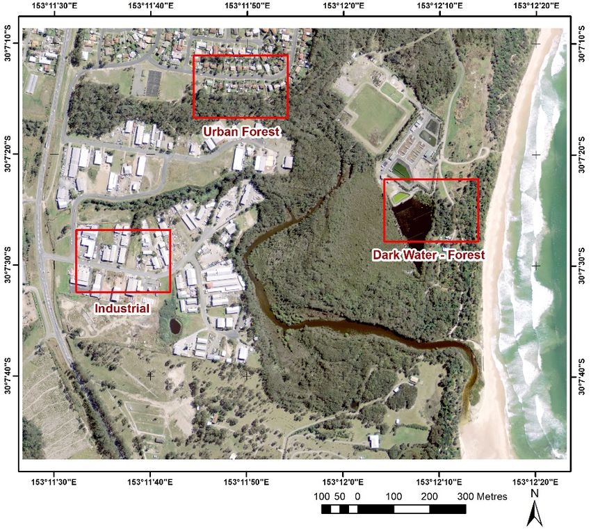
Remote Sens. 2018, 10, 1185                                                                           4 of 21

       Invariant colour models normalise illumination by decoupling pixel responses into intensity
 and colour using RGB colour space transformations. Colour, or ‘colour constancy’ is invariant to
 illumination, while intensity reflects brightness (radiance). These methods exploit the extracted colour,
 hue and intensity information to detect shadow [16,17,25]. In colour aerial imagery, diffuse skylight in
 shadow areas is visually apparent in the colour constant transformation appearing as strong blue-violet
 in colour [25]. The strength of these approaches is that the complexity of illumination is normalised
 from inherent image properties, which avoids corrections using complex physics and scene-specific
 references. Invariant colour models do not overcome atmospheric effects and assume Lambertian
properties for all surface materials.
       Model-based methods require a priori scene surface morphology data and sun-sensor-object
 geometry to delineate shadows. Surface morphology data includes Digital Surface Models (DSMs)
 that are of a spatial scale equal to or better than that of the scene. Shadow is determined by geometric
 calculations, success of these models is reliant on accurate DSM and scene object spatial co-registration.
Also, the models require exact image sun zenith and azimuth angles at image acquisition time.
The advantage of the models is they use DSMs and no spectral information, and so are classified as
 invariant to illumination. The disadvantage is that outputs are a binary mask that have no information
 on abundance of shadow and diffuse skylight.
       Physics-based methods correct for illumination variation by using atmospheric correction,
 sun-object-sensor geometry, terrain and surface material properties to estimate at-ground reflectance
 estimates. To define reflectance, nomenclature from [26] states that reflection is the process where
 electromagnetic flux that is incident on a surface, leaves that surface without a change in wavelength.
 Reflectance is then defined as the fraction of reflected flux from that surface, i.e., out/in. As previously
 mentioned, 6S, ATCOR and FLAASH estimate reflectance from a horizontal surface, with ATCOR
 being the one approach capable of considering topographic or surface material effects. Dymond and
 Shepherd [7] used an algorithm with SPOT 4 imagery corrected to reflectance with 6S and a digital
 elevation model to derive a full topographically corrected image that gives the appearance of being
‘flattened’. Flood, Danaher, Gill and Gillingham [8] extended this work further and introduced surface
 material corrections using BRDFs on Landsat TM/ETM+ and SPOT HRG imagery. Flood, Danaher,
 Gill and Gillingham [8] achieved excellent results by reducing errors due to BRDF by up to 50%.
The advantages of these two approaches are that physics-based information is used to correct for
 illumination. The methods of Flood, Danaher, Gill and Gillingham [8] and Dymond and Shepherd [7]
 are applied to small-scale images with digital elevation models that produce a topographic flattening
 result. However, unlike ATCOR the 6S and FLAASH methods do not consider the blue-skew effects of
 diffuse skylight in umbra, and shadow areas remain.
       Another physics-based approach is the de-shadowing algorithm by Adler-Golden, Matthew,
Anderson, Felde and Gardner [6] applied to an AVIRIS scene atmospherically corrected to reflectance
 using FLAASH. By considering shadow as an endmember, a matched filter vector that considers
 shadow as ‘black’ is used to identify shadow abundance per pixel (shadow fraction). A spectrally
 dependent ratio of direct-to-diffuse illumination is then applied to rebalance the reflectance values.
The shadow fraction is then applied to the rebalanced reflectance data to de-shadow the image.
 Richter and Müller [20] refined the approach to improve estimates of the shadow fraction.
Topographic effects and surface material properties were not applied in these works, but could
 be corrected with a tool such as ATCOR [13]. The derivation of the matched filter vector for shadow
 is constrained to scene-dependent measures, i.e., scene covariance matrix and mean spectral value.
 In a more recent study by Schläpfer, et al. [27] a cast shadow algorithm is used for deriving aerosol
 optical thickness distribution measures to improve atmospheric correction in high-resolution imagery.
The cast shadow algorithm presented considers the diffuse skylight effect by exploiting the scattering
 effect via visible band ratios. The advantages of these methods are that atmospheric corrections and
 diffuse skylight are considered, with excellent results achieved.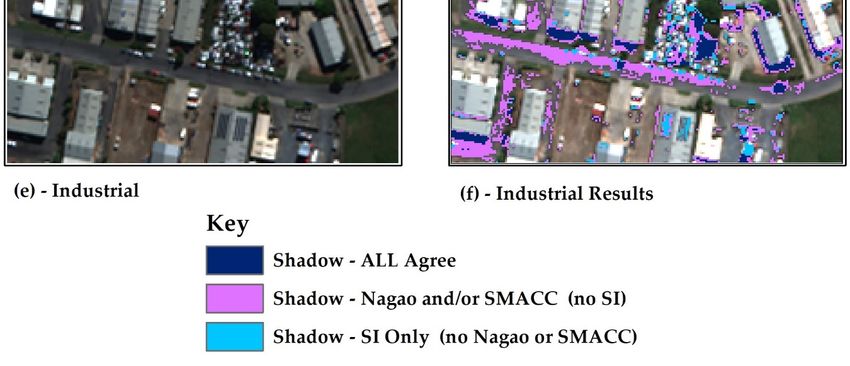
Remote Sens. 2018, 10, 1185                                                                          5 of 21

      Machine learning techniques include supervised and unsupervised classifications.
Supervised classification uses a priori information about surface cover types to generate a
land cover map. User defined training sites (pixels) are selected and assigned to multiple land cover
classes. An algorithm is then applied to assign all other pixels in the image to one of these classes [28].
Unsupervised classification algorithms assign pixels to a user defined number of classes that are
statistically generated without a priori information. Unless both approaches are applied to illumination
corrected data, classification accuracy is wholly reliant on scene resolution and characteristics for
shadow detection, and as such, they are no longer considered.
      In summary, all models possess varying strengths and limitations in their approach to shadow
detection. Property-based approaches work well and have the advantage of not requiring in situ or
ancillary data, but they are scene dependent and require user-specified thresholding. Physics-based
methods address the issue of diffuse skylight but are mostly applied to small-scale imagery that
requires atmospheric correction and ancillary data, such as terrain and sensor BRDF models.
These models are rarely applied to higher-resolution images that possess exponential increases
in scene complexity that require commensurate scale BRDF models and accurately co-registered
terrain data. Model-based methods work well for delineating cast shadow extents where accurate
co-registered terrain information is available but do not measure shadow abundance. Machine learning
techniques are repeatable across varying scales of imagery, but their performance is reliant upon scene
dependency and data dimensionality. An ideal approach to shadow detection should address the
limitations of the discussed models while drawing on the efficiencies and strengths from all.
      The method proposed uses diffuse skylight effect as a surrogate for shadow detection, an approach
that differs to methods that avoid diffuse skylight effects. Diffuse skylight is quantified under clear sky
conditions using a Rayleigh scattering model [29,30] that is converted to a reference vector. All image
pixels are converted to unit vectors, where linear algebra determines the proportion of diffuse skylight
in each pixel using spectral similarity (colour), not intensity. The authors test the hypothesis that
image pixels can have their shadow extent and abundance quantified by the proportion of a diffuse
skylight vector present in each pixel vector. This method uses only vector orientation to delineate
shadow, and thus eliminates the complex physics-based corrections of pixel magnitude associated
with sun-object-scene geometry. Importantly, a unit vector pixel is a linear scaled version of an
original image pixel and the spectral angle does not change post-scaling. This method is invariant to
scene-sensor characteristics, surface material properties and provides a physics-based estimate for
shadow abundance. The method is simple to apply, and is thus beneficial for operational analysis of
high-resolution imagery.
      The method has been implemented using IDL code and Research Systems, Inc. ENVI software,
but the simplicity of the method permits application using just the standard interface tools available in
commercial remote sensing software.

2. Materials and Methods

2.1. Method
     The method proposed here is called Scattering Index (SI) and consists of (1) the creation of a
diffuse skylight vector using a Rayleigh scattering model, (2) normalisation of high-resolution imagery
by conversion to unit vector form, (3) applying vector projection (linear algebra) to quantify proportion
of diffuse skylight ‘colour’ in each normalised image pixel, and (4) defining a threshold for proportion
to determine shadow extent and abundance.
     Diffuse skylight causes a non-linear effect across spectra and is modelled using an exponentially
decreasing function λ−x where the Angstrom-law exponent x determines the relative degree of
scattering for wavelength λ [6,29,31]. The physics principle is that smaller wavelengths are scattered
exponentially more than longer wavelengths.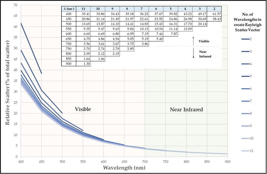
Remote Sens. 2018, 10, 1185                                                                                6 of 21

     The Rayleigh model (λ−4 ) represents scattering in a ‘clear sky’, but the function can be fitted to
varying degrees of sky haze by adjusting the exponent value [29,31]. As the exponent increases from
−4 to 0, scattering across all spectra approaches equality, which is modelled by the zero exponent (λ◦ ).
The Rayleigh model is best suited to images that are atmospherically corrected or where atmospheric
effects are negligible and hence simulate ‘clear sky’.
     The derivation of a diffuse skylight vector is adopted from Chavez [31], which creates a relative
scattering vector, as shown in Equation (2).

                                                          λ i −4
                                               Sλi =               −4
                                                                                                               (2)
                                                       ∑ni=1 λi

where Sλi is the relative percentage of scatter for the ith wavelength, λ = wavelength and n is the total
number of wavelengths.
     Table 1 is an example of a relative Rayleigh scattering model applied to an artificial sensor with
visible and near infrared wavelengths (λ) to create a diffuse skylight vector using Equation (2).

      Table 1. Relative Rayleigh scattering model (λ−4 ) applied to visible and NIR wavelengths. Percentage
      of total scatter is used to create a diffuse skylight vector. A worked example is the Green wavelength
      where 1.22−4 = 0.448 resulting in 0.448/1.756 = 0.26 (or 26%).

            Wavelength (λ nm/Relative             Relative Rayleigh          Rayleigh Scattering Model
                    to Blue)                       Function (λ−4 )              (% of Total Scatter)
             Blue                   (450/1)                 1                            57
            Green                 (550/1.22)              0.448                          26
             Red                  (650/1.44)              0.229                          13
         Near Infrared            (850/1.88)              0.078                          4
                                     Total                1.756

     As shown in Table 1, longer wavelengths have exponentially less scattering, resulting in their
decreased sensitivity to diffuse skylight. Therefore, selection of appropriate wavelengths for a diffuse
skylight vector is crucial and should be restricted to visible wavelengths where sensitivity is measurable.
The sensitivity effect can be observed when varying wavelength ranges are applied to the Rayleigh
model. This is shown in Figure 3 using 50 nm wavelength increments across the visible-NIR spectrum.
     The inclusion of longer wavelengths reduces the relative scatter of shorter wavelengths, with the
converse also being true. A similar trait exists for the diffuse skylight signature, where inclusion of
longer wavelengths produces a ‘flatter’ signature and lower overall scatter range, whereas exclusion
of long wavelengths increases the signature curve and total scatter range. In applying the Rayleigh
model to a sensor, the centres of the band wavelength ranges define the diffuse skylight vector.
     Image pixels are represented as vectors in n-dimensional spectral space. In vector representation,
two characteristics can uniquely describe any pixel, orientation (colour) and magnitude (intensity).
Obtaining a single measure for magnitude is simple using Pythagoras’ theorem, but a single measure
for orientation is exponentially more complex due to the multiple reference axes. To alleviate this
complexity, colour can be represented by a normalised image pixel vector. Normalisation using an
invariant colour model approach has been applied for two reasons, (1) to aid visual detection of diffuse
skylight, and (2) to simplify the linear algebra formulation as per Equation (3)
                                                          *
                                                           p
                                                   p̂ =   *                                                    (3)
                                                           p

                              *
where p̂ is unit vector, p is pixel vector and ||p̂|| is the pixel vector magnitude. Unit vector magnitude
||p̂|| is always 1.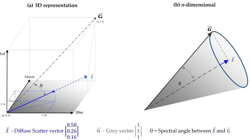
= (2)
∑
where is the relative percentage of scatter for the ith wavelength, λ = wavelength and n is the
total number of wavelengths.
Remote Sens. 2018, 10, 1185 7 of 21
Table 1 is an example of a relative Rayleigh scattering model applied to an artificial sensor with
visible and near infrared wavelengths (λ) to create a diffuse skylight vector using Equation (2).
When pixel vector magnitude is normalised to one, then pixel signatures are represented as shape
only Table
and can 1. Relative Rayleigh
be compared scattering
directly. model (λ−4) applied
Furthermore, magnitudeto visible
is a and NIR wavelengths.
continuum, Percentage
and its use for shadow
of total scatter is used to create a diffuse skylight vector. A worked example is the
detection relies upon user or scene specific ‘dark pixel’ thresholding. This method uses only vectorGreen wavelength
where 1.22
orientation
−4 = 0.448 resulting in 0.448/1.756 = 0.26 (or 26%).
to delineate shadow. Importantly, a unit vector pixel is a linear scaled version of an original
image pixel and the spectral angle does not change post-scaling. Rayleigh Scattering
Relative
Wavelength (
The spectral angle between any two vectorsRayleigh is determined byModel the spectral angle Equation (4)
(% of Total
nm/Relative to Blue)
Function
(λ )−4 Scatter)
n
Blue (450/1) 1 ∑ s i p 57
θ(s,p) = Cos−1 q i=1q i , (4)
Green (550/1.22) 0.448 26
∑ni=1 s2i · ∑ni=1 p2i
Red (650/1.44) 0.229 13
Near Infrared (850/1.88) 0.078
where θ is spectral angle, s is the ith band value of the Rayleigh scatter vector, 4 p is the ith value of the
pixel band and n is number of bands. Total 1.756
The spectral angle θ(s,p) is not necessary to determine proportion because the term of equation [4]
Asparentheses
inside shown in Table
is the 1, longer
linear wavelengths
algebra formula have exponentially
for vector projection,less
i.e.,scattering,
how muchresulting
of p is s,in
ortheir
vice
decreased
versa. The sensitivity
relationshiptois
diffuse
shownskylight. Therefore,
in Equation (5) selection of appropriate wavelengths for a diffuse
skylight vector is crucial and should be restricted to visible wavelengths where sensitivity is
measurable. The sensitivity effect can beVP (s,p) = Cosθ
observed when ),
(s,pvarying wavelength ranges are applied(5) to
the Rayleigh model. This is shown in Figure 3 using 50 nm wavelength increments across the visible-
where VP is the vector projection s in p. VP value range is 0–1.
NIR spectrum.
Figure 3.3.Rayleigh
Figure Rayleigh scatter
scatter vector
vector signatures
signatures across across theand
the visible visible and near
near infrared infrared
spectrum spectrum
wavelengths.
wavelengths. Signature variation is caused by increasing or decreasing the number of wavelengths
Signature variation is caused by increasing or decreasing the number of wavelengths used to derive
used
the to derive
Rayleigh the Rayleigh
scatter vector. scatter vector.
The inclusion of longer wavelengths reduces the relative scatter of shorter wavelengths, with
From linear algebra, VP(s,p) has a value range from 0 to 1, where 0 is an orthogonal vector and 1
the converse also being true. A similar trait exists for the diffuse skylight signature, where inclusion
is a collinear vector. Equation (5) is used to determine the proportion of diffuse skylight vector in each
pixel vector and a threshold value in the 0–1 range is required to define shadow extent.
Here we adopt a diffuse skylight threshold that is independent of illumination variations and
scene characteristics. If the diffuse scattering effect was non-existent, then shadow could be truly
defined as ‘black’ and in vector form, this would mean collinearity with a grey vector where all spectra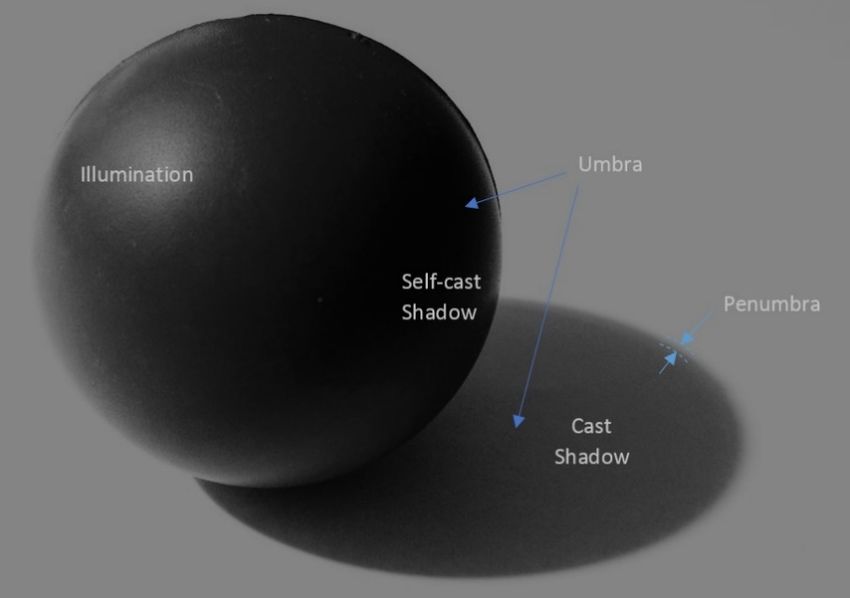
Remote Sens. 2018, 10, 1185                                                                                         8 of 21

are equal and zero. Because we use diffuse skylight to define shadow, the proportion of shadow is
commensurate with an angular rotation of theta away from the grey vector towards the diffuse scatter
vector. Figure 4 illustrates this using a simple 3-band image example of a Rayleigh scatter vector and a
simple  visualisation
Remote Sens. 2018, 10, x FOR  n-dimensions.
                          forPEER REVIEW                                                            8 of 20

      Figure 4.
      Figure   4. 3D
                  3D example
                      example showing
                                 showing thethe spectral
                                                spectral angle
                                                         angle rotation
                                                               rotation θθ from
                                                                            from grey
                                                                                 grey vector
                                                                                      vector to
                                                                                              to aa 3-band
                                                                                                     3-band Rayleigh
                                                                                                             Rayleigh
      scatter vector. (a) Is a 3D visualisation of the relationship between grey vector and diffuse scatter scatter
      scatter  vector.  (a) Is a  3D  visualisation of the relationship  between   grey vector   and   diffuse vector
      vector
      and  (b)and  (b) an equivalent
               an equivalent            for n-dimensions
                                for n-dimensions   withoutwithout   theshown.
                                                            the n axis  n axis shown.

       The spectral angle between a Rayleigh diffuse skylight vector *           ( ) and the grey vector (* ) defines
      The spectral angle between a Rayleigh diffuse skylight vector ( s ) and the grey vector ( g ) defines
the radial distance between diffuse skylight and true black shadow respectively. This distance is
the radial distance between diffuse skylight and true black shadow respectively. This distance is
defined as vector proportion (            ) using Equation (5) and is used as the threshold to delineate
defined as vector proportion (VP((s,g, ))) using Equation (5) and is used as the threshold to delineate
shadow extent and abundance i.e., all pixels within θ are shadowed.
shadow extent and abundance i.e., all pixels within θ are shadowed.
       First, we simplify (5) by substituting the unit vector image
      First, we simplify (5) by substituting the unit vector image
                                                                 .
                                                        = *                                                      (6)
                                                           p̂||· s||
                                                  SIp =                                                           (6)
                                                           ||s||
where          (Scatter Index) is proportion of skylight in pixel p.              is the unit vector form of image
pixels,SIp is
where          the diffuse
             (Scatter      skylight
                      Index)         vector of
                             is proportion  and  || || isinmagnitude
                                               skylight       pixel p. p̂ isofthe
                                                                               theunit
                                                                                    diffuse skylight
                                                                                        vector       vector.
                                                                                               form of image pixels,
*      We  finalise the method   (7) by confining  Equation        (6) to the threshold   for shadow  pixels
 s is the diffuse skylight vector and ||s|| is magnitude of the diffuse skylight vector.
      We finalise the method (7) by confining .
                                         = Equation
                                           ( , ), for (6) to≥the threshold for shadow pixels
                                                                 ( , )        ( , ),                                    (7)
                                                    || ||
                                                      *
where           is proportion or abundance  p̂· s
            ( , )                 SI(p,a) = of shadow
                                                  , for SI(in  each shadowed pixel.
                                                            p,a) ≥ VP(s,g) ,                       (7)
                                            ||s||
Method Comparison
where SI(p,a) is proportion or abundance of shadow in each shadowed pixel.
      The SI shadow detection method is evaluated against the SMACC (Spectral Maximum Angle
Method
Convex Comparison
          Cone) detection algorithm [32] and Nagao’s histogram threshold on image brightness [24].
The methods are applied to both Worldview-3 imagery corrected to the bottom of atmosphere
     The SI shadow detection method is evaluated against the SMACC (Spectral Maximum Angle
reflectance [26] using FLAASH and non-reflectance ADS40 airborne imagery in 8-bit DN values.
Convex Cone) detection algorithm [32] and Nagao’s histogram threshold on image brightness [24].
      Both SMACC and Nagao methods were assessed in a comprehensive review by Adeline, Chen,
The methods are applied to both Worldview-3 imagery corrected to the bottom of atmosphere
Briottet, Pang and Paparoditis [21], where Nagao’s method proved overall best with an F-score
reflectance [26] using FLAASH and non-reflectance ADS40 airborne imagery in 8-bit DN values.
average of 92.5, and SMACC proved less effective with an average F-score of 83.9. The shadow
     Both SMACC and Nagao methods were assessed in a comprehensive review by Adeline, Chen,
detection approach of Richter and Müller [20] was the second-best performer (average F-score 90),
Briottet, Pang and Paparoditis [21], where Nagao’s method proved overall best with an F-score average
but requires one band from the near infrared and two bands from shortwave infrared, which excludes
both ADS40 and Worldview-3 sensors. SMACC is the second option because it is a physics-based
approach, it is an automated tool in ENVI software and shadow is referenced as a ‘black’ vector as
per the physics-based approach of Richter and Müller [20]
      SMACC analysis was run using 30 endmembers and a ‘positive only’ constraint that produces a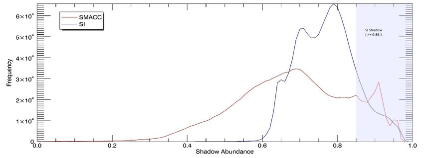
Remote Sens. 2018, 10, 1185                                                                                  9 of 21

of 92.5, and SMACC proved less effective with an average F-score of 83.9. The shadow detection
approach of Richter and Müller [20] was the second-best performer (average F-score 90), but requires
one band from the near infrared and two bands from shortwave infrared, which excludes both ADS40
and Worldview-3 sensors. SMACC is the second option because it is a physics-based approach, it is an
automated tool in ENVI software and shadow is referenced as a ‘black’ vector as per the physics-based
approach of Richter and Müller [20]
      SMACC analysis was run using 30 endmembers and a ‘positive only’ constraint that produces
a fractional abundance of shadow per pixel. For Worldview-3 imagery, this is directly comparable
with the SI method in terms of shadow abundance. However, the ADS40 imagery was corrected to
reflectance, resulting in the histogram of shadow abundance being left skewed and thus nullifying the
use of the SI threshold for SMACC. Instead, for the SMACC method, we implemented a supervised
threshold based on Otsu [33] on the ADS40 abundance image to create a binary mask and offset the
histogram skew. Therefore, for the purposes of this paper, we could only compare abundances for the
Worldview image subsets.
      To generate the Nagao shadow mask, original images were smoothed using a 5 × 5 pixel window
as per the edge-preserving smoothing algorithm of Nagao and Matsuyama [34]. A brightness or
intensity grey level image is derived from the smoothed image that had a grey level threshold
applied in ENVI software using the Otsu [33] histogram thresholding parameter to finalise the mask.
The Worldview-3 image has eight bands, so the blue, green, red and NIR1 bands were selected to
replicate Nagao’s method.
      To compare performance on different sensors the methods were applied to high-resolution
imagery from the airborne ADS40 sensor (DN values) and spaceborne Worldview-3 imagery corrected
to reflectance using FLAASH after MODTRAN [12]. The diffuse skylight vector (λ−4 ) was created
from the centres of all spectral bands in the visible spectrum for both images. The angles between the
diffuse skylight and grey vectors were used as shadow thresholds and shown as both degrees and
vector proportion in Table 2.

          Table 2. Diffuse skylight vectors and SI shadow thresholds for ADS40 and Worldview images.

                                                                                        SI THRESHOLD
      Image           Visible Bands Used   Diffuse Skylight Vector (λ−4 )
                                                                                 Degrees (◦ )   Proportion VP(s,g)
     ADS40                      1,2,3             [0.577, 0.263, 0.159]             28.10             0.89
   Worldview-3                1,2,3,4,5    [0.418, 0.261, 0.148, 0.099, 0.071]      32.43             0.85

2.2. Materials
     All analyses were performed on a common extent for images from the airborne Leica ADS40
and spaceborne Worldview-3 satellite sensors. The image scene was of an area 1513 × 1196 m on the
southern limits of the Woolgoolga township on the mid north coast of New South Wales, Australia.
The scene centre is located by coordinates 153◦ 110 55 E and 30◦ 70 27 S. The scene consists of urban,
industrial, cleared grassland, sewage treatment plant, horticulture, ocean, beach, sealed/unsealed
roads, littoral rainforest, heath and wet/dry sclerophyll eucalypt forest. Three subsets of equal size
(260 × 170 m) were selected for evaluation as they vary and contain targets known for misclassification
of shadow. Both Worldview-3 and ADS40 images and the selected subsets ‘Urban Forest’, ‘Dark
Water-Forest’ and ‘Industrial’ are shown in Figure 5.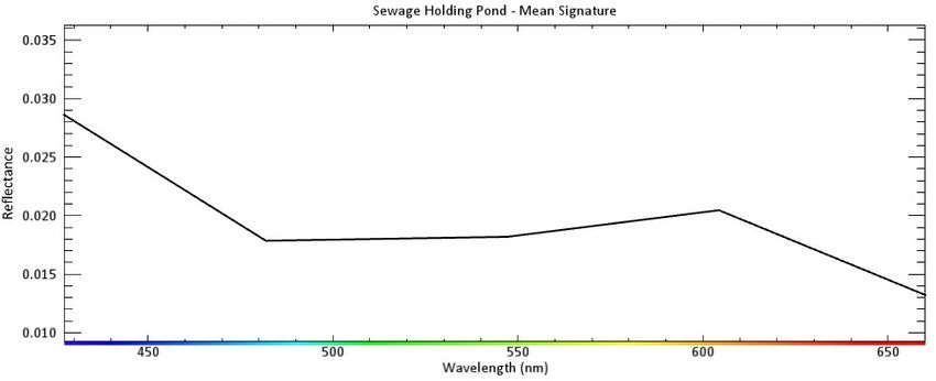
imagery is part of the New South Wales state government’s Land & Property Information (LPI)
Standard Coverage Imagery Capture Program [36]. The colour/near infra-red four-band imagery
(428–492 nm, 533–587 nm, 608–662 nm, 833–887 nm) was captured using a Leica ADS40 sensor with
resultant 50 cm ground sampling distance. Processing included ortho-rectification, colour-matching
and the
Remote   joining
       Sens.        of1185
             2018, 10, overlapping image strips. No atmospheric correction procedures were applied, and
                                                                                                 10 of 21
image values are 8-bit DN.

Remote Sens. 2018, 10, x FOR PEER REVIEW                                                                  11 of 20
                                                      (a)

                                                      (b)
     Figure 5. Study
     Figure 5. Studyarea
                      areashowing
                            showing images
                                  images andand target
                                             target    subset
                                                    subset     areas.
                                                           areas.      (a) ADS40
                                                                  (a) ADS40       image,
                                                                             image,        (b) Worldview-3
                                                                                     (b) Worldview-3  image.
     image. Urban Forest,
     Urban Forest,         Dark Water-Forest
                   Dark Water-Forest         and Industrial
                                      and Industrial subsets subsets
                                                             are usedare
                                                                       forused for shadow
                                                                           shadow           target detection
                                                                                    target detection and are
     and arein
     shown   shown
               red. in red.

2.3. Performance Comparison
     Most shadow detection performance measures have been applied using an independent pre-
analysis shadow extent boundary [17]. Here we have used a post-analysis approach that targets
shadow detection anomalies. For shadow extent, Overall Accuracy and F-Scores are used to quantify
performance, after Adeline, Chen, Briottet, Pang and Paparoditis [21]. Table 4 shows the formulation
of Overall Accuracy and F-Scores [37].
Remote Sens. 2018, 10, 1185 11 of 21
The Worldview-3 image was acquired under clear-sky conditions (visibility > 100 km) on 4th April,
2016 at 10:07 am (Australian Eastern Standard Time) with sun azimuth and zenith angles of 28◦ 240 0600
and 36◦ 030 3800 , respectively. The image was acquired in panchromatic and eight multispectral bands,
but only the multispectral bands were used for shadow detection. The spatial resolution was 1.2 metre
ground separation distance, with sensor bands and their centres shown in Table 3.
Table 3. Worldview-3 sensor bands showing bandwidths and their wavelength centres in nanometres.
Worldview-3 Bands λ (nm) λ Centre
1 Coastal 400–452 426
2 Blue 448–510 479
3 Green 518–586 552
4 Yellow 590–630 610
5 Red 632–692 662
6 RedEdge 706–746 726
7 NIR1 770–895 832.5
8 NIR2 860–1040 950
Worldview-3 Imagery was supplied as DN values that were converted to top of atmosphere
radiance by applying supplied gains and offsets to each pixel digital number. Top of atmosphere
radiance was then converted to reflectance using ENVI’s FLAASH atmospheric correction module
after MODTRAN 5 [35] using a scene average elevation of 113 m above sea level calculated from
LiDAR data.
The ADS40 imagery was acquired on the 11th of September 2009 at 0945 h (Australian Eastern
Standard Time) with sun azimuth and zenith angles as 41◦ 460 2400 and 46◦ 320 2800 respectively.
The imagery is part of the New South Wales state government’s Land & Property Information
(LPI) Standard Coverage Imagery Capture Program [36]. The colour/near infra-red four-band imagery
(428–492 nm, 533–587 nm, 608–662 nm, 833–887 nm) was captured using a Leica ADS40 sensor with
resultant 50 cm ground sampling distance. Processing included ortho-rectification, colour-matching
and the joining of overlapping image strips. No atmospheric correction procedures were applied, and
image values are 8-bit DN.
2.3. Performance Comparison
Most shadow detection performance measures have been applied using an independent
pre-analysis shadow extent boundary [17]. Here we have used a post-analysis approach that targets
shadow detection anomalies. For shadow extent, Overall Accuracy and F-Scores are used to quantify
performance, after Adeline, Chen, Briottet, Pang and Paparoditis [21]. Table 4 shows the formulation
of Overall Accuracy and F-Scores [37].
Table 4. Formulation for overall accuracy and F-score.
Predicted Positive Predicted Negative
Reference Positive TP FN
Reference Negative FP TN
Precision (P) = TPTP
+FP
Recall (R) = TPTP
+FN
TP+TN
Overall Accuracy = TP+FP +TN +FN
R× P
F − score = 2 × R+ PRemote Sens. 2018, 10, 1185 12 of 21
In this post-analysis approach, reference points are created within a shadow extent created by
combining shadow masks from all three detection methods. The method is described stepwise,
as follows:
1. Convert binary shadow masks (1 = Shadow, 0 = No shadow) from all three methods to vector
polygons maintaining pixel edge boundaries, i.e., unsmoothed conversion.
2. Spatially combine all three binary shadow masks to create eight unique classes, i.e., all agree
non-shadow, only SI shadow, only SMACC shadow, only Nagao shadow, SI & SMACC shadow,
Nagao & SMACC shadow and SI & Nagao shadow.
3. Remove ‘all agree no shadow’ class, as no statistical power is gained from its inclusion.
4. Create a dataset of point references using a stratified random sampling strategy using the
remaining seven classes as strata.
5. The number of points per class is determined by the ratio of total class area to the number of
polygons in the class. The ratio is then doubled to approximate a binomial distribution sample
size of N = 76 based on an expected map accuracy of 95% and allowable error of 5% [26].
6. Using original images only, perform an independent visual assessment of all reference points
and assign values 1 for shadow and −1 for non-shadow. Importantly, shadow value 1 captures
self-cast and cast shadow areas.
7. Overlay reference points with each method’s shadow mask and determine F-Score and
Overall Accuracies.
Table 5 shows the overall counts and shadow versus non-shadow assignments for reference points
from the three subsets in both images
Table 5. Counts of shadow/non-shadow reference points used in image subsets for Worldview-3
and ADS40.
Worldview-3 ADS 40
Subsets Non-Shadow Non-Shadow
Shadow (1) Total Points Shadow (1) Total Points
(−1) (−1)
Urban
74 35 109 73 8 81
Forest
Dark
35 65 100 52 106 158
Water-Forest
Industrial 75 25 100 128 10 138
For shadow abundance, it is logistically difficult to obtain physics-based reference data that is
both synchronised to image acquisition and sun/sensor geometry. Evaluation of shadow abundance
can only be performed on Worldview subsets and is done by visual comparison between the SI and
SMACC methods. Comparison is done using histograms created from shadow pixels regarded as
shadow by both SI and SMACC methods.
3. Results
Shadow Extent
Table 6 provides the results for Overall Accuracies and includes the mean for each method for
both ADS40 and Worldview-3 images. The mean of Overall Accuracies for each image subset is
included and shows that shadow detection for Urban Forest and Industrial subsets is similar (70.9%
and 76.7% respectively) and the Dark Water Forest subset is significantly lower (50.5%).Remote Sens. 2018, 10, 1185 13 of 21
Table 6. Overall accuracy results for all three methods on both ADS40 and Worldview-3 images that
includes method mean and image subset mean.
Worldview-3 ADS 40 Image Subset
Image Subset
SI Nagao SMACC SI Nagao SMACC Mean
Industrial 79.0 79.0 69.0 87.0 79.0 67.4 76.7
Urban Forest 82.4 67.0 62.4 70.4 74.1 69.1 70.9
Dark Water – Forest 70.0 46.0 41.0 86.7 34.8 24.7 50.5
Method Mean 77.1 64.0 57.5 81.3 62.6 53.7
Table 7 provides F-score results in same format as Table 6. Table 8 is the final Overall Accuracy
ranking and Table 9 is the final F-score rankings. These rankings are the means of Method Mean from
both images. For example, in Table 8 the SI score of 79.2 is the mean of the SI Method Mean scores
(77.1 and 81.3) from Table 6.
Table 7. F-score results for all three methods on both ADS40 and Worldview-3 images that includes
method mean and image subset mean.
Worldview-3 ADS 40 Image Subset
Image Subset
SI Nagao SMACC SI Nagao SMACC Mean
Industrial 85.7 85.3 80.0 92.6 87.6 79.8 85.2
Urban Forest 88.7 77.5 74.2 81.0 84.4 80.0 81.0
Dark Water – Forest 68.8 50.9 43.8 76.9 47.2 32.8 53.4
Method Mean 81.1 71.2 66.0 83.5 73.1 64.2
Table 8. Final rankings for Overall Accuracy calculated from Method Mean in Table 6.
Final Ranking (Overall Accuracy)
SI 79.2
Nagao 63.3
SMACC 55.6
Table 9. Final rankings for F-score calculated from Method Mean in Table 7.
Overall Ranking (F-Score)
SI 82.3
Nagao 72.1
SMACC 65.1
Figure 6 displays the results for the ADS40 image subsets using three class display shown in the
figure key. The three classes are (1) all three methods agree there is shadow, (2) only Nagao or SMACC
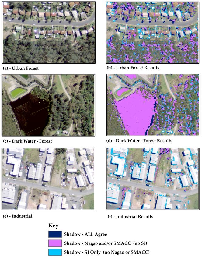
detect shadow, and (3) only SI detects shadow. Figure 7 displays the results for Worldview-3 image
subsets with the same key from Figure 6.Remote Sens. 2018, 10, 1185 14 of 21
Remote Sens. 2018, 10, x FOR PEER REVIEW 14 of 20
6. Shadow
Figure 6. Shadow detection results for ADS40
ADS40 image
image subsets.
subsets. Binary shadow masks from SI, Nagao
Nagao
and SMACC methods are combined into three display classes. Subsets (a,c,e) are original images and
subsets (b,d,f) are respective
respective shadow
shadow detection
detection results.
results.Remote Sens. 2018, 10, 1185 15 of 21
Remote Sens. 2018, 10, x FOR PEER REVIEW 15 of 20
Figure 7.7. Shadow
Figure Shadow detection
detection results
results for
for Worldview-3
Worldview-3 image
image subsets.
subsets. Binary shadow masks from SI, SI,
Nagao
NagaoandandSMACC
SMACC methods
methodsareare
combined
combinedinto into
threethree
display classes.
display Subsets
classes. (a,c,e) are
Subsets original
(a,c,e) images
are original
and subsets
images and (b,d,f)
subsetsare respective
(b,d,f) shadow shadow
are respective detectiondetection
results. results.
The fraction
The fraction of
of shadow
shadow abundance
abundance in in aa pixel
pixel is
is only
only produced
produced byby SISI and
and SMACC
SMACC methods
methods so
so
theirabundance
their abundancehistograms
histogramsare
areused
usedfor
forcomparison.
comparison.FigureFigure 8 below
8 below is for
is for SI SI v SMACC
v SMACC comparison
comparison of
of shadow abundance in ADS40 where the shaded area indicates SI shadow as per threshold (≥0.89)
for ADS40 imagery in Table 2.
Figure 9 is the same format as Figure 8 using Worldview-3 imagery.Remote Sens. 2018, 10, 1185 16 of 21
shadow abundance in ADS40 where the shaded area indicates SI shadow as per threshold (≥0.89) for
Remote Sens.
ADS40 2018, 10,inx Table
imagery FOR PEER
2. REVIEW 16 of 20
Remote Sens. 2018, 10, x FOR PEER REVIEW 16 of 20
Figure
Figure 8.
8. Shadow
Shadow abundance
abundance comparison
comparison between
between SI
SI and
and SMACC
SMACC shadow
shadow detection
detection methods
methods applied
applied
to ADS40 imagery. Shaded area indicates SI threshold range (≥0.89) for shadow.
to ADS40 imagery. Shaded area indicates SI threshold range (≥0.89) for shadow.
Figure 8. Shadow abundance comparison between SI and SMACC shadow detection methods applied
Figure 9 is
to ADS40 the same
imagery. format
Shaded asindicates
area Figure 8SIusing Worldview-3
threshold imagery.
range (≥0.89) for shadow.
Figure 9. Shadow abundance comparison between SI and SMACC shadow detection methods applied
to Worldview-3 imagery. Shaded area indicates SI threshold range (≥0.85) for shadow.
Figure 9. Shadow abundance comparison between SI and SMACC shadow detection methods applied
Figure 9. Shadow abundance comparison between SI and SMACC shadow detection methods applied
4. Discussion
Worldview-3 imagery.
to Worldview-3 imagery.Shaded
Shadedarea
areaindicates
indicatesSI
SIthreshold
thresholdrange
range((≥0.85)
≥0.85) for shadow.
shadow.
The results for the three methods in the Overall Accuracy from Table 8 show separation of
4. Discussion
performance
4. Discussionwith measures of 79.2%, 63.3% and 55.6% for SI, Nagao and SMACC respectively. SI is
best performer with a 15.9% improvement on Nagao, followed by SMACC with 7.7% below that of
The results
The results for
for the
the three
three methods
methods in in the
the Overall
Overall Accuracy
Accuracy from Table 88 show
from Table show separation
separation of of
Nagao. The order of performance and degree of separation is similar for F-scores in Table 9 with
performance with measures of 79.2%, 63.3% and 55.6% for SI, Nagao and
performance with measures of 79.2%, 63.3% and 55.6% for SI, Nagao and SMACC respectively. SI is SMACC respectively. SI is
results of 82.3, 72.1 and 65.1 for SI, Nagao and SMACC respectively. Differences in F-scores show
best performer
best performer withwith aa 15.9%
15.9% improvement
improvement on on Nagao,
Nagao, followed
followed by by SMACC
SMACC with with 7.7%
7.7% below
below that
that of
of
separation of 10.2 between SI and Nagao and 7.0 separating Nagao and SMACC. For all methods, the
Nagao. The
Nagao. The order
order ofof performance
performance and and degree
degree of of separation
separation is is similar
similar forfor F-scores
F-scores in in Table
Table 99 with
with
overall performance shows an F-score range of 82.3–65.1 compared to the review by Adeline, Chen,
results of
results of 82.3,
82.3, 72.1
72.1 and
and 65.1
65.1 for
for SI,
SI, Nagao
Nagao and and SMACC
SMACC respectively.
respectively. Differences
Differences inin F-scores
F-scores show
show
Briottet, Pang and Paparoditis [21], which reported an F-score-range of 92.5–83.9. In the review by
separation of
separation of 10.2
10.2between
betweenSISIand andNagao
Nagaoand and7.07.0
separating
separating Nagao
Nagao andandSMACC.
SMACC. ForForall methods, the
all methods,
Sanin, Sanderson and Lovell [17], a mean of two detections, foreground object and shadow, resulted
overall performance shows an F-score range of 82.3–65.1 compared to the
the overall performance shows an F-score range of 82.3–65.1 compared to the review by Adeline, review by Adeline, Chen,
in a score range of 90–65 using the Recall measure shown in Table 4. In both reviews, the cast shadow
Briottet,
Chen, Pang and
Briottet, PangPaparoditis [21], which
and Paparoditis reported
[21], which an F-score-range
reported an F-score-range of 92.5–83.9. In the
of 92.5–83.9. review
In the reviewby
references used to measure performance are generated prior to analysis. The performance measure
Sanin,
by Sanderson
Sanin, Sanderson andandLovell [17],
Lovell a mean
[17], a mean ofof
twotwodetections,
detections,foreground
foregroundobjectobjectand
andshadow,
shadow, resulted
resulted
in this paper, the stratified random sampling strategy, is applied post-analysis and provides three
in a score range of 90–65 using the Recall measure shown in Table 4. In both reviews, the cast shadow
in a score range of 90–65 using the Recall measure shown in Table 4. In both reviews, the cast shadow
important properties: (1) there is replication of strata, (2) replication increases probability of capturing
references used
references used toto measure
measure performance
performance are are generated
generated prior
prior toto analysis.
analysis. TheThe performance
performance measure
measure
both cast and self-cast shadow, and (3) references get located on features that are problematic for
in this
in this paper,
paper, thethe stratified
stratified random
random sampling
sampling strategy,
strategy, isis applied
applied post-analysis
post-analysis andand provides
provides three
three
shadow detection. The lower performance range of 82.3–65.1 reflects the increased rigour in the
important properties: (1) there is replication of strata, (2) replication increases probability
important properties: (1) there is replication of strata, (2) replication increases probability of capturing of capturing
performance measure used. Therefore, with the design of performance measures considered, the SI
both cast and self-cast shadow, and (3) references get located on features that are problematic for
method is the best performing shadow detection method followed by Nagao and SMACC
shadow detection. The lower performance range of 82.3–65.1 reflects the increased rigour in the
respectively.
performance measure used. Therefore, with the design of performance measures considered, the SI
The mean Overall Accuracies and F-scores for all subsets in both images are shown in Tables 6
method is the best performing shadow detection method followed by Nagao and SMACC
and 7. Again, SI performed better in all subsets in both images followed by Nagao and SMACC
respectively.Remote Sens. 2018, 10, 1185 17 of 21
both cast and self-cast shadow, and (3) references get located on features that are problematic for
shadow detection. The lower performance range of 82.3–65.1 reflects the increased rigour in the
performance measure used. Therefore, with the design of performance measures considered, the SI
method is the best performing shadow detection method followed by Nagao and SMACC respectively.
The mean Overall Accuracies and F-scores for all subsets in both images are shown in Tables 6
and 7. Again, SI performed better in all subsets in both images followed by Nagao and SMACC
respectively. In all six subsets measured, the SI method outperformed all others with one exception.
Nagao outperformed SI in the ‘Urban Forest’ subset in ADS40 imagery with small Overall Accuracy
and F-score separations of 3.5 and 3.7 respectively. The only variable is the ADS40 imagery, so it cannot
be deduced that Nagao’s method is overall better-performing across the ‘Urban Forest’ subsets.
For the SI and SMACC methods only, the abundance of shadow in each pixel is graphically shown
in Figures 8 and 9 by comparing the histograms of abundance outputs for ADS40 and Worldview-3
images, respectively. For an illuminated image with a relatively high sun-sensor angle and minimal
terrain effects, most pixels will be shadow free resulting in a minority of shadow pixels. Under the same
image conditions, an ideal histogram of shadow abundance would have a minimum shadow threshold
located at the far right of the abundance axis (x axis) with low pixel counts above that threshold.
This pattern is observed in Figures 8 and 9, highlighted by the SI thresholds shown as shaded
areas. The ADS40 histograms in Figure 8 show the SMACC histogram (red line) has a left-skewed
distribution. All other abundances in both figures reflect a right-skewed distribution. The left-skewed
ADS40 histogram highlights the scene-sensor dependency of the SMACC algorithm [6,20]. The SMACC
algorithm treats shadow as a ‘null’ or ‘black’ vector and its abundance in a pixel relies upon the resulting
linear combination of all endmembers in that pixel [32]. With SMACC, endmembers are selected from
n-dimensional data space and the four band ADS40 imagery has low dimensionality, resulting in poor
shadow abundance estimates. The SI method is invariant to scene-sensor characteristics and provides
a physics-based estimate for shadow abundance.
The image subsets are selected to target shadow detection difficulties with comparative results
of their subset means provided in Tables 6 and 7. The ‘Industrial’ subset (F-score 85.2) is dominated
by homogeneous human structures that are impervious and produce cast shadows of high contrast.
The ‘Urban forest’ subset (F-score 81.0) combines this with natural schlerophyll forest containing
cast and self-cast shadows and the ‘Dark Water Forest’ subset (F-score 53.4) is mostly water and
schlerophyll forest. From both Overall Accuracy and F-scores, shadow detection accuracy improves
on scenes dominated by human structures and performance reduces with the increased heterogeneity
of natural landscapes.
The SI method detects finer shadow detail and discriminates between dark and naturally dark
objects as seen by the sky-blue symbol colour in the higher resolution ADS40 imagery (50 cm)
shown in Figure 6. Examples of finer shadow detection are backyard fence shadows (Figure 6b),
car shadows (Figure 6b,c) and factory building shadows (Figure 6f) that are missed by Nagao and
SMACC. SI excludes some schlerophyll forest shadowing in the ‘Urban Forest’ subset (Figure 6b),
explaining the better F-score and accuracy for Nagao for that subset. However, SI detects both
self-cast tree shadows in forest and house shadows (Figure 6d) where Nagao and SMACC do not.
Detection errors for both Nagao and SMACC are of the dark water body and sewage holding ponds in
Figure 6d. Nagao selects the dark water body because it is low intensity and SMACC assumes a ‘black’
vector because of similar low values in all bands. SI uses diffuse skylight colour and that ignores the
naturally dark body because of a low proportion (Remote Sens. 2018, 10, 1185 18 of 21
in Figure 7c, where there is an increase in aquatic vegetation cover on the dark water body and one
sewage holding pond is mostly evaporated. In the ‘Urban Forest’ subset (Figure 7b), SI detects both
forest and tree crown shadows with low agreement from Nagao and SMACC. All three methods
incorrectly detect the grey bitumen road and residential houses. Nagao and SMACC detect all the
bitumen road and all houses with darker roofing, reinforcing the limitations of using intensity and
the ‘black’
Remote vector.
Sens. 2018, 10, xSI
FORerrors
PEERare minor in comparison with detection of one blue house roof (middle
REVIEW 18 of 20
left, Figure 7b) and a small portion of the bitumen road, shown as ‘All Agree’ in the top right corner
(Figure 7b). by
is detected A similar
Nagao scenario
and SMACC.occursSIon thenot
does ‘Industrial’ subset (Figure
detect bitumen but does 7f), where
detect grey bitumen
pitches of factoryroad is
roofs
detected
that havebyreduced
Nagao and SMACC. because
illumination SI does notthe detect
pixels bitumen
present as butdiffuse
does detect pitches
skylight. of factory
In the roofs
‘Dark Water
that have
Forest’ reduced
subset illumination
(Figure 7d), Nagaobecause
and the
SMACCpixelsdetect
presentallasthe
diffuse
darkerskylight.
portions In the ‘Dark body
of water Wateraquatic
Forest’
subset (Figure
vegetation 7d), Nagao
where SI detects andonly
SMACC detect allportions.
the darkest the darkerThe portions
sewageofholding
water bodypondaquatic
in thevegetation
top of the
where
subsetSIis detects
very dark onlyand thealldarkest portions.
detect this The sewage
as shadow. holding
For SI, this is notpond in thebecause
an error, top of the
the subset
sensor is very
detects
dark and all detect this as shadow. For SI, this is not an error, because the sensor
a small diffuse skylight response over a very dark body due to its very low radiance. This is shown detects a small diffuse
skylight
in Figureresponse
10 usingover a very dark
a spectral bodyfor
signature duetheto holding
its very low
pond radiance.
derivedThisfromistheshown
meanin of
Figure 10 using
all pixels and
avisible
spectral signature
bands. for the holding pond derived from the mean of all pixels and visible bands.
Figure10.
Figure 10.Mean
Meanspectral
spectral signature
signature of aof a dark
dark holding
holding pondthe
pond from from the wavelength
visible visible wavelength bands
bands showing
showing
low low reflectance
reflectance values andvalues
higherand higher
blue blue wavelength
wavelength response. response.
The SI method detects bodies that contain or present with diffuse skylight effects but is not an
The SI method detects bodies that contain or present with diffuse skylight effects but is not an
error of commission. Shadow detection is required for shadow removal so when using SI for
error of commission. Shadow detection is required for shadow removal so when using SI for detection
detection there is a basis for the diffuse skylight proportion from each pixel to be quantified, unmixed
there is a basis for the diffuse skylight proportion from each pixel to be quantified, unmixed and
and removed. The proportion of diffuse skylight is the weighting coefficient in the un-mixing process
removed. The proportion of diffuse skylight is the weighting coefficient in the un-mixing process
and because of the Angstrom-law exponent in the scattering model, that process is non-linear [6].
and because of the Angstrom-law exponent in the scattering model, that process is non-linear [6].
Therefore, for a dark water body or blue house roof, removal of the diffuse skylight is weighted and
Therefore, for a dark water body or blue house roof, removal of the diffuse skylight is weighted and
the resulting effect on signatures will be negligible.
the resulting effect on signatures will be negligible.
Application of the SI method is simple, computationally efficient and can be implement via
Application of the SI method is simple, computationally efficient and can be implement via
scripting or standard remote sensing software applications. The Nagao method required IDL coding
scripting or standard remote sensing software applications. The Nagao method required IDL coding
to run the edge preserving smoothing algorithm and that proved computationally expensive having
to run the edge preserving smoothing algorithm and that proved computationally expensive having to
to calculate the mean and variance for nine separate sub-windows per pixel [34]. SMACC is easily
calculate the mean and variance for nine separate sub-windows per pixel [34]. SMACC is easily run
run from ENVI and only requires knowledge of the convex cone method of determining endmembers
from ENVI and only requires knowledge of the convex cone method of determining endmembers so
so the end user selects the appropriate unmixing constraint [32]. The SI method is efficient to
the end user selects the appropriate unmixing constraint [32]. The SI method is efficient to implement
implement needing only one IDL script that calculates the diffuse skylight vector (Equation (1)), a
needing only one IDL script that calculates the diffuse skylight vector (Equation (1)), a unit vector
unit vector transformation (Equation (2)), vector projection (Equation (4)) and application of the
transformation (Equation (2)), vector projection (Equation (4)) and application of the shadow threshold
shadow threshold (Equation (6)).
(Equation (6)).
In summary, the results show that the SI method clearly outperforms the shadow detection
In summary, the results show that the SI method clearly outperforms the shadow detection
methods of Nagao and SMACC. Using diffuse skylight as a direct measure of shadow extent is
methods of Nagao and SMACC. Using diffuse skylight as a direct measure of shadow extent
physics-based and simply quantified using basic linear algebra with only the pixel vector’s
is physics-based and simply quantified using basic linear algebra with only the pixel vector’s
orientation or ‘colour’ to measure shadow. SI avoids thresholding limitations associated with pixel
brightness/intensity and is invariant to scene characteristics and sun-object-sensor geometries. The SI
method can be applied to imagery with higher resolutions and the resulting exponential increase in
scene complexities. Since SI is quantifiable, it provides a physics base upon which to develop a
shadow removal approach using non-linear unmixing.You can also read