ENHANCING REINFORCEMENT LEARNING BY A FINITE REWARD RESPONSE FILTER WITH A CASE STUDY IN INTELLIGENT STRUCTURAL CONTROL
←
→
Page content transcription
If your browser does not render page correctly, please read the page content below
E NHANCING REINFORCEMENT LEARNING BY A FINITE REWARD
                                                RESPONSE FILTER WITH A CASE STUDY IN INTELLIGENT
                                                              STRUCTURAL CONTROL

                                                         Hamid Radmard Rahmani                                           Carsten Koenke
arXiv:2010.15597v1 [cs.LG] 25 Oct 2020

                                                            (Corresponding author)                              Institute of Structural Mechanics
                                                       Institute of Structural Mechanics                      Bauhaus-Universität Weimar, Germany
                                                     Bauhaus-Universität Weimar, Germany
                                                       radmard.rahmani@gmail.com

                                                                                           Marco A. Wiering
                                                                                 School of Coumputing and Information
                                                                                  University of Groningen, Netherlands

                                                                                             January 27, 2021

                                                                                               A BSTRACT
                                                  In many reinforcement learning (RL) problems, it takes some time until a taken action by the agent
                                                  reaches its maximum effect on the environment and consequently the agent receives the reward
                                                  corresponding to that action by a delay called action-effect delay. Such delays reduce the performance
                                                  of the learning algorithm and increase the computational costs, as the reinforcement learning agent
                                                  values the immediate rewards more than the future reward that is more related to the taken action.
                                                  This paper addresses this issue by introducing an applicable enhanced Q-learning method in which
                                                  at the beginning of the learning phase, the agent takes a single action and builds a function that
                                                  reflects the environment’s response to that action, called the reflexive γ - function. During the training
                                                  phase, the agent utilizes the created reflexive γ - function to update the Q-values. We have applied
                                                  the developed method to a structural control problem in which the goal of the agent is to reduce the
                                                  vibrations of a building subjected to earthquake excitations with a specified delay. Seismic control
                                                  problems are considered as a complex task in structural engineering because of the stochastic and
                                                  unpredictable nature of earthquakes and the complex behavior of the structure. Three scenarios are
                                                  presented to study the effects of zero, medium, and long action-effect delays and the performance
                                                  of the Enhanced method is compared to the standard Q-learning method. Both RL methods use a
                                                  neural network to learn to estimate the state-action value function that is used to control the structure.
                                                  The results show that the enhanced method significantly outperforms the performance of the original
                                                  method in all cases, and also improves the stability of the algorithm in dealing with action-effect
                                                  delays.

                                                  Keywords Reinforcement learning · Neural networks · Structural control · Earthquake · Seismic
                                                  control · Smart structures

                                         1   Introduction
                                         Reinforcement learning (RL) [46, 50] is an area of machine learning concerned with an agent that learns to perform a
                                         task so that it maximizes the (discounted) sum of future rewards. For this, the agent interacts with the environment by
                                         letting it select actions based on its observations. After each selected action, the environment changes and the agent
                                         receives a reward that indicates the goodness of the selected action. The difficulty is that the agent does not only want
                                         to obtain the highest immediately obtained reward, but wants to optimize the long-term reward intake (return). The
A PREPRINT - JANUARY 27, 2021
return or discounted sum of future rewards depends on all subsequent selected actions and visited states during the
decision-making process.
In the literature, RL methods have been successfully applied to make computers solve different complex tasks, which
are usually done by humans. Developing autonomous helicopters [39], playing Atari games [37], controlling traffic
network signals [7], and mimicking human’s behavior in robotic tasks [28] are some examples for applications of RL
methods in solving real-world problems.
As a development, we have applied RL to the seismic control problem in structural engineering as one of the most
complex structural problems due to the stochastic nature of the earthquakes and their wide frequency content, which
makes them unpredictable and also destructive to many different structures.
The past experience indicates that earthquakes are responsible for damaging many buildings and cause many deaths
each year. The worst earthquakes in history cost more than 200,000 human lives.
Providing acceptable safety and stability for buildings and other structures during earthquakes is a challenging task in
structural engineering. The engineers have to take into account the stochastic nature of the earthquake excitations and
many other uncertainties in the loads, the materials, and the construction. The creation of structural control systems
is a modern answer to dealing with this problem. A controlled structure is equipped with control devices that will be
triggered in case of occurring natural hazards such as heavy storms or earthquakes. There are four types of structural
control systems, namely passive, active, semi-active, and hybrid systems. Passive systems do not need a power supply
to function. Base isolators and tuned mass dampers (TMDs) are two examples of such systems. Active control systems
need electricity to apply forces to the structure, but the advantage is that the magnitude and the direction of the force are
adjustable. Semi-active systems need to use less electricity compared to active controllers, which allows the power
to be provided by batteries and other power storage types. Sometimes the optimal solution is achieved by combining
different control types to create a hybrid system. The advances in structural control systems have resulted in the birth of
a new generation of structures called smart structures. These structures can sense their environment through sensors
and use an intelligent control system to stabilize the structure and provide safety to the occupants.
The main part of the control system in a smart structure is the control algorithm that determines the behavior of the
controller device during the external excitations. This paper describes the use of reinforcement learning (RL) [46]
combined with neural networks to learn to apply forces to a structure in order to minimize an objective function. This
objective function consists of structural responses including the displacement, the velocity and the acceleration of some
part of the structure over time.
The difficulty in intelligent structural control is that applied forces to stabilize the structure usually reach to their
maximum effect on the building after a specific time period. Moreover, the magnitude and the direction of the structural
responses changes rapidly in the time during the earthquake excitations. These issues makes determination of the
Q-values difficult for the agent and results in poor learning performance. To deal with this problem, we introduce a
novel RL method that is based on a finite reward response filter. In our proposed method, the agent does not receive a
reward value only based on the change of the environment in a single time step, but uses the combined rewards during a
specific time period in the future as feedback signal. We compare the proposed method to the conventional way of
using rewards for single time steps using the Q-learning algorithm [49] combined with neural networks. For this, we
developed a simulation that realistically mimics a specific building and earthquake excitations. The building is equipped
with an active controller that can apply forces to the building to improve its responses. The results show that using the
proposed finite reward response filter technique leads to significant improvement in the performance of the controller
compared to when it is trained by the conventional RL method.
The rest of this paper is organized as follows. Section 2 explains the background of different control systems that
have been used for the structural control problem. Section 3 describes the used RL algorithms and theories. Section
4 explains the novel method. Section 5 presents the case study by describing the structural model, dynamics of the
environment, and the details of the simulation. Section 6 explains the experimental set-up. Section 7 presents the results,
and finally Section 8 concludes this paper.
2 Background in Structural Control Systems
In the literature, several types of control algorithms have been studied for the structural control problem, which can be
categorized in four main categories: Classical, Optimal, Robust, and Intelligent. These different approaches will be
shortly explained below.
Classical Control Systems. Classical approaches are developed based on the proportional-integral-derivative (PID)
control concept. Here, the controller continuously calculates an error value as the difference between the desired
2A PREPRINT - JANUARY 27, 2021
set-point (SP) and the measured process value (PV). The errors over time are used to compute a correction control force
based on the proportional (P), integral (I), and derivative terms (D). Two types of structural controllers that use the
classical approach are feedback controllers and feedforward controllers [19, 8, 26, 9, 14, 23, 21]. Although such control
systems may work well in particular cases, they do not take the future effects into account when computing control
outputs, which can lead to sub-optimal decisions with negative consequences.
Optimal Control. Optimal control algorithms aim to optimize an objective function while considering the problem
constraints. When the system dynamics are described by a set of linear differential equations and the cost function is
defined by a quadratic function, the control problem is called a linear-quadratic control (LQC) problem [30]. Several
studies have been carried out on optimal control of smart structures. One of the main solutions for such control problems
is provided by the linear quadratic regulator (LQR) [3]. The LQR solves the control problem using a mathematical
algorithm that minimizes the quadratic cost function given the problem characteristics [45]. Such algorithms are widely
used for solving structural control problems. Ikeda et al. [23] utilized an LQR control algorithm to control the lateral
displacement and torsional motions of a 10-story building in Tokyo using two adaptive TMDs (ATMDs). This building
had afterwards experienced one earthquake and several heavy storms and showed a very good performance in terms
of reducing the motions. In another study, Deshmukh and Chandiramani [17] used an LQR algorithm to control the
wind-induced motions of a benchmark building equipped with a semi-active controller with a variable stiffness TMD.
Controllers often also have to deal with stochastic effects due to the mentioned uncertainties [16]. Model predictive
control (MPC) algorithms use a model to estimate the future evolution of a dynamic process in order to find the control
signals that optimize the objective function. Mei et al. [35] used MPC together with acceleration feedback for structural
control under earthquake excitations. In their study, they utilized the Kalman-Bucy filter to estimate the states of
systems and performed two case studies including a single-story and a three-story building, in which active tendon
control devices were used. Koerber and King [29] utilized MPC to control the vibrations in wind turbines.
Although these optimal control algorithms can perform very well, they rely on having a model of the structure that is
affected by the earthquake. This makes such methods less flexible and difficult to use for all kinds of different structural
control problems.
Robust Control. Robust control mainly deals with uncertainties and has the goal to achieve robust performance
and stability in the presence of bounded modeling errors [31]. In contrast to adaptive control, in robust control the
action-selection policy is static [2]. H2 and H∞ control are some typical examples of robust controllers that synthesize
the controllers to achieve stabilization regarding the required performance. Initial studies on H2 and H∞ control
were conducted by Doyle et al. [20]. Sliding mode control (SMC) is another common control method for nonlinear
systems in which the dynamics of the system can be altered by a control signal that forces the system to “slide” along a
cross-section of the system’s normal behavior. Moon et al. [38] utilized SMC and the LQC formulation for vibration
control of a cable-stayed bridge under seismic excitations. They evaluated the robustness of the SMC-based semi-active
control system using magnetorheological (MR) dampers which are controlled using magnetic fields. In another research,
Wang and Adeli [48] proposed a time-varying gain function in the SMC. They developed two algorithms for reducing
the sliding gain function for nonlinear structures. Although robust control methods can be used to guarantee a robust
performance, they also require models of the structural problem and often do not deliver optimal control signals for a
specific situation.
Intelligent Control. Intelligent control algorithms are capable of dealing with complex problems consisting of a high
degree of uncertainty using artificial intelligence techniques. The goal is to develop autonomous systems that can sense
the environment and operate autonomously in unstructured and uncertain environments [40]. Intelligent control uses
various approaches such as fuzzy logic, machine learning, evolutionary computation, or combinations of these methods
such as neuro-fuzzy [25] or genetic-fuzzy [24] controllers. In the last decade, algorithms such as neural networks
[13, 18], evolutionary computing [34, 15], and other machine learning methods [51, 36] have been used to develop
intelligent controllers for smart structures.
An issue with fuzzy controllers is the difficulty to determine the best fuzzy parameters to optimize the performance of
the controller. In this regard, various methods have been developed to optimize the parameters for fuzzy-logic control
[4, 5, 6, 27]. This optimization process can be based on online and offline methods and has also been used for the
vibration control problem of smart structures [8, 41, 43, 44].
Neural controllers have been investigated in a few studies [11, 10, 22] in which neural networks are utilized to generate
the control commands. In these studies, the neural network has been trained to generate the control commands based
on a training set dictated by another control policy. The disadvantage is that these methods have little chance to
outperform the original control algorithm, and therefore can only make decisions faster. Madan [33] developed a
method to train a neural controller to improve the responses of the structure to earthquake excitations using a modified
3A PREPRINT - JANUARY 27, 2021
counter-propagation neural network. This algorithm learns to compute the required control forces without a training set
or model of the environment.
Rahmani et. al. [42] were the first to use reinforcement learning (RL) to develop a new generation of structural
intelligent controllers that can learn from experiencing earthquakes to optimize a control policy. Their results show
that the controller has a very good performance under different environmental and structural uncertainties. In the
next section, we will explain how we extended this previous research by using finite reward response filters in the RL
algorithm.
3 Reinforcement Learning for Structural Control
In RL, the environment is typically formulated as a Markov decision process (MDP) [46]. An MDP consists of a
state space S, a set of actions A, a reward function R(s, a) that maps state-action pairs to a scalar reward value, and a
transition function T (s, a, s0 ) that specifies the probability of moving to each next possible state s0 given the selected
action a in the current state s. In order to make the intake of immediate rewards more important compared to rewards
received far in the future, a discount factor 0 ≤ γ ≤ 1 is used.
3.1 Value functions and policies
When the transition and reward functions are completely known, MDPs can be solved by using dynamic programming
(DP) techniques [12]. DP techniques rely on computing value functions that indicate the expected return an agent will
obtain given its current state and selection action. The most commonly used value function is the state-action value
function, or Q-function. The optimal Q-function Q∗ (s, a) is defined as:
Q∗ (s, a) = max E(rt + γrt+1 + γ 2 rt+2 + . . . + γ N rt+N ) (1)
π
Where E is the expectancy operator which takes into account all stochastic outcomes, rt is the emitted reward at time
step t, and N is the horizon (possibly infinite) of the sequential decision-making problem. The maximization is taken
with respect to all possible policies π that select an action given a state.
If the optimal Q-function is known, an agent can simply select the action that maximizes Q∗ (s, a) in each state in order
to behave optimally and obtain the optimal policy π ∗ (s) = arg maxa Q∗ (s, a).
Bellman’s optimality equation [12] defines the optimal Q-function using a recursive equation that relates the current
Q-value to the immediate reward and the optimal Q-function in all possible next states:
X
Q∗ (s, a) = R(s, a) + γ T (s, a, s0 ) max Q∗ (s0 , b) (2)
b
s0
Value iteration is a dynamic programming method that randomly initializes the Q-function and then uses Bellman’s
optimality equation to compute the optimal policy through an iterative process:
X
Qi+1 (s, a) ← R(s, a) + γ T (s, a, s0 ) max Qi (s0 , b) (3)
b
s0
When this update is done enough times for all state-action values, it has been shown that Qi will converge to Q∗ .
A problem with such dynamic programming methods is that usually the transition function is not known beforehand.
Furthermore, for very large state spaces the algorithm would take an infeasible amount of time. Therefore, reinforcement
learning algorithms are more efficient as they allow an agent to interact with an environment and learn to optimize the
policy while focusing on the most promising regions of the state-action space.
3.2 Q-learning
Q-learning [49] is one of the best-known RL algorithms. The algorithm is based on keeping track of state-action values
(Q-values) that estimate the discounted future reward intake given a state and selected action. In the beginning the
Q-function is randomly initialized and the agent selects actions based on its Q-function and the current state. After each
4A PREPRINT - JANUARY 27, 2021
selected action, the agent obtains an experience tuple (s, a, s0 , r) where s0 is the next state and r the obtained reward.
Q-learning then adjust the Q-function based on the experience in the following way:
Q(s, a) = Q(s, a) + α(r + γ max Q(s0 , b) − Q(s, a)) (4)
b
Where α is the learning rate.
During the learning phase, the agent improves its estimations and after an infinite amount of experiences of all state-
action pairs the Q-values will converge to the optimal Q-values Q∗ (s, a) [49]. In order to learn the optimal policy,
the agent has to make a trade-off between exploitation and exploration. When the agent exploits its currently learned
Q-function, the agent selects the action with the highest value. Although exploiting the Q-function is expected to lead
to the highest sum of future rewards, the agent also has to perform exploration actions by selecting actions which do
not have the highest Q-value. Otherwise, it will not experience all possible state-action values and most probably not
learn the optimal policy. In many applications, the -greedy exploration policy is used that selects a random action with
probability and the action with the highest Q-value otherwise.
3.3 Q-learning with neural networks
Before we explained the use of lookup tables to store the Q-values. For very large or continuous state spaces this is
not possible. In such problems, RL is often combined with neural networks that estimate the Q-value of each possible
action given the state representation as input. Combining an RL algorithm with a neural network has been used many
times in the past, such as for learning to play backgammon at human expert level [47] in 1994.
Q-learning can be combined with a multi-layer perceptron (MLP) by constructing an MLP with the same number of
outputs as there are actions. Each output represents the Q-value Q(s, a) for a particular action given the current state as
input. These inputs can then be continuous and high-dimensional and the MLP will learn a Q-function that generalizes
over the entire input space. For training the MLP on an experience (s, a, s0 , r), the target-value for the output of the
selected action a is defined as:
T Q(s, a) = r + γ max Q(s0 , b, θ) (5)
b
Where θ denotes all adjustable weights of the MLP. The MLP is trained using backpropagation to minimize the error
(T Q(s, a) − Q(s, a, θ))2 . Note that the MLP is randomly initialized and is trained on its own output (bootstrapping).
This often causes long training times and can also lead to instabilities.
Mnih et al. made the combination of deep neural networks and RL very popular by showing that such systems are very
effective for learning to play Atari games using high-dimensional input spaces (the pixels) [37]. To deal with unstable
learning, they used experience replay [32], in which a memory buffer is used to store previous experiences and each
time the agent learns on a small random subset of experiences. Furthermore, they introduced a target network, which is
a periodically copied version of the Q-network. It was shown that training the Q-network not on its own output, but on
the values provided by the target network, made the system more stable and efficient.
4 Enhancing Q-Learning with Reward Response Filters
There are many decision-making problems in which an action does not have an immediate effect on the environment,
but the effect and therefore also the goodness of the action is only shown after some delay. Take for example an
archer that aims a bow and shoots an arrow. If the arrow has to travel a long distance, there would be no immediately
observable reward related to the actions of the archer. In structural control, a similar problem occurs. When a device is
controlled to produce counter forces against vibrations in a structure caused by an earthquake, then the effects of the
control signals or actions incur a delay. This makes it difficult to learn the correct Q-function and optimize the policy.
This paper introduces an enhanced Q-learning method for solving sequential decision-making problems in which the
maximal effects of actions occur after a specific time-period or delay. In this method, the agent initially builds a finite
reward response filter based on the response of the environment to a single action. Afterwards, that function is used for
determining the reward for a selected action. The proposed method initially allows the agent to make some observations
about the behavior of the environment, so that it can later better determine the feedback of the executed actions. As a
result, the agent should be able to learn a better Q-function and increase its performance. For example, if the agent
knows that an action at , taken at time step t, will affect the environment at time step t + 5, there is no reason to use the
obtained rewards in the range of [t, t + 4] for determining the action value for the selected action, at .
5A PREPRINT - JANUARY 27, 2021
Figure 1: Process of creating the reflexive γ-function. First some impulse is emitted to the environment after which the
response of the environment is observed. The response is transformed to absolute values and the start of this response is
examined in detail. Finally, the finite reward response filter is determined by only keeping the peak response values.
In the developed method, the agent takes a single action at the beginning of the training and observes the response of
the environment. Based on the observed effects, the agent builds a finite reward response filter, also called reflexive
γ-function, that reflects the influence of the actions on the environment as shown in Figure 1. The computed function is
a normalized response of the environment to the single taken action. As an example, in the structural control problem,
the agent (controller system) applies a unit force to the roof of the building and observes the displacement responses as
a function of time. Then, it considers the absolute values of the peak responses to build the reward response filter. After
the function reaches its maximum value, it will be gradually decreased to zero. As the most important point is the time
at which the action effect reaches its maximum, the gamma function is cut after the time step in which the response of
the environment is reduced by p percent of its peak value. In the experiments we set p = 15 percent. Note that the main
idea can be used for other problems by constructing different ways of creating the reward response filter.
During the learning phase, the agent computes the target Q-values T Q(s, a) by multiplying the reflexive γ-function
with the immediate rewards during the time interval [t0 , t0 + ∆tγ ] and adding the maximum Q-value of the successor
state s0 = stm ) as follows:
Xn
T Q(s, a) = (γj rj ) + γn+1 max Q(s0 , a0 ) (6)
a
j=0
where γj values are obtained from the reflexive γ-function, and:
rj : immediate reward value at time t0
n: number of the time steps in reflexive γ-function.
t0 : time when agent takes action a
tm : time step after t0 + ∆tγ
∆tγ : time duration of reflexive γ-function
s0 : successor state at time t0 + ∆tγ
6A PREPRINT - JANUARY 27, 2021
Note that our method is related to multi-step Q-learning [46] in which the Q-function is updated based on the rewards
obtained in multiple steps. The differences are: 1) In the proposed method, the time duration of the finite reward
response filter is determined automatically at the start of the experiment. 2) The proposed method does not use
exponential discounting of future rewards, but determines the discount factors based on the observed effects of actions
on the environment. 3) It is possible that the immediate rewards after taking an action have zero gamma values and
therefore are excluded by the algorithm in updating the Q-value.
5 Case Study
As a case study, we train an agent as a structural controller to reduce the vibrations of a single-story building, subjected
to earthquake excitations. The structural system of the building comprises a moment frame which is modeled as a
single degree of freedom (SDOF) system. The mathematical model of the structure (the environment) is developed in
Simulink software in which an analysis module determines the structural responses. The mass, stiffness, and damping
of the structure are the constant values of the model during the simulations. The inputs to the analysis module include
the earthquake acceleration record as an external excitation and the control forces which are the transformed values of
the control signals, generated by the neural network. The outputs of the analysis module are the displacement, velocity
and the acceleration responses of the frame.
Action-effect delays are considered in the model using a delay-function which applies input excitation to the frame after
a constant delay. Based on the value of the delay between the occurrence of an external excitation and when it affects
the structure, three simulation scenarios including no delay, medium delay (5 seconds) and a long delay (10 seconds)
are considered and the performance of the enhanced method is compared to the original method.
5.1 Agent
The intelligent controller consists of a neural network called Q-net which receives as inputs the current state, including
the structural responses and the external excitation from the analytical model, and generates the Q-values. The action
corresponding to the maximum Q-value will then be sent to the actuator module which transforms the control signals
to the force values and passes that to the analysis module. In addition to Q-net, a secondary stabilizer (target) net is
also developed to improve the performance of the learning module, as was proposed by Volodymyr Mnih et al. [37] in
the experience replay learning method. During the learning phase the Q-net is trained to improve its performance by
learning the Q-values. The training algorithm and the hyper-parameters are presented in Table 1.
hidden layers training learning
number size algorithm rate
2 40 back propagation 0.99
Table 1: Neural network’s training parameters
5.2 Environment
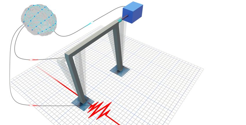
The concept of the intelligent control of the frame is schematically shown in Figure 2. As it is shown, a moment frame
is subjected to the earthquake excitation and the control system transforms the control signals from the neural network
to the horizontal forces on the frame using an actuator. The mass of the frame is 2000 kg, which is considered as a
condense mass at the roof level, the stiffness is 7.9 × 10⁶ [N/s], and the damping is 250 × 103 N.S/m. The natural
frequency ω, and the period T of the system are as follows:
r r
k 7.9e6 1
ω= = = 62.84 (7)
m 2000 s
2π
T = = 0.1 s (8)
ω
7A PREPRINT - JANUARY 27, 2021
Figure 2: Schematic presentation of the structural control problem
5.3 Environment dynamics
The Equation of the motion for the moment frame under the earthquake excitation and the control forces is as follow:
mü + cu̇ + ku = −mẍg + f (9)
in which m, c, k are the mass, damping and the stiffness matrices, ẍg is the ground acceleration, and f is the control
force. u, u̇, and ü are displacement, velocity, and acceleration vectors respectively.
By defining the state vector x as:
T
x = {u, u̇} (10)
The state-space representation of the system would be:
ẋ = Ax + F f + Gẍg (11)
ym = Cm x (12)
Considering v = {ẍg , f }, Equation 11 can be written as:
ẋ = Ax + Bv (13)
in which:
0 1 0 1
A = k c =
−m −m −3947.8 −125.66
0 0 0 0
B = =
−1 1
m
−1 5 × 10⁻⁴
1 0
Cm =
0 1
8A PREPRINT - JANUARY 27, 2021
5.4 Earthquake excitation
In order to train the intelligent controller, the acceleration record of Landers earthquake is considered which is obtained
from the NGA strong motion database [1] (See Figure 3).
8
6
4
Acceleration (m/s 2)
2
0
-2
-4
-6
-8
0 10 20 30 40 50 60
Time (s)
Figure 3: Landers earthquake record, obtained from Pacific Earthquake Engineering Research (PEER) Center [1]
5.5 State
The state shall include all the required data for determining the actions to be an Markov state. In this regard, for
the structural control problem, the ground accelerations as well as the structural responses including acceleration,
velocity, and displacement responses are included in the each state St . Based on the author’s experience, including the
displacements in the last three time steps helps the agent to understand the direction of the motion which is important
specially when reaching the maximums in the oscillations.
{ut , ut−1 , ut−2 , vt , at , üg,t } St (14)
where:
ut : displacement in time t
vt : velocity in time t
at : acceleration in time t
üg,t : ground acceleration in time t
5.6 Reward Function
In reinforcement learning, the reward function determines the goodness of the taken action. In this regard, a multi-
objective reward function is defined including four partial rewards:
Displacement response
The first partial reward function reflects the performance of the controller in terms of reducing the displacement
responses:
| ut |
R1,t = 1 −
umax
in which, ut is the displacement value of the frame at time t and umax is the maximum uncontrolled displacement
response.
Velocity response
This partial reward evaluates the velocity response of the frame:
9A PREPRINT - JANUARY 27, 2021
| vt |
R2,t = 1 −
vmax
in which vt is the velocity response of the frame at time t and vmax is the maximum uncontrolled velocity response.
Acceleration response
The performance of the controller in term of reducing the acceleration responses of the frame is evaluated by R3,t :
| at |
R3,t = 1 −
amax
in which at is the acceleration response of the frame at time t and amax is the maximum uncontrolled acceleration
response.
Actuator force
The goal of the fourth partial reward is to evaluate the required energy by applying a penalty value equal to 0.005 to the
actuator force in each time-step:
R4,t = ft × Pa
in which:
ft = Actuation force at time t (N )
Pa =Penalty value for unit actuator force (= 0.005)
By combining the four partial rewards, the reward value R, at time t will be calculated:
Rt = R1,t + R2,t + R3,t + R4,t
6 Training
Following the experience-replay method, in each training episode, many experiences were recorded in the experience-
replay memory buffer. The algorithm then randomly selected 100 of the records from the experience replay buffer and
experiences were selected by the key state selector function as proposed in [42] to train the Q-net. The target network
was updated every 50 training episodes. The learning parameters have been tuned during preliminary experiments and
are shown in Table 2.
For balancing the exploration and exploitation during the learning phase, the agent followed the -greedy policy which
means that in each state, it took the action with the maximum expected return, but occasionally it took random actions
with a probability of . In this research, a decreasing -value technique is utilized so that its value gradually reduces
from 1 in the beginning to a minimum value of 0.1.
Table 2: Utilized Learning parameters
Number of Size of Number of states Sensor sampling Mini-batch size
episodes experience buffer per episode rate (Hz)
1000 60000 6000 100 50
7 Results
During the learning phase, the controller was trained for three scenarios including zero delay (∆td = 0 s), medium
delay (∆td = 5 s), and long delay (∆td = 10 s). In each scenario, the original and the enhanced methods were utilized
and the maximum-achieved performance of the controller was recorded as presented in Tables 3 to 5. The corresponding
uncontrolled and controlled displacement responses of the frame are demonstrated in Figure 5. The results show that
the enhanced method has significantly improved the performance in all scenarios. Even without action-effect delays, the
performance of the enhanced method in terms of reducing the displacement responses is 46.1% which is much better
than the original method that minimizes the displacement with 7.1%.
10A PREPRINT - JANUARY 27, 2021
Table 3: Seismic responses of the fame in case of zero delay. (Dis. = Displacement (cm), Vel. = Velocity (m/s), Acc.
= Acceleration (m/s2 )).
Learning
Uncontrol. Controlled Improvement
method
Peak Dis. 4.39 4.06 7.1%
Original
Peak Vel. 0.91 0.83 8.7%
method
Peak Acc. 22.97 16.84 26.7%
Peak Dis. 4.39 2.36 46.1%
Enhanced
Peak Vel. 0.91 0.54 41.0%
method
Peak Acc. 22.97 14.28 37.8%
Table 4: Seismic responses of the fame when the delay is 5 seconds (Dis. = Displacement (cm), Vel. = Velocity (m/s),
Acc. = Acceleration (m/s2 )).
Learning
Uncontrol. Controlled Improvement
method
Peak Dis. 4.39 4.24 3.4%
Original
Peak Vel. 0.91 0.85 6.5%
method
Peak Acc. 22.93 20.0 12.8%
Peak Dis. 4.39 3.06 30.2%
Enhanced
Peak Vel. 0.91 0.62 32.2%
method
Peak Acc. 22.93 16.38 28.5%
As it was expected, by increasing the action-effect delay from zero to 5 seconds, the performance of both methods is
reduced, but still the enhanced method, that was utilizing the γ - function for estimating the Q-values, shows a better
performance. For example, in case of having 5 seconds action-effect delays, the performance of the enhanced method
in terms of reducing the displacement responses is 30.2% which is by far better than the value for the original method
with 3.4%.
By studying the performance of both methods under a long action-effect delay (10 seconds), it is understood that the
enhanced method not only significantly improves the performance of the training algorithm but also shows a higher
stability in training an agent for different action-delays. For example, by increasing the delays from 5 seconds to 10
seconds, the performance of the original method in terms of improving the displacement response is dropped from 3.4%
to 0.41%, which implies 87% performance reduction, while the performance of the enhanced method is reduced from
30.2% to 28.2% which indicates only 7% reduction in performance.
In order to better study the performance of both algorithms in case of experiencing long action-effects delays, the
average reward values over the training episodes are presented in Figure 4. As it is shown, the agent achieves a much
better performance within less training episodes when it uses the enhanced method for learning the Q-values.
Table 5: Seismic responses of the fame when the delay is 10 seconds (Dis. = Displacement (cm), Vel. = Velocity
(m/s), Acc. = Acceleration (m/s2 )).
Learning
Uncontrol. Controlled Improvement
method
Peak Dis. 4.39 4.37 0.41%
Original
Peak Vel. 0.91 0.89 1.81%
method
Peak Acc. 22.93 22.31 2.70%
Peak Dis. 4.39 3.15 28.2%
Enhanced
Peak Vel. 0.91 0.66 26.9%
method
Peak Acc. 22.93 17.65 23.0%
11A PREPRINT - JANUARY 27, 2021
2.9 3
2.8
2.8
2.7
2.6
Average reward
Average reward
2.6
2.4
2.5
2.2
2.4
2
2.3
2.2 1.8
0 500 1000 1500 2000 2500 0 500 1000 1500 2000 2500
Training epochs Training epochs
(a) Original method (b) Enhanced method
Figure 4: Average reward during the training episodes in the experiment with 10s delay
8 Conclusions
An enhanced Q-learning method is proposed in which the agent creates a γ - function based on the environment’s
response to a single action at the beginning of the learning phase, and uses that to update the Q-values in each state.
The experimental results showed that the enhanced algorithm significantly improved the performance and stability of
the learning algorithm in dealing with action-effect delays.
Considering the obtained results, the following conclusions are drawn:
1. The enhanced method has significantly improved the performance of the original method in all scenarios with
different action-effect delays. Even without having any action-effect delays.
2. Increasing such delays results in a drop in the performance of the original method while the enhanced method
has shown a stable performance with a small decrease in its performance.
3. It should be mentioned that in the developed method, the γ - function remains constant during the training
phase, which implies that the enhanced method is appropriate for environments with a static behavioral
response to the agent’s actions.
In future work, it would be interesting to study the performance of the enhanced RL algorithm in more complex
simulations using larger structures. We would also like to use the finite response reward filter for other problems in
which there are delays in the effects of actions.
12A PREPRINT - JANUARY 27, 2021
0.05 0.05
Uncontrolled Uncontrolled
0.04 0.04 Controlled
Controlled
0.03 0.03
0.02 0.02
Displacement (m)
0.01 0.01
0 0
-0.01 -0.01
-0.02 -0.02
-0.03 -0.03
-0.04 -0.04
-0.05 -0.05
0 10 20 30 40 50 60 0 10 20 30 40 50 60
Time (s)
(a) Original method - 0 s delay (b) Enhanced method - 0 s delay
0.05 0.05
Uncontrolled Uncontrolled
0.04 Controlled 0.04 Controlled
0.03 0.03
0.02 0.02
0.01 0.01
0 0
-0.01 -0.01
-0.02 -0.02
-0.03 -0.03
-0.04 -0.04
-0.05 -0.05
0 10 20 30 40 50 60 0 10 20 30 40 50 60
(c) Original method - 5 s delay (d) Enhanced method - 5 s delay
0.05 0.05
Uncontrolled Uncontrolled
0.04 Controlled 0.04 Controlled
0.03 0.03
0.02 0.02
0.01 0.01
0 0
-0.01 -0.01
-0.02 -0.02
-0.03 -0.03
-0.04 -0.04
-0.05 -0.05
0 10 20 30 40 50 60 0 10 20 30 40 50 60
(e) Original method - 10 s delay (f) Enhanced method - 10 s delay
Figure 5: Uncontrolled/controlled roof displacement response of the frame when the controller was trained using the
original method and enhanced method.
References
[1] PEER Ground Motion Database - PEER Center. https://ngawest2.berkeley.edu/.
[2] Jürgen Ackermann. Robuste Regelung: Analyse Und Entwurf von Linearen Regelungssystemen Mit Unsicheren
Physikalischen Parametern. Springer-Verlag, 2013.
[3] H. Adeli and A. Saleh. Optimal control of adaptive/smart bridge structures. Journal of Structural Engineering,
123(2):218–226, 1997.
13A PREPRINT - JANUARY 27, 2021
[4] A. S. Ahlawat and A. Ramaswamy. Multiobjective optimal structural vibration control using fuzzy logic control
system. Journal of Structural Engineering, 127(11):1330–1337, 2001.
[5] A. S. Ahlawat and A. Ramaswamy. Multiobjective optimal absorber system for torsionally coupled seismically
excited structures. Engineering Structures, 25(7):941–950, 2003.
[6] A. S. Ahlawat and A. Ramaswamy. Multiobjective optimal fuzzy logic controller driven active and hybrid control
systems for seismically excited nonlinear buildings. Journal of engineering mechanics, 130(4):416–423, 2004.
[7] Mohammad Aslani, Stefan Seipel, Mesgari Mohammad Saadi, and Marco A. Wiering. Traffic signal optimization
through discrete and continuous reinforcement learning with robustness analysis in downtown tehran. Advanced
Engineering Informatics, 38:639–655, 2018.
[8] C. Oktay Azeloglu, Ahmet Sagirli, and Ayse Edincliler. Vibration mitigation of nonlinear crane system against
earthquake excitations with the self-tuning fuzzy logic PID controller. Nonlinear Dynamics, 84(4):1915–1928,
June 2016.
[9] Mark J. Balas. Direct velocity feedback control of large space structures. Journal of Guidance, Control, and
Dynamics, 2(3):252–253, 1979.
[10] Khaldoon Bani-Hani and Jamshid Ghaboussi. Neural networks for structural control of a benchmark problem,
active tendon system. Earthquake Engineering & Structural Dynamics, 27(11):1225–1245, November 1998.
[11] Bani-Hani Khaldoon and Ghaboussi Jamshid. Nonlinear Structural Control Using Neural Networks. Journal of
Engineering Mechanics, 124(3):319–327, March 1998.
[12] Richard Bellman. Dynamic Programming. Princeton University Press, 1957.
[13] Jeremie Cabessa and Hava T Siegelmann. The super-Turing computational power of plastic recurrent neural
networks. International journal of neural systems, 24(08):1450029, 2014.
[14] J. Geoffrey Chase, Scott E. Breneman, and H. Allison Smith. Robust H∞ static output feedback control with
actuator saturation. Journal of Engineering Mechanics, 125(2):225–233, 1999.
[15] Jixiang Cheng, Gexiang Zhang, Fabio Caraffini, and Ferrante Neri. Multicriteria adaptive differential evolution
for global numerical optimization. Integrated Computer-Aided Engineering, 22(2):103–107, 2015.
[16] Hongzhe Dai, Hao Zhang, and Wei Wang. A multiwavelet neural network-based response surface method for
structural reliability analysis. Computer-Aided Civil and Infrastructure Engineering, 30(2):151–162, 2015.
[17] S. N. Deshmukh and N. K. Chandiramani. LQR Control of Wind Excited Benchmark Building Using Variable
Stiffness Tuned Mass Damper. Shock and Vibration, 2014:1–12, 2014.
[18] Francesco Donnarumma, Roberto Prevete, Fabian Chersi, and Giovanni Pezzulo. A programmer–interpreter neural
network architecture for prefrontal cognitive control. International journal of neural systems, 25(06):1550017,
2015.
[19] Richard C. Dorf and Robert H. Bishop. Modern Control Systems. Prentice-Hall, Inc., Upper Saddle River, NJ,
USA, 9th edition, 2000.
[20] John C. Doyle, Keith Glover, Pramod P. Khargonekar, and Bruce A. Francis. State-space solutions to standard
H/sub 2/and H/sub infinity/control problems. IEEE Transactions on Automatic control, 34(8):831–847, 1989.
[21] Gene F. Franklin, J. David Powell, Abbas Emami-Naeini, and J. David Powell. Feedback Control of Dynamic
Systems, volume 3. Addison-Wesley Reading, MA, 1994.
[22] Jamshid Ghaboussi and Abdolreza Joghataie. Active control of structures using neural networks. Journal of
Engineering Mechanics, 1995.
[23] Yoshiki Ikeda, Katsuyasu Sasaki, Mitsuo Sakamoto, and Takuji Kobori. Active mass driver system as the first
application of active structural control. Earthquake Engineering & Structural Dynamics, 30(11):1575–1595.
[24] Mo Jamshidi and Ali Zilouchian. Intelligent Control Systems Using Soft Computing Methodologies. CRC press,
2001.
[25] Jyh-Shing Roger Jang, Chuen-Tsai Sun, and Eiji Mizutani. Neuro-fuzzy and soft computing-a computational ap-
proach to learning and machine intelligence [Book Review]. IEEE Transactions on automatic control, 42(10):1482–
1484, 1997.
[26] Jagatheesan Kaliannan, Anand Baskaran, Nilanjan Dey, and Amira S. Ashour. Ant colony optimization algorithm
based PID controller for LFC of single area power system with non-linearity and boiler dynamics. World J. Model.
Simul, 12(1):3–14, 2016.
14A PREPRINT - JANUARY 27, 2021
[27] Hyun-Su Kim and Paul N Roschke. Design of fuzzy logic controller for smart base isolation system using genetic
algorithm. Engineering Structures, 28(1):84–96, 2006.
[28] Jens Kober, J Andrew Bagnell, and Jan Peters. Reinforcement learning in robotics: A survey. The International
Journal of Robotics Research, page 0278364913495721, 2013.
[29] Arne Koerber and Rudibert King. Combined feedback–feedforward control of wind turbines using state-
constrained model predictive control. IEEE Transactions on Control Systems Technology, 21(4):1117–1128,
2013.
[30] Huibert Kwakernaak and Raphael Sivan. Linear Optimal Control Systems, volume 1. Wiley-interscience New
York, 1972.
[31] William S. Levine. Control System Fundamentals. CRC press, 2019.
[32] Long-Ji Lin. Reinforcement learning for robots using neural networks. PhD thesis, 1993.
[33] Alok Madan. Vibration control of building structures using self-organizing and self-learning neural networks.
Journal of sound and vibration, 287(4):759–784, 2005.
[34] María del Mar Martínez Ballesteros. Evolutionary algorithms to discover quantitative association rules. 2011.
[35] Gang Mei, Ahsan Kareem, and Jeffrey C. Kantor. Model predictive control of structures under earthquakes using
acceleration feedback. Journal of engineering Mechanics, 128(5):574–585, 2002.
[36] Pablo Mesejo, Oscar Ibánez, Enrique Fernández-Blanco, Francisco Cedrón, Alejandro Pazos, and Ana B Porto-
Pazos. Artificial neuron–glia networks learning approach based on cooperative coevolution. International journal
of neural systems, 25(04):1550012, 2015.
[37] Volodymyr Mnih, Koray Kavukcuoglu, David Silver, Andrei A. Rusu, Joel Veness, Marc G. Bellemare, Alex
Graves, Martin Riedmiller, Andreas K. Fidjeland, Georg Ostrovski, Stig Petersen, Charles Beattie, Amir Sadik,
Ioannis Antonoglou, Helen King, Dharshan Kumaran, Daan Wierstra, Shane Legg, and Demis Hassabis. Human-
level control through deep reinforcement learning. Nature, 518(7540):529–533, February 2015.
[38] Moon Seok J., Bergman Lawrence A., and Voulgaris Petros G. Sliding Mode Control of Cable-Stayed Bridge
Subjected to Seismic Excitation. Journal of Engineering Mechanics, 129(1):71–78, January 2003.
[39] Andrew Y. Ng, Adam Coates, Mark Diel, Varun Ganapathi, Jamie Schulte, Ben Tse, Eric Berger, and Eric
Liang. Autonomous Inverted Helicopter Flight via Reinforcement Learning. In Marcelo H. Ang and Oussama
Khatib, editors, Experimental Robotics IX, Springer Tracts in Advanced Robotics, pages 363–372. Springer Berlin
Heidelberg, 2006.
[40] Alexander S. Poznyak, Edgar N. Sanchez, and Wen Yu. Differential Neural Networks for Robust Nonlinear
Control: Identification, State Estimation and Trajectory Tracking. World Scientific, 2001.
[41] Pelayo Quirós, Pedro Alonso, Irene Díaz, and Susana Montes. On the use of fuzzy partitions to protect data.
Integrated Computer-Aided Engineering, 21(4):355–366, 2014.
[42] Hamid Radmard Rahmani, Geoffrey Chase, Marco Wiering, and Carsten Könke. A framework for brain learning-
based control of smart structures. Advanced Engineering Informatics, 42:100986, 2019.
[43] Bijan Samali and Mohammed Al-Dawod. Performance of a five-storey benchmark model using an active tuned
mass damper and a fuzzy controller. Engineering Structures, 25(13):1597–1610, 2003.
[44] Mehdi Soleymani and Masoud Khodadadi. Adaptive fuzzy controller for active tuned mass damper of a benchmark
tall building subjected to seismic and wind loads. The Structural Design of Tall and Special Buildings, 23(10):781–
800, 2014.
[45] Eduardo D. Sontag. Mathematical Control Theory: Deterministic Finite Dimensional Systems, volume 6. Springer
Science & Business Media, 2013.
[46] Richard S. Sutton and Andrew G. Barto. Reinforcement Learning: an Introduction. The MIT Press, 1998.
[47] Gerald Tesauro. TD-Gammon, a self-teaching backgammon program, achieves master-level play. Neural
computation, 6(2):215–219, 1994.
[48] Nengmou Wang and Hojjat Adeli. Algorithms for chattering reduction in system control. Journal of the Franklin
Institute, 349(8):2687–2703, 2012.
[49] C.J. Watkins and P. Dayan. Q-learning. Mach.Learn., (8):279–292, 1992.
[50] Marco Wiering and Martijn van Otterlo. Reinforcement Learning: State-of-the-Art. Springer Science & Business
Media, March 2012.
15A PREPRINT - JANUARY 27, 2021
[51] Di You, Carlos Fabian Benitez-Quiroz, and Aleix M Martinez. Multiobjective optimization for model selection in
kernel methods in regression. IEEE transactions on neural networks and learning systems, 25(10):1879–1893,
2014.
16You can also read