Quarkonium dissociation at the Large Hadron Collider - Technische Universit at M unchen Department of Physics
←
→
Page content transcription
If your browser does not render page correctly, please read the page content below
Technische Universität München

              Department of Physics

                     Bachelor’s Thesis

Quarkonium dissociation at the Large Hadron
                 Collider
                     Georg Stockinger

                       August 2013

            Supervisor: Prof. Dr. Nora Brambilla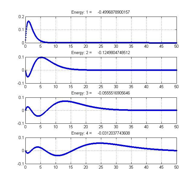
I assure the single handed composition of this bachelor’s thesis only supported by declared
resources.

Munich,
Zusammenfassung
Im Zuge der stehten Entwicklung von Potential Modellen - abgeleitet aus der Quan-
tenchromodynamik - zur Beschreibung der dynamischen Prozesse in einem Quark-Gluon-
Plasma (QGP), werden numerische Methoden zur Lösung komplex wertiger Schrödinger
Gleichungen immer bedeutender. In dieser Arbeit sollen Phänomene, wie sie nur in einem
QGP auftauchen (z.B. ’deconfinement’) vorgestellt werden. Durch das Betrachten des
QGP durch die Augen einer nicht relativistischen effektiven Feld Theorie wird ein Poten-
tial abgeleited, welches eben jene Effekte beschreiben soll. Zur Lösung der so entstandenen
Schrödinger Gleichung werden numerische Methoden zur Hilfe genommen, präsentiert und
getestet.

Abstract
In the course of recent development of potential models - derived from QCD - describing
the dynamics in a quark-gluon plasma (QGP), numerical methods for solving complex
Schrödinger equations become more and more important. In this thesis phenomena which
only appear in the QGP (e.g. ’deconfinement’) shall be described. Seeing the QGP
through the eyes of an non-relativistic effective field theory, a potential incorporating
exactly these attributes is derived. To solve the so found Schrödinger equation auxiliary
numerical methods are presented and tested.
Contents
1 Introduction                                                                                                            1

2 Quark-antiquark potential in a hot medium: real and imaginary part                                                      2
  2.1 EFT approach . . . . . . . . . . . . . . . . . . . . . . . . . . . . . . . . . .                                    2
  2.2 The potential . . . . . . . . . . . . . . . . . . . . . . . . . . . . . . . . . .                                   3

3 Solving the Schrödinger equation                                                                                       4
  3.1 The time-dependent and -independent Schrödinger equation                          .   .   .   .   .   .   .   .    4
  3.2 Finite-differences . . . . . . . . . . . . . . . . . . . . . . . .                 .   .   .   .   .   .   .   .    5
  3.3 Finite-difference time-domain method . . . . . . . . . . . . .                     .   .   .   .   .   .   .   .    7
       3.3.1 Explicit Method . . . . . . . . . . . . . . . . . . . . .                   .   .   .   .   .   .   .   .    8
       3.3.2 Implicit method - Crank-Nicolson . . . . . . . . . . .                      .   .   .   .   .   .   .   .    8
       3.3.3 Finite Difference Matrices - Eigenvalue approach . . .                      .   .   .   .   .   .   .   .    9
  3.4 Calculation of energies . . . . . . . . . . . . . . . . . . . . .                  .   .   .   .   .   .   .   .   11
       3.4.1 Integration and normalization . . . . . . . . . . . . .                     .   .   .   .   .   .   .   .   11
       3.4.2 Calculating higher states by taking snapshots . . . .                       .   .   .   .   .   .   .   .   11
       3.4.3 Fitting the decay . . . . . . . . . . . . . . . . . . . .                   .   .   .   .   .   .   .   .   12

4 Implementation, benchmarks and comparison                                                                              12
  4.1 FDTD - Integration and snapshots . . . . . . .         .   .   .   .   .   .   .   .   .   .   .   .   .   .   .   14
  4.2 FDTD - Fitting the decay . . . . . . . . . . . .       .   .   .   .   .   .   .   .   .   .   .   .   .   .   .   15
  4.3 Finite Difference Matrices . . . . . . . . . . . .     .   .   .   .   .   .   .   .   .   .   .   .   .   .   .   17
  4.4 Summary of numerical methods . . . . . . . . .         .   .   .   .   .   .   .   .   .   .   .   .   .   .   .   18

5 Application to the quark-antiquark potential                                                                           19

6 Conclusions                                                                                                            22

7 Appendix                                                                                                               24
  A  Unit system . . . . . . . . . . .     . . . . . . . . . . . .       .   .   .   .   .   .   .   .   .   .   .   .   24
  B  Coefficients of finite-differences    . . . . . . . . . . . .       .   .   .   .   .   .   .   .   .   .   .   .   24
  C  Simple algorithm for integrating      discrete data arrays          .   .   .   .   .   .   .   .   .   .   .   .   25
  D  Programs and libraries . . . . .      . . . . . . . . . . . .       .   .   .   .   .   .   .   .   .   .   .   .   25
  E  PC Configuration . . . . . . . .      . . . . . . . . . . . .       .   .   .   .   .   .   .   .   .   .   .   .   26

References                                                                                                               27
1
1 Introduction
The quark-gluon plasma (QGP) is a new state of matter predicted by Quantumchromody-
namics (QCD) to form at extremely high temperatures of about 180 MeV. Understanding
the inner behavior of a QGP is of high interest since it was one of the dominant states
of matter in the first fractions of a second of the universe, called the quark epoch. The
fundamental interactions had taken their present forms but the existence of individual
hadrons was not imaginably due to the high temperature and many research groups are
taking up the task of examining this new kind of matter [1, 2, 3, 4]. An introduction to
this topic can be found in [5, 6] including a historical review of the QGP.
Major experiments are now running to examine the quark-gluon plasma. The largest
and most commonly known is the Large Hadron Collider (LHC) at CERN situated near
Meyrin in Switzerland which will eventually collide heavy ions with a maximum energy
of up to 5.5 TeV per nucleon, higher than any other particle accelerator before. At these
1/4
high energies one expects a temperature at collision point of about 830MeV (if T ∼ Ecol )
[3] , more than four times the critical temperature in which the QGP should form.
Experiments at LHC have shown heavy quarkonium suppression, which was proposed as
a signal of deconfinement, a property of a phase in which the quarks in a QGP are free
to move over distances way larger than in their normal hadronic confined phase. Many
proposals have been made to explain this phenomenon of quarkonium suppression. In the
work of Matsui and Satz [7] it is suggested that color screening induced by the thermal
bath leads to a dissociation of quarkonium bound states. Assuming that increasing tem-
perature yields a higher density of gluons (yielding gluo-dissociation) and partons (leading
to dissociation by inelastic parton scattering), quarkonia are scattered by these and disso-
ciate leading to a suppression of quark-antiquark bound states. The often quoted Landau
damping [8] can be related to inelastic parton scattering [9] and the thermal singlet to
octet transition to gluo-dissociation [10], where both are dominant in different energy
scales.
Theoretical endeavors now focus on deriving effective field theories (EFT’s) describing the
behavior of quarkonium bound states depending on the temperature in the QGP. Since
quarkonia like bb or cc are dominated by short distance physics at low temperature, have
binding energies smaller than the quark mass mQ
ΛQCD , sizes much larger than 1/mQ
and satisfy v
c, they provide an excellent probe for the QGP. Utilizing these advantages
a hierarchy of EFT’s in a low energy range can be deduced of which one of them can be
seen as a finite-temperature version of non-relativistic QCD (pNRQCD) [11, 12]. This
effective theory describes the behavior of quarkonium bound states through the view
of potential models. Implying color screening, Landau damping and other contributions
coming from the medium, static potentials characterizing quarkonia at finite temperatures
become complex valued and hence a thermal width of the bound state is induced [13].
This thesis will give an introduction on how the above mentioned potentials can be derived
and then concentrate on solving the three dimensional Schrödinger equation with a com-
plex potential by finite-difference methods. An explicit method [14], an implicit method
and one eigenvalue method is used to obtain numerical results of the bound states. In the
following section the complex quark-antiquark potential is described in all its parts. The
sections thereupon will focus on finite-difference methods used to solve the Schrödinger
equation and are tested on the well known hydrogen atom. After evaluating the efficiency22 QUARK-ANTIQUARK POTENTIAL IN A HOT MEDIUM: REAL AND IMAGINARY PART
of every method solutions of the quarkonium bound states are sought and presented. Ev-
ery part of code and more informations about the numerical methods or formulas used
can be found in the appendix. At last this thesis wants to give a small outlook for future
work.
2 Quark-antiquark potential in a hot medium: real
and imaginary part
2.1 EFT approach
Before focusing on the potential itself it is valuable to have a look on the general aspects
of an EFT characterizing heavy quarkonia. Experimental efforts show that binding en-
ergies of QQ pairs are smaller than their mass m suggesting that all other scales are of
that particular size. Consecutively the velocity v is believed to be much smaller than
c justifying the non-relativistic approach [11]. All this produces a hierarchy of scales
m
mv
mv 2 , namely hard, soft and ultrasoft scale. The idea behind effective field
theories is to ’integrate out’ degrees of freedom not contributing to a certain high range
of energy scale. Effects of these degrees of freedom on lower energy physics are incorpo-
rated in parameters of the EFT. This approach can be made clear when looking at a well
known case like the hydrogen atom 4. Binding energies, the mass of the electron and the
mass of the proton are set in different energy scales making this specific problem easy to
handle. To construct an EFT (e.g. from a more ’fundamental’ Lagrangian of a Quantum
Field Theory (QFT)LQF T or a different EFT) one first identifies these scales matching
the given problem and puts them into a hierarchy. While taking symmetries into account,
one assigns relative weighs (’power counting’) to the terms in the most general EFT that
can be extracted fitting these symmetries. Then, after choosing the required accuracy,
the aforementioned parameters are matched to the ’fundamental’ QFT.
In the context of heavy quarkonium in a hot medium one can utilize non-relativistic and
thermal energy scales. Distinctive energy scales of a non-relativistic QQ bound states are
the mass m, the momentum transfer mv and binding energy mv 2 . Being in a weak coupled
plasma, the temperature T and the Debye screening mass mD ∼ gT are the characteristic
thermal energy scales, where g is the gauge coupling parameter. The EFT describing QQ
pairs with momentum of order mv and energy of order mv 2 is called pNRQCD where
energies above E ∼ mv 2 are integrated out. The Lagrangian LpN RQCD at weak coupling
can be found in [15] and the Hamiltonian in the center-of-mass frame reads
(1) (2)
p2 (0) Vs,o Vs,o
Ĥ = + Vs,o + + 2 + ..., (2.1.1)
m m m
where p = −i∇r . The indices s, o shall differentiate between singlet and octet potentials.
Here higher order terms in the 1/m expansion are neglected . The First term in (2.1.1)
represents the kinetic energy while the second term represents the static potential. For
more detailed information about EFT’s, QCD and especially pNRQCD the reader is
referred to [16, 11, 17, 18].2.2 The potential 3 2.2 The potential In [15] the dissociation of quarkonia due to gluo-dissociation and inelastic parton scat- tering is investigated. Different cross sections of gluons and light quarks in various energy scales are examined and this thesis will concentrate on numerically testing the T mv mD case1 . Remembering that there is a hierarchy of scales the power-counting of in pNRQCD implies that the momentum p and the inverse distance 1/r are approx- imately of the same size. Further the center-of-mass momentum P, the time-derivative and gluon fields scale like energies in a lower range. Consecutively the dominant term in the singlet potentials (2.1.1) is a coulomb like potential [9], which may be only valid for a quarkonium |1si state2 (Υ(1s), J/ψ) in the temperature regime considered.
4                                              3 SOLVING THE SCHRÖDINGER EQUATION

3         Solving the Schrödinger equation
Since finding an analytic solution of the Schrödinger equation is not always possible for
all potentials, one has to use numerical methods to approximate the wave functions and
corresponding energy levels. In order to calculate bound states of quarkonia in a hot
medium, different types of finite-difference methods will be discussed and compared in
the following sections4 .

3.1         The time-dependent and -independent Schrödinger equa-
            tion
For this thesis’ purpose it is necessary to solve the time independent Schrödinger equation
with a static potential V (r, t) = V (r) and a particle of mass m,

                                            En ψn (r) = Ĥψn (r)                            (3.1.1)

where ψn is a quantum-mechanical state, En is the corresponding eigen energy and Ĥ =
−∇2 ~2 /2m + V (r) the Hamiltonian operator.
So the time-independent equation reads

                        En ψn (r) = −∇2 ~2 /2m + V (r) ψn (r)

                                                                               (3.1.2)

For finite-difference time-domain methods it is useful to consider the time-dependent
Schrödinger equation

                              ∂
                                 Ψ(r, t) = ĤΨ(r) = −∇2 ~2 /2m + V (r) Ψ(r, t)

                         i~                                                                 (3.1.3)
                              ∂t
In the case that the potential is spherical symmetric V (r) = V (r) it is possible to simplify
(3.1.2) similar to the classical central-force problem. Consider the Hamiltonian

                                          ~2
                                           H=−
                                             ∆ + V (r).                             (3.1.4)
                                          2m
Finding a solution to (3.1.6) one can use the fact that the angular-momentum operators
l2op and lz commute with H [22], so one can write the solution ψ as eigenfunctions to these
operators

                                                   ul (r)
                                             ψ(r) =       Ylm ,                        (3.1.5)
                                                     r
where Ylm       are the spherical harmonics and ul obeys the radial equation derived in [22]
                           2 2
                                       ~2 l(l + 1)

                              ~ d
                           −         +             + V (r) − En ul (r) = 0.            (3.1.6)
                             2µ dr2       2µr2
Here the reduced mass µ = m1 m2 /(m1 + m2 ) is introduced. Finding a solution to the
above equation leads to a solution to ψ(r).
    4
        For more numerical methods and comparisons the reader is referred to [19, 20, 21]
3.2 Finite-differences 5
3.2 Finite-differences
In order to solve the Schrödinger equation numerically one has to find a way to dis-
cretize and approximate the equation and the solution. One possibility lies in using
finite-differences which are a commonly used since the late 1920’s.
Suppose one has an equally spaced grid with N nodes (x1 , x2 , . . .) on which lies a function
u(xi ).
Figure 1: Grid with N nodes
With the finite difference scheme one tries to approximate the derivation of u(xi ) by
u(xi+1 ) − u(xi )
u0 (xi ) = Forward Difference
h
u(xi−1 ) − u(xi )
u0 (xi ) = Backward Difference
h
1
0 2
u(xi−1 ) + 21 u(xi+1 )
u (xi ) = Central Difference
h
where h is the grid spacing.
To improve accuracy of the numerical derivative one can decrease the value of h or try to
incorporate more grid points, which is accomplished by using undetermined coefficients.
Suppose the pth order derivative of u(xi ) is given by
ai u(xi ) + ai+1 u(xi+1 ) + ....
up (xi ) = + Error.
hp
From here one can, for example calculate, a 2nd order approximation of the first derivative
with the help of the Taylor Expansion,
∞
f 0 (a) f 00 (a) f (n) (a) X f (n) (a)
Pf (x) = f (a) + (x − a) + (x − a)2 + ... + (x − a)n = (x − a)n .
1! 2! n! n=0
n!
The 2nd order approximation of the first derivative reads in general
a1 u(xi ) + a2 u(xi+1 ) + a3 u(xi+2 )
u0 (xi ) = + Error. (3.2.7)
h
and Taylor expansions about xi are
u(xi ) = u(xi )
h2 00 h3
u(xi+1 ) = u(xi ) + hu0 (xi ) + u (xi ) + u000 (xi ) + O(h)4
2 66 3 SOLVING THE SCHRÖDINGER EQUATION
4h3 000
u(xi+2 ) = u(xi ) + 2hu0 (xi ) + 2h2 u00 (xi ) +
u (xi ) + O(h)4 .
3
Substituting this into (3.2.7) and rearranging yields the following linear system:
I (a1 + a2 + a3 )/h = 0
II (a2 + 2a3 ) = 1
III (a2 /2 + 2a3 )h = 0
Solving this system leads to the 2nd order approximation:
−3u(xi ) + 4u(xi+1 ) − u(xi+2 )
u0 (xi ) = + Error. (3.2.8)
2h
The error in the above equation can be deduced again with the Taylor series to
1
Error = h2 u000 i . (3.2.9)
3
This procedure amounts to an improvement of accuracy for finite-differences. A table of
the coefficients of some orders and higher derivatives5 is given in the appendix (B).
With the discretization of the second derivative of 1st order accuracy one can approximate
the Schrödinger equation by replacing the ’real’ derivatives by their finite-differences.6
Consecutively the time derivative in (3.1.3) becomes
∂ Ψ(r, t + ∆t) − Ψ(r, t)
Ψ(r, t) ≈ (3.2.10)
∂t ∆t
where ∆t is a small increment in time.
Using finite-differences on the spatial derivative in 3 dimensions and incorporating the
potential leads to
1
[Ψ(x + ∆x, y, z, t) − 2Ψ(x, y, z, t)] + Ψ(x − ∆x, y, z, t)] (3.2.11)
2∆x2
1
+ [Ψ(x, y + ∆y, z, t) − 2Ψ(x, y, z, t)] + Ψ(x, y − ∆y, z, t)]
2∆y 2
1
+ [Ψ(x, y, z + ∆z, t) − 2Ψ(x, y, z, t)] + Ψ(x, y, z − ∆z, t)]
2∆z 2
1
− V (x, y, z)[Ψ(x, y, z, t) + Ψ(x, y, z, t + ∆t],
2
5
For this thesis purpose it is sufficient to concentrate on the second derivative of 1st order accuracy,
since this reduces computation time and makes the implementation more efficient.
6
From here on atomic units are used if not otherwise mentioned. The reader is referred to the appendix
for further details.3.3 Finite-difference time-domain method 7
which is a discretization of the right side of (3.1.2).
In the last term the wave function is averaged in time. This is done to stabilize the
algorithm [14]. If the potential has a singularity, one has to make sure that none of the
lattice points coincides with it.7
3.3 Finite-difference time-domain method
The finite-difference time-domain method (FDTD) has a long history in computational
physics. It was mainly used in electrodynamics due to its simple form but can be used
for solving the Schrödinger equation as well.
In the FDTD one approximates time and spatial derivatives by their finite-differences. A
solution of a partial differential equation (PDE) is then gained through evolving an initial
function in time. This can be done either by an explicit or an implicit method. Explicit
methods rearrange the discretized PDE that an update equation can be build. A point
in space in the next time step is directly calculated through a formula incorporating the
coordinates of the time step before. An implicit method achieves this evolution by solving
a linear system. Here not one point is extracted from the time step behind, but the full
function is gained by solving this system of equations.
To use this method -regardless of choosing the explicit or implicit way- in quantum me-
chanics one can expand the solution of (3.1.3) in terms of basic functions of the time-
independent problem,
∞
X
Ψ(r, t) = an ψn e−iEn t , (3.3.12)
n=0
where an are expansion coefficients which are fixed by initial conditions and En is the
eigenenergy to a certain state. The index n represents a full set of quantum numbers.
In a one dimensional case n=0,1,2... and is corresponding to the ground state, the first
excited state etc.
If one assumes no singularities exist one can perform a Wick rotation to imaginary time,
τ = it which leads to
∂ ∇2
Ψ(r, t) = Ψ(r, t) − V (r)Ψ(r, t) (3.3.13)
∂τ 2
This equation has a solution of the form
∞
X
Ψ(r, τ ) = an ψn e−En τ . (3.3.14)
n=0
Since the ground state E0 has the lowest energy and energies increase monotonic with
n, the wave function Ψ(r, τ ) will be dominated by the lowest state a0 ψ0 (r)e−E0 τ . Conse-
quently one obtains
lim Ψ(r, τ ) ≈ a0 ψ0 (r)0 e−E0 τ . (3.3.15)
τ →∞
7
For further information about finite difference methods the reader is referred to [23], [24, 25, 26]8 3 SOLVING THE SCHRÖDINGER EQUATION
3.3.1 Explicit Method
In this section an explicit method to solve the Schrödinger equation is presented. It relies
strongly on [14] and basically the same method is used. Differences will show up when
evaluating the efficiency and accuracy of this method.
To simplify (3.2.11) one can set ∆x = ∆y = ∆z = a and write the finite derivative as a
vector
1
~ = 1 −2
D (3.3.16)
a2
1
as well as represent Ψ as a matrix valued Ψ̂ field
Ψ(x − a, y, z, τ ) Ψ(x, y − a, z, τ ) Ψ(x, y, z − a, τ )
Ψ̂ = Ψ(x, y, z, τ ) Ψ(x, y, z, τ ) Ψ(x, y, z, τ ) . (3.3.17)
Ψ(x + a, y, z, τ ) Ψ(x, y + a, z, τ ) Ψ(x, y, z + a, τ )
Now equation (3.2.11) can be written as follows:
3
1X ~ 1
(D · Ψ̂)i − V (x, y, z)[Ψ(x, y, z, τ ) + Ψ(x, y, z, τ + ∆τ )] (3.3.18)
2 i=1 2
Bringing together equations (3.1.3), (3.3.18) and (3.3.13) leads to an update equation in
imaginary time
3
B∆τ X ~
Ψ(x, y, z, τ + ∆τ ) = AΨ(x, y, z, τ ) + (D · Ψ̂)i , (3.3.19)
2m i=1
where A and B are given by
∆τ
1− 2
V (x, y, z) 1
A= ∆τ
B= ∆τ
(3.3.20)
1+ 2
V (x, y, z) 1+ 2
V(x, y, z)
with reintroduced mass m. With (3.3.19) one can now evolve the solution in time and
get the wave function of the ground and excited states with the methods shown in 3.4
3.3.2 Implicit method - Crank-Nicolson
Seeking an implicit method for solving a partial differential equation (PDE) like the
Schrödinger equation, the Crank-Nicolson method (developed by John Crank and Phyllis
Nicolson) will emerge shortly. It is wide spread solving the heat equation and persuades
through its stability.
One still seeks a solution to (3.3.13) therefore a solution to (3.1.3) in imaginary time. To
build an implicit method one can make the assumption that
1 − 21 Ĥ∆τ
e−Ĥ∆τ ≈ (3.3.21)
1 + 21 Ĥ∆τ
which is the so called Cayley F orm [27]. Rearranging suggests an evolution of the form3.3 Finite-difference time-domain method 9
1 1
(1 + Ĥ∆τ )ψkτ +∆τ = (1 − Ĥ∆τ )ψkt (3.3.22)
2 2
Utilizing the known discretization (3.2.11) yields a linear system
N
X
Aij ψjτ +∆τ = bi i = 0, ...N (3.3.23)
j=0
where Aij and bi are
(
1 + ∆τ 1
2 m∆x2
+ Vi i=j
Aij = ∆τ
− 4m∆x2 i=j±1
l
i=0
∆τ ∆τ ∆τ
τ
bi = ψi−1 + 1− 4m∆x2
− V
2 i
ψiτ + ψτ
4m∆x2 i+1
110 3 SOLVING THE SCHRÖDINGER EQUATION
1 1
m∆a2
+ V1 − 2m∆a2
− 1 2 1
+ V2 − 2m∆a1
2m∆a m∆a2 2
1 1 1
− 2m∆a2 m∆a 2 + V3 − 2m∆a 2
~ ~
ψ = En ψ (3.3.25)
.. .. ..
. . .
which can be solved using standard algorithms in the case that V (r) =3.4 Calculation of energies 11
3.4 Calculation of energies
Since the first two methods evolve (3.3.12) in imaginary time the solution sought decays
exponentially. There are now different ways to calculate the energy and the position
representation of the wave function.
3.4.1 Integration and normalization
One way to calculate the energy of a wave function is to reckon the expectation value of
the Hamiltonian operator divided by the normalization of the wave function
R ∗
hψ0 |Ĥ|ψ0 i ψ Ĥψ0 d3 x
E0 = = R 0 2 3 (3.4.28)
hψ0 |ψ0 i |ψ0 | d x
To ensure that the values of the numerically calculated wave function are not too small
for computation one constantly renormalizes the wave, resulting in a simple algorithm
Figure 3: Flowchart for FDTD
Following this algorithm equations (3.3.19) and (3.3.23) can be solved on a 3D-lattice
with lattice spacing a, time increments ∆τ and N lattice nodes in each direction, while
renormalization of the wave function is carried out at certain points of time. One takes
an arbitrary initial wave function for time development. During time evolution snapshots
are being taken which is of use in calculating the excited states. In order to calculate
the energy of the wave function one uses a discrete version of (3.4.28). A rule to perform
integrals on a discrete grid can be found in the appendix. This calculation is done peri-
odically as well, to check, if the wave function has converged to the ground state. The
loop breaks, if a certain tolerance of energy change is reached.
3.4.2 Calculating higher states by taking snapshots
One possible method used by [14] to compute the energy and wave functions of higher
states is to take snapshots during the time evolution of the wave function.12 4 IMPLEMENTATION, BENCHMARKS AND COMPARISON
Consider a wave function Ψsnap (r, τs ) saved at evolution time τs . This wave function can
be written in terms of (3.3.12) as
∞
X
Ψsnap (r, τs ) = an ψn e−iEn t . (3.4.29)
n=0
For large times only the ground state dominate so one can approximate the above equation
as
lim Ψsnap (r, τs ) ≈ a0 ψ0 (r)e−E0 τ . (3.4.30)
τs →∞
After renormalization one can now remove the contribution from the ground state |ψ0 i
leading to a new wave function
|ψ1 i ≈ |Ψsnap i − |ψ0 ihψ0 |Ψsnap i. (3.4.31)
This new found wave function should now contain only contributions from the excited
states’ wave functions and it follows that for large times
lim |ψ1 i ≈ a1 ψ1 (r)e−E1 τ ,
τs →∞
where ψ1 (r) denotes the first excited state. With the iterative method provided in [31]
one can theoretically compute as much excited states as the amount of wave functions
saved during the evolution. To assure that this method works properly it is important to
set the snapshot time τsnap
1/(E2 − E1 ) [14].
3.4.3 Fitting the decay
Another way of proceeding is to use the fact that -for large imaginary times- the norm of
the wave function decreases exponentially (3.3.15). This suggests that one can record the
~ = a, y = b, z = c) for any a, b, c and fit its behavior by
time evolution of one point ψ(x
fDecay (τ ) = Ae−γτ .
To extrapolate the excited states an additional term is appended to the above equation
fDecay (τ ) = A0 e−E1 τ + A1 e−E2 τ .
This addition can be made several times, but, following from (3.3.15), the dominant state
is still the ground state suppressing the higher states in the fit. This can make it hard to
calculate states above E3 . In addition to that a recovery of the position representation
of the full wave may be impossible due to the advanced time evolution. The numerical
values representing the wave function could be too small to be renormalized.
4 Implementation, benchmarks and comparison
This section will give the reader some information about the implementation8 of the
aforementioned numerical methods as well as about their accuracies. At the end the
8
A full code of all methods is available at https://sourceforge.net/projects/finitediff/files/13
results of each method are matched against each another. To get a notion of the accuracy
and performance of the finite-difference methods one should use a well known case like
the Hydrogen atom with its Hamiltonian (without any corrections like Lamb-shift etc.)
1 1
H=− ∆− (4.0.1)
2m r
in the Hartree unit system (A)9 . Since this Hamiltonian is spherical symmetric one can
utilize (3.1.6) for simplification and then calculate the solutions analytically leading to
n = nr + l + 1 (4.0.2)
1
Enr l = −
2(nr + l + 1)2
s l
2 nr ! 2r 2r r
ψnlm (r) = 2 L2l+1
nr e− n Ylm (θ, φ) = |nlmi
n (n + l)! n n
where L2l+1
nr are the Laguerre polynomials, Ylm (θ, φ) are the spherical harmonics and
nr , l = 0, .., N are the quantum-numbers.
The first eigenvalues and -functions should therefore read
1 1 1
E1 = − , E2 = − , E3 = − ,
2 8 18
ψ100 (r) = 2e−r = |1si
1 1
ψ200 (r) = √ (1 − r)e−r/2 = |2si
2 2
2 2 2
ψ300 (r) = √ (1 − r + r2 )e−r/3 = |3si
3 3 3 27
The FDTD methods are implemented in C++ and the finite-difference matrix method
regards the use of MATLAB. The implicit method is a pure one dimensional code whereas
a one and a three dimensional version similar to [14] of the explicit method is available.
Programming in C++ or any other coding language has the advantage of having direct
control over all functions and the possibility to optimize and debug them if needed. MAT-
LAB provides efficient built in algorithms (e.g. handling of sparse matrices etc.) but one
needs to take special attention to memory allocation since MATLAB itself has to run to
execute script files which occupies additional memory.
With this knowledge one can now put the numerical methods to the proof 10 .
9
It shall be noted that using this unit system simplifies the parameters used in the written code.
Setting the mass parameter to 1, all following numerical evaluations can be reproduced without any
other customization needed
10
All the numerical tests are done on a standard PC running a Linux system. Only MATLAB requires
a Microsoft Windows System. The PC’s configuration can be found in the appendix14 4 IMPLEMENTATION, BENCHMARKS AND COMPARISON
4.1 FDTD - Integration and snapshots
Benchmark
In this section both the explicit and the implicit method are following the procedure
depicted in Fig. (3).
A grid of N = 1000 nodes with a spatial step of ∆a = 0.05 and a time step of ∆τ = 0.001
is used to calculate the wave function using I = 150, 000 iterations. As initial condition
a Delta Peak (ψ(r = N/2) = 1) and a discretized Dirac Delta (−6Nc rδ(r)[2]) is used. In
both cases the energy is calculated via (3.4.28) and amounts to
E1 = −0.499531,
giving an error of 0.0937% for the ground state energy, reckoned by the explicit method.
Using the Crank-Nicolson method results in
E1 = −0.5099,
differing about 2% from the result of the explicit method.
Figure (4) shows the numerically calculated wave function and the analytic radial solution
of the Hydrogen atom u0 (r) = ψ0Y(r)r
00
.
Figure 4: Ground state calculated with the explicit FDTD method
Both implementations took 1.6 minutes to calculate the ground state needing 0.0009602
seconds for one iteration.
The excited states wave functions and energies shall be calculated by taking snapshots
during the time evolution and utilizing (3.4.31). Unfortunately taking a one dimensional
version of the code11 presented in [14] did not yield correct results. Testing the full
11
M. Strickland, Parallelized FDTD Schrödinger Solver, http://sourceforge.net/projects/quantumfdtd/
(2009).4.2 FDTD - Fitting the decay 15
implementation was not possible as well despite having installed and tested the required
Message Passing Interface12 (MPI).
To get to the excited states nonetheless the time evolution is done multiple times. The
first evolution done results in the above calculated ground state Fig. (4). During the
second time evolution the contribution of the ground state is constantly removed from
an arbitrary initial wave function or a snapshot with (3.4.31) leading to an excited state
energy
E2 = −0.1231
and an error of 1.47%. Applying the implicit method resulted in E2 = −0.1262.
This second evolution was done with a total time about twice as large as the time used
for calculating the ground state to ensure convergence. To reach even higher states it is
possible to do a third evolution subtracting the contributions from the ground as well as
from the first excited state and so forth.
Manipulating the angular momentum leads to the following energies Enr ,l ,
E0,1 = −0.1250050 Error = 0.04%
E0,2 = −0.0555479 Error = 0.01%
E0,3 = −0.0312147 Error = 0.11%
which are computed by the explicit method again. These values are quite accurate and
can be interpreted as the |2pi, |3di . . . states of the Hydrogen atom.
4.2 FDTD - Fitting the decay
Benchmark
The implementations are now manipulated in the way that they record the behavior of a
value ψ(r = ∆a, t) during the evolution which is expected to be a decay similar to (3.4.3).
Grid parameter are chosen to be the same as in the section before with a slight change
in the time step ∆τ = 0.0001 to record a sufficient amount of data which is essential for
an accurate fitting procedure. Figure (5) pictures the decay of ψ(r = ∆a, t), produced
with the implicit method, starting from 60% of the iterations (I = 150, 000) until the
end, and the fitting curve. To guarantee that the evolution decays (the parameters En
of (3.4.3) have to be positive), a constant of c = 2 is added to the coulomb potential
which increases the energy of the ground state to E10 = −1/2 + 2 = 1.5 and of the first
excited state E20 = −1/8 + 2 = 1.875. In a general case it is useful to add the mass of
the examined particles 2m to the potential ensuring positive energies and so the resultant
binding energy can be calculated afterwards via
Ebinding = Ecalculated − 2m. (4.2.3)
As one can see the results are not that accurate as the results of the explicit method.
Furthermore the analytical results do not lay within the margin for error calculated by
12
http://www.open-mpi.org/16 4 IMPLEMENTATION, BENCHMARKS AND COMPARISON
Figure 5: Decay of initial wave
GNUPLOT. The computation took again 1.6 minutes but to fit the decay GNUPLOT
needed more than 2 hours. The difficulties arising with this method are that one has to
carefully choose the timespan in which the decay is recorded and which point of the initial
function one should follow. Furthermore it is important to ensure a decay ( limτ →∞ ψ(r =
c, τ ) = 0) by manipulating the potential to give positive results, which otherwise would
lead to increasing errors in increasing time. Speaking of a decay in this context means that
( limτ →∞ A0 ψ(r = c, τ ) = 0) is ensured regardless of the sign of A0 which is predefined by
the representation of the initial condition in the set of basis therms of the sought solution
(3.3.12).4.3 Finite Difference Matrices 17
4.3 Finite Difference Matrices
Benchmark
Program parameters like grid discretization or spatial steps are equal to the parameters
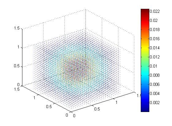
of the explicit method. Running the MATLAB script leads to the results shown in Fig.
(6).
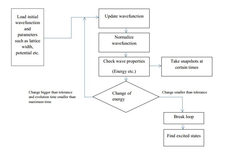
Figure 6: The first four eigenenergies and corresponding radial solutions
The graphs shown represent the |1si, |2si, |3si and |4si state of the radial solution u(r).
Having a closer look at the plots noticeable that the |2nsi (n = 1, 2, 3 . . .) states have the
opposite sign of their analytical results, which may come from the algorithms MATLAB
uses, but this does not affect orthogonality of the results or the probability density |ψ|2 .
Striking about these results however is the small error in all energy states which is 0.15% at
maximum. Especially if one considers that MATLAB took just 1.134 seconds computation
time.
Generalizing the script to three dimensions nevertheless greatly reduces accuracy for mem-
ory reasons. The maximum grid size the PC was able to handle was N = 243 nodes. The
so calculated energy E1 = 9.42624 is conceivable far away from the correct result.. The
explanation to this can be found by having a closer look on the units used for computing.
Taking a grid of N = 243 nodes and a grid spacing of ∆a = 0.05 the length of one edge of
the computation volume is 24 × 0.05 = 1.2ab . Considering that a great part of the radial
solution lays on distances
ab this result can be understood. Producing a 3D plot of18 4 IMPLEMENTATION, BENCHMARKS AND COMPARISON
this state can just show qualitatively the properties of the |1si state.
Figure 7: 3D plot of the |1si state with N = 243 nodes
At least one can still see that the probability of finding the electron close to the hydrogen
atom is bigger than finding it at a certain distance.
4.4 Summary of numerical methods
As conclusion one can say that the direct eigenvalue approach seems to produce the best
and most accurate results. It is fast and straightforward to implement and to understand
but has its disadvantages as well. It is hard to change to boundary conditions which are
now standard Dirichlet boundary conditions meaning that ψ(0) = ψ(∞) = 0 , respectively
ψ(−∞) = ψ(∞) = 0. Absorbing boundaries or any other kind of boundary conditions,
which are easily implemented in the other two methods, are therefore disregarded. Fur-
thermore simulating bigger sized grids is almost impossible when running the script on a
standard home computer.
Using both finite-difference time-domain methods following the steps depicted in (3) leads
to valuable results with only small differences. The first excited state can be calculated
to a good accuracy as well as states with higher angular momentum with both methods.
An advantage of the explicit method is that it is straightforward to implement and main-
tain as well as easily to generalize to three dimensions [14]. The latter however greatly
increases memory and CPU usage so one has to greatly decrease the grid size used in the
sections before, to achieve results in a reasonable timespan, resulting in a loss of accu-
racy. Consecutively one should use the implementation presented in [14] with powerful
computational devices. In comparison to the implicit method though it lacks stability for
some applications. Time stepping and spatial stepping have to be chosen accurately to
ensure bugless performance. During the evaluation of the section before special attention19
was paid to achieve a stable implementation. The Crank-Nicolson method however was
always stable but is somewhat harder to maintain. Special attention is regarded in check-
ing the LU-algorithm and setting the updated vector ~b (3.3.2). Just a generalization to
three dimensions is more complicated in comparison to the explicit method.
Combining these methods with the fitting method results in a decrease of efficiency and
makes the calculation of energies more complicated. The numerically calculated eigenen-
ergies depend on the range of time in which the decay is recorded. It is important to set
the initial parameters of the fitting algorithm to values considerably close to their correct
result. Otherwise the fit does not converge accurately or gives large margin for errors.
Furthermore one has to make sure that the recording is starting at a time large enough,
so that most higher states have no contribution, while simultaneously finding the right
point of time to end the recording, so that values are not to small to fit accurately.
5 Application to the quark-antiquark potential
To simplify the application of the numerical methods ,just presented in the sections before,
a slight change units system is carried out (A). In this thesis the examined quarkonium
shall be bottomonium (bb) assuming the mass of the bottom quark in the new units to be
mbottom = 4.14GeV
The temperatures considered in the numerical estimations are T = 400Mev and T =
250MeV. In addition the dependency of the imaginary part of the potential on the strong
coupling constant shall be revealed by varying its numerical value between 0 . . . 0.41 in
the imaginary part of the potential, while fixing the Bohr radius a0 = 2/(mCf αs ).
As it has been noted in 2.2 the real and imaginary part of the ground state will be
compared with the analytically found solution.
The real part ER can be extracted considering the fact that the real part of the potential
is coulomb like [9]:
mbottom Cf2 αs2
ER = − ≈ −0.3093GeV (5.0.1)
4
For the imaginary part one inserts (2.2) in (2.2.5) resulting in
2 3 4 3
Eimag (αs , T ) ∼ −Γ(αs , T )/2 ∼ −cαs Cf T ln − , (5.0.2)
αs T 2 c 2
N
where c = ( 4π a2 )(Nc + 2f ).
3 0
In the following the aforementioned methods will be applied to the given potential. The
real and the imaginary part of the ground state energy will be calculated for different
temperatures.
Calculations with the fitting method
Staying in the environment already used in 4.2 the FDTD methods record the value of
ψ(r = ∆a, τ ) during the time evolution. After acquiring data over a long time span one
can use the behavior of this value to calculate of the energy of the resultant wave function.20 5 APPLICATION TO THE QUARK-ANTIQUARK POTENTIAL
Since the potential in this case is complex valued and so the energy of the ground state
(E0 = ER + iEI ) as well, one expects for large imaginary times (3.3.15) that
ψ(r = ∆a, τ ) ≈ A0 e−E0 τ = A0 e−ER τ (cos(EI τ ) − i sin(EI τ )), (5.0.3)
hence the decay oscillates with an angular frequency ω = EI . To record the full oscillation
needed for an accurate fit the time span, in which ψ(r = ∆a, τ ) is recorded, should
therefore be τ = EπI . At this point of time the wave function can be estimated
E
− ER π
ψ(r = ∆a, τ ) ≈ A0 e I (5.0.4)
Considering that one has assumed that the imaginary part of the potential is small against
the real part the time span to observe must be very long. In addition this the point of
time to start the record has be chosen large enough to make sure (5.0.3) gives a valid
approximation (3.3.15). At times so large changes in the value of ψ(r = ∆a, τ ) could be
too small to calculate EI .
Using the implicit method to record (5.0.3) a valuable approximation could unfortunately
only be achieved for the real part of the ground state energy for the aforementioned
reasons,
ER = −0.30522GeV,
which is the mean value of several attempts. The grid size was set to N = 2000, the
time and spatial step to ∆τ = 0.01 , ∆a = 0.05. The value of ψ(r = ∆a, τ ) was recorded
during 600,000 iterations starting at 40% of the total time until the end.
Explicit and implicit method
Due to the arguments given in the section before the programs responsible for the cal-
culation are adjusted ensuring that both evolution methods - explicit and implicit - are
running the algorithm depicted in Fig. (3). Grid parameters are chosen to be the same
in each implementation:
N = 2000 ∆τ = 0.0001 I = 500, 000
In Fig. (8) the real part of the computed energy is shown for T = 400MeV, T = 250MeV
and both methods. At high temperatures and high αs the imaginary part of the potential,
in which the temperature is implied, seems to have effect of the real part of the binding
energy. The deviation of the analytical result sums up to 5% when looking at the case T =
400MeV, αs = 0.41. Looking at small αs (Fig. 9) in both methods seemingly reveals the
relation limαs →0 = limEimag (αs )→0 = 0 (computed up to values of αs = 2.658829 × 10⁻¹⁵ ).
In this limit the real part of the energy was reckoned to
ERexplicit = −0.308952GeV Error = 0.1%
ERimplicit = −0.3125GeV Error = 2.3%21
Figure 8: ER for T = 400MeV, 250MeV Figure 9: EI at small αs
As it can be seen in Fig. (9) the numerical values match very good with the analytical
results. The plots below picture the numerical results of the imaginary part coming from
both methods together with the analytical results derived from (5.0.2).
Figure 10: T=250MeV Figure 11: T=400MeV
Following from the graphs shown it can be said that both methods produce similar results
over the whole range of variation of αs . In the case that T = 250MeV analytical and
numerical computations fit perfectly, however when T = 400MeV numerical results start
differing from their analytically computed counterparts at αs ≈ 0.2.22 6 CONCLUSIONS
Finite-difference matrices
Taking the grid parameters from the FDTD methods and applying them on the matrix
method reveals the same behavior shown in Fig. (8) and a value at small αs
ERimp = −0.3089GeV.
This results deviates only 0.1% from the analytical achieved solution.
The dependency of the imaginary part on the temperature and the strong coupling αs is
shown in the figures (12) and (13).
Figure 12: T=250MeV Figure 13: T=400MeV
Fig. (12) shows the numerical achieved results in comparison with the analytical values.
They assort over the whole range of αs . At higher temperatures the findings of the matrix
method deviate from the analytical results if αs > 0.2. Looking at the limit limαs →0 results
in a significant deviation as well for both temperatures. For illustration one could take
the numerical value at αs = 4.1 × 10⁻⁴ computed by the matrix method at T = 400MeV
is EI = −4.698 × 10⁻⁶ . Calculating the analytical result yields EI = −7 × 10⁻⁷ which
is about 1 order of magnitude off the aforementioned value. It seems that in this limit
the matrix method is failing or that -considering the spatial step- accuracy is not high
enough to gain valuable results in this energy or αs range.
6 Conclusions
Comments on the results
The computation done with the FDTD leads to very similar results with more accuracy
in the real part when using the explicit method. They produce the same values sweeping
over the whole range of 0 < αs < 0.41. The same can be said about the matrix method
when comparing FDTD methods with this eigenvalue approach. Especially in the case
T = 250MeV all methods work accurate and efficient. Looking at small values however
the matrix method seems to reach it’s limits. The results presented at a temperature
T = 400MeV match among themselves and until αs ≈ 0.2.23 Opportunities for improvement A chance to improve accuracy and efficiency could lay in implying a more accurate deriva- tive meaning that the discretized derivation takes more points of the grid into account [23]. This can be achieved with the coefficients which have been introduced in section 3.2 especially when using them with an explicit method. Using them with an implicit method one would need fast algorithms to find solutions to non-tridiagonal linear systems. Re- garding the matrix method a possible increase in accuracy as well as in efficiency could lay in using the spectral methods provided in [30] which are tested for complex valued problems as well. Outlook After testing the finite-difference methods on a well known case and a potential coming from recent research there is now the time to contribute to theoretical endeavors focus- ing on the QGP. These methods can be generalized to three dimensions so anisotropic potentials can be put to the test as well, hopefully giving new insights in the physics behind.
24                                                                                                7 APPENDIX

7     Appendix
A     Unit system
Hartree
To simplify notation in the Schrödinger equation of the hydrogen atom it is common to
use the Hartree units in which the following changes are carried out:
                                           ~ = me = e = 4π0 = 1
                                               1
                                           c=
                                               α
               1
where α ∼     137
                    is the fine-structure constant. This yields an energy unit of
                                                 EH ≈ 27.2eV
and a unit of length aB = 1.

QCD
In QCD it is appropriate to use an energy unit which is sufficiently larger than the Hartree
unit. The following adjustments to the SI-units are conducted
                                                       ~=1
                                                       c=1
Following from that physical values can be described in powers of energy, e.g masses now
have the unit E 1 , lengths and time E −1 .

B     Coefficients of finite-differences
                                                  Central Difference
     Derivative   Accuracy     -4      3           2          1         0        1        2         3        4
         1           2                                       1/2        0       1/2
                     4                           1/12        2/3        0       2/3      1/12
                     6                1/60      3/20         3/4        0       3/4      3/20      1/60
         2           2                                        1         2        1
                     4                           1/12        4/3       5/2      4/3      1/12
                     6                1/90      3/20         3/2     49/18      3/2       3/20    1/90
         3           2                           1/2          1         0        1        1/2
                     4                 1/8         1        13/8        0      13/8        1       1/8
                     6       7/240    3/10     169/120     61/30        0      61/30    169/120    3/10     7/240
         4           2                             1          4         6        4         1
                     4                 1/6         2        13/2      28/3     13/2        2       1/6
                     6       7/240      2/5    169/60      122/15     91/8    122/15    169/60     2/5      7/240
                                            Forward/Backward Difference
                                0        1         2          3         4       5         6         7        8
         1           1          1        1
                     2         3/2       2       1/2
                     3        11/6       3        3/2        1/3
         2           1          1        2         1
                     2          2        5         4          1
                     3        35/12   26/3      19/2        14/3      11/12
         3           1          1        3         3          1
                     2         5/2       9        12          7        3/2
                     3        17/4     71/4      59/2       49/2      41/4      7/4
                     6       801/80   349/6   18353/120   2391/10    1457/6   4891/30   561/8     527/30   469/240
         4           1          1        4         6          4         1
                     2          3       14         26        24        11        2
                     3        35/6      31      137/2      242/3      107/2     19       17/6

                              Table 1: Finite-difference coefficients [32]
C Simple algorithm for integrating discrete data arrays 25
C Simple algorithm for integrating discrete data arrays
To calculate the energy or the norm of a wave function one needs to integrate over the
data array in which the wave is stored. A simple way to do this is to use a trapezoidal
rule. To calculate the area one finds
Figure 14: Trapezoidal rule
1
A= (f (xi ) + f (xi+1 )),
2∆x
giving the approximation
Zb b
∆x X
f (x)dx ≈ (f (xi ) + f (xi+1 )).
2 i=a
a
Generalizing to 3 dimensions leads to
Zzb Zyb Zxb xb yb zb
∆a3 X X X
f (x, y, z)dxdydz ≈ (f (xi , yj , zk )+
8 x =x y =y z =z
z a ya xa i a j a k a
f (xi+1 , yj , zk ) + f (xi , yj , zk+1 )+
f (xi+1 , yj+1 , zk ) + f (xi+1 , yj , zk+1 )+
f (xi , yj+1 , zk+1 ) + f (xi+1 , yj+1 , zk+1 )).
D Programs and libraries
In this thesis additional programs aside from the self-implemented ones have been used.
To plot most of the graphs ’QtiPlot’ [33] was used. Fitting the decay regarded the help
of GNUPLOT [34].
The implementation of the self-written programs was partly done with the support of the
GSL-library [35], a C++ numerical library, as well as with MATLAB [29], a computer
algebra system.26 7 APPENDIX
E PC Configuration
Operating System : Linux Ubuntu x64/ Microsoft Windows 8 x64
RAM : 4 GB
Processor : 8 × Intel Core i7 Q720 @ 1.60GHzREFERENCES 27
References
[1] N. Brambilla, S. Eidelman, B.K. Heltsley, R. Vogt, G.T. Bodwin, et al. Heavy
quarkonium: progress, puzzles, and opportunities. Eur.Phys.J., C71:1534, 2011.
[2] M. Laine. A Resummed perturbative estimate for the quarkonium spectral function
in hot QCD. JHEP, 0705:028, 2007.
[3] Matthew Margotta, Kyle McCarty, Christina McGahan, Michael Strickland, and
David Yager-Elorriaga. Quarkonium states in a complex-valued potential. Phys.Rev.,
D83:105019, 2011.
[4] Nora Brambilla, Jacopo Ghiglieri, Antonio Vairo, and Peter Petreczky. Static quark-
antiquark pairs at finite temperature. Phys.Rev., D78:014017, 2008.
[5] Helmut Satz. Quark Matter and Nuclear Collisions: A Brief History of Strong Inter-
action Thermodynamics. Int.J.Mod.Phys., E21:1230006, 2012.
[6] Helmut Satz. The Quark-Gluon Plasma: A Short Introduction. Nucl.Phys., A862-
863:4–12, 2011.
[7] T MATSUI and Helmut Satz. J-psi-suppression by quark gluon plasma formation.
PHYSICS LETTERS B, 178(4):416–422, 1986.
[8] M. Laine, O. Philipsen, P. Romatschke, and M. Tassler. Real-time static potential
in hot QCD. JHEP, 0703:054, 2007.
[9] Nora Brambilla, Miguel Angel Escobedo, Jacopo Ghiglieri, Joan Soto, and Antonio
Vairo. Heavy Quarkonium in a weakly-coupled quark-gluon plasma below the melting
temperature. JHEP, 1009:038, 2010.
[10] Nora Brambilla, Miguel Angel Escobedo, Jacopo Ghiglieri, and Antonio Vairo. Ther-
mal width and gluo-dissociation of quarkonium in pNRQCD. JHEP, 1112:116, 2011.
[11] Nora Brambilla, Antonio Pineda, Joan Soto, and Antonio Vairo. Potential NRQCD:
An Effective theory for heavy quarkonium. Nucl.Phys., B566:275, 2000.
[12] A. Pineda and J. Soto. Effective field theory for ultrasoft momenta in NRQCD and
NRQED. Nucl.Phys.Proc.Suppl., 64:428–432, 1998.
[13] Antonio Vairo. Quarkonium in a weakly-coupled quark-gluon plasma. AIP
Conf.Proc., 1317:241–249, 2011.
[14] Michael Strickland and David Yager-Elorriaga. A Parallel Algorithm for Solving the
3d Schrodinger Equation. J.Comput.Phys., 229:6015–6026, 2010.
[15] Nora Brambilla, Miguel Angel Escobedo, Jacopo Ghiglieri, and Antonio Vairo.
Thermal width and quarkonium dissociation by inelastic parton scattering. JHEP,
1305:130, 2013.28 REFERENCES
[16] Stefan Scherer. Effektive feldtheorie 1 und 2, vorlesungsskripte ws 2005/2006 und
ss 2006. Technical report, Institut fur Kernphysik, Johannes Gutenberg-Universität
Mainz, 2006.
[17] Antonio Pich. Effective field theory: Course. pages 949–1049, 1998.
[18] Jacopo Ghiglieri. Effective Field Theories of QCD for Heavy Quarkonia at Finite
Temperature. Dissertation, Technische Universitt Mnchen, Mnchen, 2011.
[19] Prof. Dr. Haye Hinrichsen. Computational physics. Technical report, Lehrstuhl für
Theoretische Physik III Fakultät für Physik und Astronomie Universität Würzburg,
2012.
[20] Simen Kvaal. A Critical Study of the Finite Difference and Finite Element Methods
for the Time Dependent Schrödinger Equation. PhD thesis, 2004.
[21] Anders W. Sandvik. Numerical solutions of the schrödinger equation. Technical
report, Department of Physics, Boston University, 2012.
[22] T. Fließbach. Quantenmechanik: Lehrbuch zur Theoretischen Physik III. Fließbach,
Torsten: Lehrbuch zur theoretischen Physik. Spektrum Akademischer Verlag, 2008.
[23] Jing Shen, Wei E.I. Sha, Zhixiang Huang, Mingsheng Chen, and Xianliang Wu. High-
order symplectic fdtd scheme for solving a time-dependent schrödinger equation.
Computer Physics Communications, 184(3):480–492, 2013.
[24] Randall J LeVeque. Finite difference methods for ordinary and partial differential
equations: steady-state and time-dependent problems. Siam, 2007.
[25] Christian Bruun Madsen. Solution of the schrödingerr equation by finite difference
method. Technical report, Department of Physics and Astronomy, University of
Aarhus, Denmark, 2006.
[26] John B Schneider. Understanding the finite-difference time-domain method. Scholl
of electrical engineering and computer science Washington State University.– URL:
http://www. eecs. wsu. edu/˜ schneidj/ufdtd/(request data: 29.11. 2012), 2010.
[27] Naoki Watanabe and Masaru Tsukada. Fast and stable method for simulating quan-
tum electron dynamics. Phys. Rev. E, 62:2914–2923, Aug 2000.
[28] William H Press. Numerical recipes 3rd edition: The art of scientific computing.
Cambridge university press, 2007.
[29] MathWorks. http://www.mathworks.de/products/matlab/, 8 2013.
[30] Lloyd Nicholas Trefethen. Spectral methods in MATLAB, volume 10. Siam, 2000.
[31] I Wayan Sudiarta and DJ Wallace Geldart. Solving the schrödinger equation using
the finite difference time domain method. Journal of Physics A: Mathematical and
Theoretical, 40(8):1885, 2007.REFERENCES 29
[32] Bengt Fornberg. Generation of finite difference formulas on arbitrarily spaced grids.
Mathematics of computation, 51(184):699–706, 1988.
[33] Open Source. http://soft.proindependent.com/qtiplot.html.
[34] Open Source. http://www.gnuplot.info/, 8 2013.
[35] Inc. Free Software Foundation. http://www.gnu.org/software/gsl/.
[36] John P. Boyd. Chebyshev and fourier spectral methods second edition. Tech-
nical report, University of Michigan Ann Arbor, Michigan 48109-2143 email: jp-
boyd@engin.umich.edu http://www-personal.engin.umich.edu/jpboyd/, 2000.
[37] MD Feit, JA Fleck Jr, and A Steiger. Solution of the schrödinger equation by a
spectral method. Journal of Computational Physics, 47(3):412–433, 1982.
[38] R.H. Landau, M.J.P. Mejâia, and C.C. Bordeianu. Computational Physics: Problem
Solving with Computers. Physics Textbook. Wiley, 2007.
[39] Peer Mumcu. Approximative Methoden zur Lösung der zeitabhängigen
Schrödingergleichung für starke Laserfelder. PhD thesis, 2007.You can also read