The accuracy of temporal upscaling of instantaneous evapotranspiration to daily values with seven upscaling methods - HESS
←
→
Page content transcription
If your browser does not render page correctly, please read the page content below

Hydrol. Earth Syst. Sci., 25, 4417–4433, 2021
https://doi.org/10.5194/hess-25-4417-2021
© Author(s) 2021. This work is distributed under
the Creative Commons Attribution 4.0 License.

The accuracy of temporal upscaling of instantaneous
evapotranspiration to daily values with seven
upscaling methods
Zhaofei Liu
Institute of Geographic Sciences and Natural Resources Research, Chinese Academy of Sciences, 100101, Beijing, China

Correspondence: Zhaofei Liu (zfliu@igsnrr.ac.cn)

Received: 3 February 2021 – Discussion started: 18 March 2021
Revised: 26 June 2021 – Accepted: 9 July 2021 – Published: 13 August 2021

Abstract. This study evaluated the accuracy of seven upscal-      used in evapotranspiration upscaling. The upscaling methods
ing methods in simulating daily latent heat flux (LE) from in-    show the ability to accurately simulate daily LE from instan-
stantaneous values using observations from 148 global sites       taneous values from 09:00 to 15:00, particularly for instan-
under all sky conditions and at different times during the day.   taneous values between 11:00 and 14:00. However, outside
Daily atmospheric transmissivity (τ ) was used to represent       of this time range the upscaling methods performed poorly.
the sky conditions. The results showed that all seven methods     These methods can simulate daily LE series with high accu-
could accurately simulate daily LE from instantaneous val-        racy at τ > 0.6; when τ < 0.6, simulation accuracy is signifi-
ues. The mean and median of Nash–Sutcliffe efficiency were        cantly affected by sky conditions and is generally positively
0.80 and 0.85, respectively, and the corresponding deter-         related to daily atmospheric transmissivity. Although every
mination coefficients were 0.87 and 0.90, respectively. The       upscaling scheme can accurately simulate daily LE from in-
sine and Gaussian function methods simulated mean values          stantaneous values at most sites, this ability is lost at tropical
with relatively higher accuracy, with relative errors gener-      rainforest and tropical monsoon sites.
ally within ±10 %. The evaporative fraction (EF) methods,
which use potential evapotranspiration and incoming short-
wave radiation, performed relatively better than the other
methods in simulating daily series. Overall, the EF method        1   Introduction
using potential evapotranspiration had the highest accuracy.
However, the sine function and the EF method using ex-            Evapotranspiration (ET) is a critical and unique bridge con-
traterrestrial solar irradiance are recommended in upscaling      necting the hydrologic cycle, surface energy balance, and
applications because of the relatively minimal data require-      carbon cycle (Jasechko et al., 2013; Lian et al., 2018). Ap-
ments of these methods and their comparable or relatively         proximately 60 % of precipitation on the global land surface
higher accuracy. The intra-day distribution of the LE showed      returns to the atmosphere via ET (Oki and Kanae, 2006).
greater consistency with the Gaussian function than the sine      More than half of the solar energy absorbed by land surfaces
function. However, the accuracy of simulated daily LE series      is currently used in the process of ET (Trenberth et al., 2009).
using the Gaussian function method did not improve signif-        Accurate simulations of ET represent the core of hydrologic
icantly compared with the sine function method. The simu-         processes, crop growth, and ecosystem water efficiency sim-
lation accuracy showed a minor difference when using the          ulations (Ponce-Campos et al., 2013). These simulations are
same type of method, for example, the same type of mathe-         important for agriculture, ecology, and water resource man-
matical function or EF method. In any upscaling scheme, the       agement. However, field ET observations are expensive and
simulation accuracy from multi-time values was significantly      labor-intensive (Jaksa et al., 2013) and cannot meet the re-
higher than that from a single-time value. Therefore, when        quired level of spatial accuracy. In recent decades, remote
multi-time data are available, multi-time values should be        sensing ET retrieval based on the combination of satellite re-

Published by Copernicus Publications on behalf of the European Geosciences Union.
4418                                      Z. Liu: The accuracy of temporal upscaling of instantaneous evapotranspiration

mote sensing data and the land surface energy model has be-       these EF scaling factor approaches require surface energy
come an increasingly important area of research, as it can        flux data. An alternative approach with lower data require-
represent the spatial heterogeneity of terrestrial ET at re-      ments (Ryu et al., 2012; Van Niel et al., 2012) assumes a
gional or global scales (Jung et al., 2010; Miralles et al.,      constant EF ratio for the LE to extraterrestrial solar irradi-
2011; Mu et al., 2011; Zhang et al., 2019).                       ance (Re ). Similarly to the sine function method, this tem-
   However, the remote sensing technique can only detect the      poral upscaling scheme requires only latitude, longitude, and
instantaneous ET rate at the time of satellite overpasses. Ad-    time as data inputs. EF methods based on variables such as
ditionally, instantaneous ET data are not useable for practi-     Rn -G, Rn , Rs , and Re are abbreviated as EF(Rn -G), EF(Rn ),
cal applications such as ecohydrological modeling and water       EF(Rs ), and EF(Re ), respectively. Another temporal upscal-
resource management. For practical purposes, we are con-          ing approach is maintaining a constant ratio between the ac-
cerned with ET over a period of time; temporal upscaling of       tual ET and the PET (Kalma et al., 2008). Allen et al. (2007)
instantaneous ET over a period of time is necessary for re-       proposed a constant ETrF in which PET was calculated using
mote sensing ET maps. Temporal upscaling has become one           the reference ET during the daytime for temporal upscaling.
of the key issues and future research directions in the con-      Tang and Li (2017a, b) developed a decoupling factor us-
text of ET estimation from remote sensing data (Kalma et          ing the Priestley–Taylor equation for PET. This decoupling
al., 2008; Li et al., 2009; Liu et al., 2020). A critical tem-    factor method provides a theoretical framework for tempo-
poral upscaling step is upscaling from instantaneous to daily     ral upscaling (Chen and Liu, 2020). However, the ETrF ap-
ET values (Chen and Liu, 2020).                                   proach requires additional weather measurements including
   Temporal upscaling methods have been reviewed thor-            air temperature, humidity, atmospheric pressure, and wind
oughly by several studies (Kalma et al., 2008; Li et al., 2009;   speed that are only recorded when the satellite overpasses.
Chen and Liu, 2020) and may be divided into three cate-              All these methods are only used for upscaling daytime ET;
gories: the sine function method, the constant evaporative        as such, upscaling methods may underestimate daily ET due
fraction (EF) method, and the constant ratio between the ac-      to nocturnal transpiration, which is the main cause of un-
tual ET and potential ET (PET). Jackson (1983) assumed            certainty in ET upscaling (Kalma et al., 2008; Blatchford
that diurnal solar irradiance and ET may be described by a        et al., 2019). There have been several evaluations of these
sine function and developed this function to calculate daily      upscaling methods, which have found that the accuracy of
ET from instantaneous values. Sugita and Brutsaert (1991)         the upscaling methods varies between regions. Zhang and
found that the evaporative fraction (EF) usually varies little    Lemeur (1995) evaluated the sine function and EF(Rn -G) us-
during the daytime; the EF was defined as the ratio of the        ing an experiment in southwestern France, finding that both
latent heat flux (LE = ρλE, where ρ and λ are the density         methods could accurately estimate daily ET from instanta-
of water and the latent heat of vaporization, respectively) to    neous measurements; they recommended a sine function due
the available energy flux (Rn -G) at the surface. It may be       to its lower data requirements. The sine function and three
assumed that EF is constant during daylight hours in order        EF methods, Rn , Rn -G, and Re , were evaluated for the up-
to upscale instantaneous ET to daily values. Investigations       scaling of monthly ET at two sites in Australia (Van Niel
on the environmental factors that contribute to EF variabil-      et al., 2012). A monthly bias was used to correct the up-
ity showed that EF is almost independent of major forcing         scaling methods; the results showed that the EF(Rn ) was the
factors, including air temperature, wind velocity, and incom-     preferable monthly upscaling method, as it had the lowest
ing solar radiation (Crago, 1996; Gentine et al., 2007). How-     root-mean-square deviation (RMSD) before and after correc-
ever, cloudy weather and proximity to surface discontinuities     tion. The evaluation of EF and ETrF methods at four sites
or fronts may cause significant EF variability. The diurnal       in France and Morocco showed that the EF method outper-
shape of EF is dependent on atmospheric forcing and surface       forms the ETrF method at sites experiencing a higher fre-
conditions (Gentine et al., 2007); the EF is generally con-       quency of water stress periods (Delogu et al., 2012). Cam-
stant in the morning and increases sharply in the afternoon       malleri et al. (2014) evaluated four methods, EF(Rn -G),
(Lhomme and Elguero, 1999; Gentine et al., 2007; Delogu et        EF(Rs ), EF(Re ), and ETrF, in upscaling daily ET at 12 Amer-
al., 2012). Hoedjes et al. (2008) found that although the EF      iFlux stations. They found that the EF(Rs ) method showed
method could accurately simulate daily ET under dry con-          more robust overall performance in terms of accuracy and
ditions, it significantly underestimated daily ET in wet con-     site-to-site variability. In contrast, Tang et al. (2013) eval-
ditions. They incorporated a daily scaling factor into EF for     uated four upscaling methods (EF(Rn -G), EF(Re ), EF(Rs ),
wet conditions by parameterizing the diurnal shape of EF as       and ETrF) for daily LE simulations at a flux site in China.
a function of incoming solar radiation and relative humid-        Their results showed that the ETrF method had the best per-
ity; this was found to improve the accuracy of the simulation     formance among the four methods, while the EF(Rs ) method
(Hoedjes et al., 2008; Delogu et al., 2012).                      was the second best. In general, previous research has largely
   In addition to Rn -G, Brutsaert and Sugita (1992) used         evaluated upscaling methods on a regional scale. Based on
field measurements to validate effective EF ratios with net       126 FLUXNET global sites, Wandera et al. (2017) evalu-
radiation (Rn ) and incoming shortwave radiation (Rs ). All       ated three EF methods – Rs , Re , and Rn -G – finding that the

Hydrol. Earth Syst. Sci., 25, 4417–4433, 2021                                      https://doi.org/10.5194/hess-25-4417-2021
Z. Liu: The accuracy of temporal upscaling of instantaneous evapotranspiration 4419
EF(Rs ) method yielded relatively better accuracy in daily ET ing to both FLUXNET2015 and FLUXNET-CH4, and flux
simulations. However, they only used EF methods for global observation data from four sites in Australia were obtained
evaluation. from the TERN OzFlux dataset; the latter dataset was a long
The FLUXNET dataset provides a good opportunity to and continuous series up to 2019 (Beringer et al., 2016). LE
evaluate upscaling methods at the global scale (Pastorello et was corrected using the energy balance closure correction
al., 2020) and has been widely used to evaluate ET estima- factor.
tion from remote sensing data (Fisher et al., 2008; Ershadi
et al., 2014; Carter and Liang, 2018; Knox et al., 2019; Pa- 2.2 Methods of temporal upscaling of instantaneous
storello et al., 2020). The new FLUXNET-CH4 community λET to daily values
product was released in 2020; this data series has been ex-
panded to 2018. In 2020, the FLUXNET dataset published A Gaussian function was used in this study in addition to the
the observation height and vegetation height of each site, en- widely used sine function. The distribution of λET (LE) dur-
abling the calculation of PET using the Penman–Monteith ing the daytime was more in line with the Gaussian function
equation. This calculation is more consistent with the actual (this is shown in Sect. 3.1). In total, seven temporal upscaling
observational land surface than the reference ET. This study methods for upscaling instantaneous LE to daily values were
uses the FLUXNET dataset to comprehensively evaluate the evaluated; this includes the sine function, Gaussian function,
ability of various upscaling schemes to accurately simulate four EFs – EF(Rn -G), EF(Rn ), EF(Rs ), and EF(Re ) – and the
daily LE at global flux measurement sites. ETrF methods. In general, the relationship between instanta-
This study addresses four key objectives: (1) evaluating neous LE and LE over time may be expressed as follows:
the accuracy of seven upscaling methods (the sine function, Z T
EF, and ETrF methods) in simulating daily LE from instanta- LET = LEt dt, (1)
t=0
neous values; (2) investigating the performance of upscaling
methods under all sky conditions and calibrating the optimal where LET and LEt are the LE over a period of time and
threshold of sky conditions required to accurately simulate instantaneous LE, respectively.
daily LE; (3) evaluating the simulation accuracy of upscal- The sine (Jackson, 1983) and Gaussian function upscal-
ing methods at different times during the day; (4) investigat- ing methods assume that the daytime LE obeys the sine and
ing the spatial distribution of simulation accuracy at global Gaussian functions, respectively:
flux observation sites.
t − t0
SINEt = sin π , (2)
tn − t0
1 1 t−µ 2
2 Materials and methods GAUSSIANt = √ e− 2 ( σ ) , (3)
σ 2π
2.1 Observation data where t0 and tn are the sunrise and sunset times, respectively;
µ is the solar noon time, equal to (t0 + tn )/2; and σ is a
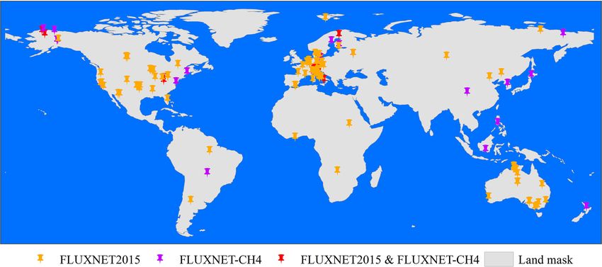
This study used the FLUXNET eddy covariance observations shape parameter of the Gaussian function. Sunrise and sun-
that cover all continents; this includes the FLUXNET2015 set times were calculated using the National Oceanic and At-
(Pastorello et al., 2020) and FLUXNET-CH4 community mospheric Administration (NOAA) solar calculations (https:
products (Knox et al., 2019). FLUXNET2015 contains 212 //www.esrl.noaa.gov/gmd/grad/solcalc/calcdetails.html, last
observation sites from 1991 to 2014, while the FLUXNET- access: 3 August 2021). Subsequently, the sine and Gaussian
CH4 community product contains 81 sites from 2006 to function upscaling methods may be described as follows:
2018. The longest observational record was 25 years, while 1 Ptn
the shortest record was less than 1 year. Half-hourly data se- n t=t0 SINEt
LEd = LEi , (4)
ries on LE, Rs , Rn , and ground heat flux (G) were used for SINEt
the upscaling schemes, while the observed air temperature, 1 P tn
t=t0 GAUSSIANt
wind speed, atmospheric pressure, vapor pressure deficit, LEd = n LEi , (5)
GAUSSIANt
crop heights, observation height of wind, and humidity data
were used in the Penman–Monteith equation. All missing where LEd is the simulated daily LE during the daytime, and
values were eliminated; for example, if there were miss- LEi is the instantaneous LE used in the simulation. The LEt
ing values on a certain day, all data on that day were dis- was calculated using Eqs. (2) and (3) for the sine and Gaus-
carded. As such, only days with fully available half-hourly sian functions, respectively.
data were used in the analysis. Then, only sites with a data The EF and ETrF methods assume a constant ratio be-
series longer than 360 d were used. These eliminations ul- tween LE and the upscaling variable; this may be described
timately meant a total of 122 FLUXNET2015 sites and 42 as follows:
FLUXNET-CH4 sites were used in the analysis due to the LEd LEi
lack of observations (Table S1). There were 16 sites belong- = , (6)
Vd Vi
https://doi.org/10.5194/hess-25-4417-2021 Hydrol. Earth Syst. Sci., 25, 4417–4433, 2021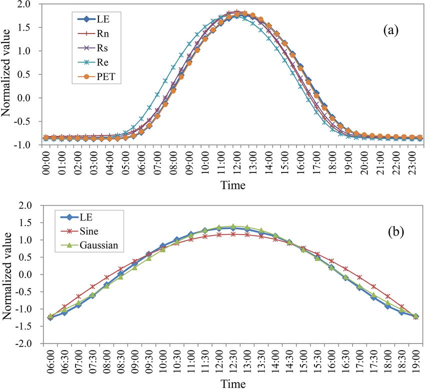
4420                                        Z. Liu: The accuracy of temporal upscaling of instantaneous evapotranspiration

Figure 1. Location of eddy covariance observations.

where LEi and LEd are the instantaneous and daytime LE,                 The daily LE, derived from Eq. (6), may also be simulated
respectively, and Vi and Vd are the instantaneous and daily          as follows:
upscaling variables, respectively.                                           Vd
   The four EF methods involve the upscaling variables,              LEd =      LEi .                                           (9)
                                                                             Vi
Rn , Rn -G, Rs and Re ; the former three variables are mea-
sured by FLUXNET. Re , which is also known as the top-of-            For the EF(Rn ), EF(Rn -G), and EF(Rs ) methods, V is the
atmosphere solar irradiance, is calculated by the following          observed Rn , Rn -G, and Rs , respectively. For EF(Re ) and
equation (Ryu et al., 2012):                                         EF(PET), V is calculated from Eqs. (7) and (8), respectively.
                                                                   When the absolute value of Vi is extremely low, the observed
                             2π DOY
Re = Ssc × [1 + 0.033 cos             ] cos β,          (7)          or calculated Vi in Eq. (9) may generate an anomaly in the
                              Ydmax                                  Vd /Vi ratio. This will produce an abnormally high simulated
where Ssc is the solar constant (1360 W m−2 ); DOY is the            LEd ; as such, abnormal Vd /Vi ratios (i.e., > 10) were dis-
day of the year; Ydmax is the maximum number of days (365            carded in the simulation.
or 366) for the specified year; β is the specific time-of-day
                                                                     2.3   Sky conditions
solar zenith angle calculated using the NOAA solar calcula-
tions.                                                               The daily atmospheric transmissivity coefficient (τ ), calcu-
   The ETrF method involves the upscaling variable, PET,             lated as the ratio of incoming shortwave radiation to extrater-
herein referred to as EF(PET); PET is calculated using the           restrial radiation, was used to represent the sky conditions;
Penman–Monteith equation (Penman, 1948; Monteith, 1981;              this is indicative of daily atmospheric transmissivity. The hy-
Allen et al., 1998):                                                 pothesis is that during clear-sky conditions, shortwave in-
        1 (Rn − G) + ρa cp (es −e a)                                 coming radiation is strongly correlated with extraterrestrial
ρλE =                      ra ,                             (8)    radiation, although it deviates in cloudy conditions. The daily
            1 + γ 1 + rras                                           τ is calculated as follows (Baigorria et al., 2004; Wandera et
                                                                     al., 2017):
where ρ is the density of water; λ is the latent heat of va-
porization, which is the unit conversion coefficient between               Rsd
                                                                     τ=        ,                                               (10)
ET and LE; 1 is the slope of the saturation vapor pressure–                Red
temperature relationship; (Rn -G) is the available energy flux;      where Rsd and Red are the observed daily incoming short-
ρa is the mean air density at constant pressure; cp is the spe-      wave radiation and calculated top-of-atmosphere solar irra-
cific heat of the air; (es − ea ) represents the vapor pressure      diance (in MJ m−2 d−1 , converted from W m−2 ) during the
deficit of the air; γ is the psychometric constant; and rs and       daytime, respectively.
ra are the surface and aerodynamic resistances, respectively.
The calculation of 1, ρa , cp , γ , rs , and ra follows the method   2.4   Evaluation criteria
specified in Allen et al. (1998), in which additional observa-
tions of air temperature wind velocity, atmospheric pressure,        The accuracy of the seven upscaling methods was evalu-
vegetation height, and observation heights of wind and hu-           ated using homogeneous datasets across a range of tem-
midity are required.                                                 poral scales and variable sky conditions. The criteria used

Hydrol. Earth Syst. Sci., 25, 4417–4433, 2021                                           https://doi.org/10.5194/hess-25-4417-2021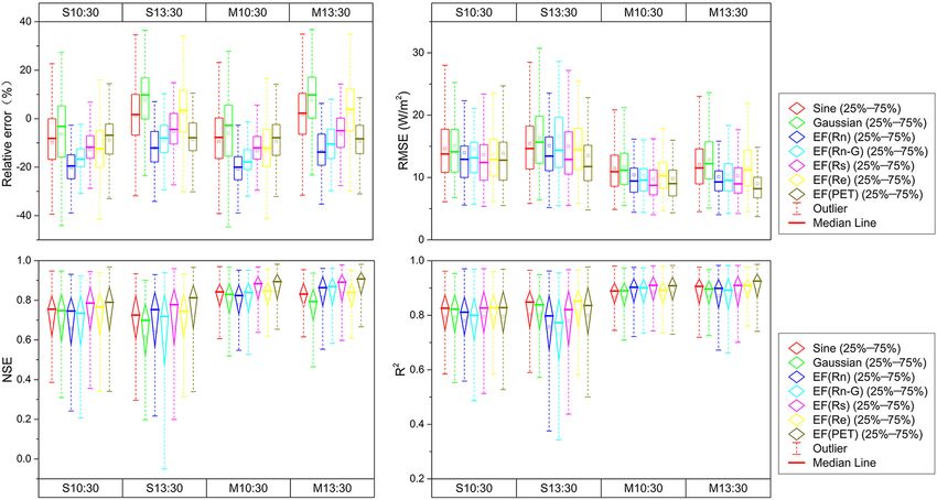
Z. Liu: The accuracy of temporal upscaling of instantaneous evapotranspiration                                                    4421

to evaluate these methods included the relative error (RE),
root-mean-square error (RMSE), Nash–Sutcliffe efficiency
(NSE), and determination coefficient (R 2 ). The RE and
RMSE represented bias deviation from observed values,
while NSE and R 2 are indicative of the goodness of fit of
the simulated and observed data series. The best fit value was
1.0, while the goodness of fit deteriorated with increasing de-
viation from 1.0. The evaluation criteria were calculated as
follows.
      1 Xn Xmi − Xoi
RE =       i=1
                           ,                               (11)
      n            Xoi
         r
            1 Xn
RMSE =           i=1
                     [(Xmi − Xm ) − (Xoi − Xo )]2 ,        (12)
            n
            Pn
                  (Xmi − Xoi )2
NSE = 1 − Pi=1                 2 ,                        (13)
               n
               i=1 X  oi − X o
          Pn
                (Xmi − f (i))2
R 2 = 1 − Pi=1               2 ,                          (14)
             n
             i=1 Xmi − Xm
                                                                   Figure 2. Intra-day distribution of normalized LE, Rn , Rs , Re , and
where Xmi and Xoi are the ith values of the modeled and            PET and the values from the sine and Gaussian functions.
observed LE time series, respectively; n is the length of a
time series; Xm and Xo are the means of the modeled and
observed LE, respectively; and f (i) is a linear fitted function   the afternoon and tended to overestimate LE from 06:00 to
between the observed and modeled daily LE series.                  10:00 and from 15:00 to 17:00.

                                                                   3.2   Accuracy of seven upscaling methods in simulating
3     Results                                                            daily LE series

3.1    Intra-day distribution of observed LE and its               Figure 3 presents the results from evaluating the daily LE
       influencing variables                                       simulations using the seven remote sensing ET upscaling
                                                                   methods, which include the sine and Gaussian functions,
The intra-day distribution characteristics of each flux vari-      EF(Rn ), EF(Rn -G), EF(Rs ), EF(Re ), and EF(PET). The per-
able were analyzed based on the field observation data. Fig-       formance of each upscaling scheme while simulating the
ure 2 shows the intra-day distribution of half-hourly LE, Rn ,     mean value shows that daily LE simulated by most schemes
Rs , Re , and PET, derived from the mean of 148 FLUXNET            was lower than the observed values, where the underestima-
sites. LE was stable and showed little variance from 20:00         tion was generally less than 20 %. Among them, the sine and
to 06:00. During this period, LE accounted for only 5.4 %          Gaussian function methods demonstrated a relatively better
of the total daily LE, while it showed unimodal distribution       performance for the mean values, where the RE was gen-
from 06:00 to 19:00. Factors that directly or indirectly af-       erally within ±10 %. The Gaussian and sine functions also
fected LE, including Rn , Rs , Re , and PET, exhibited a sim-      performed the best in simulating the mean daily LE at 10:30
ilar intra-day distribution to that of LE. Among them, the         and 13:30, respectively. The mean values of daily LE sim-
intra-day distribution of PET demonstrated the best agree-         ulated by the EF(PET) method were also relatively closer
ment with the measured LE (Fig. 2a). However, the intra-day        to measured values. The EF(Rn ) method exhibited the poor-
distributions of Rn , Rs , and Re showed an overall deviation      est performance for mean daily LE simulation of all upscal-
from that of the measured LE. The distribution of Rn and           ing schemes. The simulated RE using this method generally
Rs was generally half an hour earlier than the measured LE,        ranged from 0 % to −40 %, with the mean RE of all sites be-
while that of Re was 1 h earlier. The intra-day distribution of    ing approximately −20 %. In general, there was only a small
the observed LE from 06:00 to 19:00 was compared with the          difference between upscaling simulations using the single-
sine and Gaussian functions (Fig. 2b). The results showed          time value and those using multi-time values. However, the
that daytime LE was more consistent with the latter than the       mean of simulated daily LE by the upscaling schemes at
sine function, which is commonly used to upscale instanta-         13:30 was significantly higher than that at 10:30. The mean
neous ET to daily values in remote sensing applications. The       REs of all upscaling schemes for the former and latter time
Gaussian function matched LE perfectly at any time during          points were −2.3 % and −9.7 %, and the corresponding me-
the day. The sine function slightly underestimated LE during       dian REs were −1.8 % and −9.2 %, respectively. As such,

https://doi.org/10.5194/hess-25-4417-2021                                        Hydrol. Earth Syst. Sci., 25, 4417–4433, 2021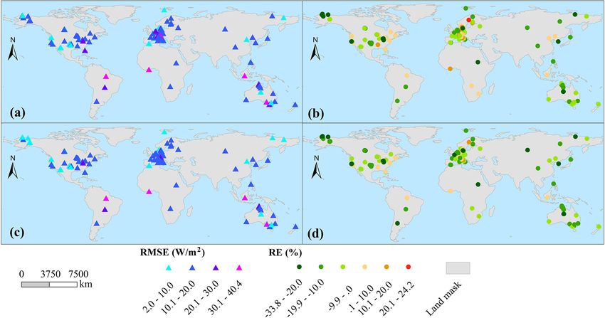
4422                                     Z. Liu: The accuracy of temporal upscaling of instantaneous evapotranspiration

the mean daily LE upscaled from 13:30 was closer to the          methods were 11.0 and 10.3 W m−2 . In terms of the eval-
measured value than that from 10:30; the performance of up-      uation results of the correlation index R 2 , in general, there
scaling methods was better at 13:30 than at 10:30.               was little difference between the performance of the seven
    The RMSE evaluation showed that the RMSE of each             methods. The mean R 2 at each site was 0.87, and the corre-
upscaling scheme at each site ranged from 5 to 30 W m−2 ,        sponding median was 0.90.
where the mean of all simulated RMSEs was 13.5 W m−2 .              Based on this comprehensive evaluation, while the
In the RMSE evaluation, there was only a small difference        EF(PET) method was the most optimal of all seven meth-
between the upscaling simulations at 10:30 and 13:30, as         ods, it also had the greatest input data requirements. The sine
opposed to the RE evaluation results. However, the sim-          function, Gaussian function, and EF(Re ) methods, which re-
ulation accuracy of multi-time values was slightly higher        quired the least input data, also produced relatively accu-
than the single-time value. The mean RMSEs of all up-            rate simulations. Among them, the Gaussian function method
scaling schemes for the former and latter were 15.0 and          demonstrated the best performance for the mean value sim-
11.7 W m−2 , while the corresponding median values were          ulation. The EF(Re ) method was similar to the PET method
13.8 and 10.5 W m−2 , respectively.                              as per the RMSE, NSE, and R 2 , with a larger RE range.
    Figure 3 also presents the evaluations based on the NSE
and R 2 data series criteria, which evaluate the goodness of     3.3   Spatial distribution of the accuracy of the sine
fit of the simulated and observed data series. In general, all         function and EF(Re ) methods
upscaling schemes could accurately simulate daily LE series.
The median NSE and R 2 were generally higher than 0.70 and       In general, all upscaling methods demonstrated an ability to
0.80 for all sites under each upscaling scheme, respectively.    accurately simulate daily LE data series at most sites, par-
This means that the daily LE series simulated by each upscal-    ticularly for simulations using multi-time values. The spatial
ing scheme was relatively consistent with observed values        distribution of the accuracy of the sine function and EF(Re )
and was strongly correlated with the measured data series.       methods simulated using multi-time values was evaluated
Similarly to the RMSE evaluation, simulations using multi-       using NSE and R 2 (Fig. 4). The NSE of the sine function
time values were more accurate than those using a single-        (134/148) and EF(Re ) (133/148) methods was higher than
time value. For example, when a single-time value is used in     0.60 at 90 % of sites worldwide. There were 86 and 90 sites
upscaling schemes, the simulated NSE of each site mainly         that had an NSE exceeding 0.80 for the sine function and
fell between 0.60 and 0.80. In contrast, when multi-time val-    EF(Re ) methods, respectively. In terms of the correlation
ues were used for simulations, the NSE of each site increased    evaluation criterion, R 2 , the number of sites in which the R 2
to between 0.70 and 0.90, where the median exceeded 0.80.        exceeded 0.80 was 117 and 121 for the two methods, respec-
In single-time value simulations, the median of the simulated    tively.
R 2 of all sites was approximately 0.80; when multi-time val-       Notably, in tropical rainforest (e.g., BR-Sa3, GH-Ank, ID-
ues were used, the R 2 improved to a value exceeding 0.90.       Pag) and tropical monsoon (PH-RiF) climatic conditions, the
There was a minor difference between the 10:30 and 13:30         two methods demonstrated a poor ability to simulate daily
upscaling schemes based on the NSE and R 2 evaluation cri-       LE. This was particularly the case for tropical rainforest cli-
teria. This is because the upscaling scheme assumes that the     mate regions, where the NSE is even lower than 0; this may
intra-day distribution of the upscaling variable is similar to   be due to irregular changes in the LE in these regions. For
that of the observed LE. Therefore, the upscaling scheme can     example, there is little seasonal variation in LE in tropical
successfully simulate daily LE at any time during the day.       rainforest climate regions, and the fluctuation of daily LE
However, there was significant variability in the accuracy of    data series is relatively small. This results in poor agreement
upscaling methods when simulated in the evening or night-        between simulated daily LE and measured values (Fig. 5).
time.                                                            However, the SD-Dem site, also located near the Equator,
    A comparative analysis of the different upscaling methods    was characterized by seasonal variation in LE due to the
was also performed. The daily LE data series simulated by        tropical grassland climate in this region. As such, the sim-
the EF(PET) and EF(Rs ) methods showed a relatively greater      ulated daily LE at this site demonstrated greater consistency
level of consistency with observed values than those simu-       with measured values. Although the performance of upscal-
lated by the other five methods. For example, in simulations     ing methods was poor in agreement with the daily LE data,
of multi-time values, the mean and median NSE simulated          there was an apparent correlation between simulated daily
by the two methods at each site were 0.83 and 0.89, while        LE and the measured data. For example, the R 2 was higher
the corresponding values simulated by the other five meth-       than 0.30 and 0.40 at the GH-Ank and ID-Pag sites, respec-
ods were 0.77 and 0.84, respectively. The RMSE evaluation        tively, while it was greater than 0.50 at the PH-RiF site.
results were similar to those for NSE. For example, in sim-         The spatial distribution of the accuracy of the sine function
ulations of multi-time values, the mean and median RMSEs         and EF(Re ) methods simulated by multi-time values was also
simulated by the two methods were 9.8 and 8.9 W m−2 , re-        evaluated using the RE and RMSE criteria (Fig. 6). The sim-
spectively, while the corresponding values for the other five    ulated RE at all sites ranged from −33.7 % to 24.2 %, while

Hydrol. Earth Syst. Sci., 25, 4417–4433, 2021                                     https://doi.org/10.5194/hess-25-4417-2021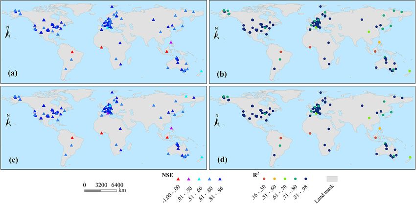
Z. Liu: The accuracy of temporal upscaling of instantaneous evapotranspiration                                                        4423

Figure 3. Simulation accuracy of daily LE using seven remote sensing ET upscaling methods, including the sine and Gaussian functions,
EF(Rn ), EF(Rn -G), EF(Rs ), EF(Re ), and EF(PET). Note: S and M represent simulations by a single and average of multi-time values,
respectively. For example, S10:30 is simulated by the ratio of a daytime value to a single-time value at 10:30, while M10:30 is simulated by
the ratio of a daytime value to the average of three-time values at 10:00, 10:30, and 11:00.

Figure 4. Spatial distribution of NSE and R 2 simulated by the sine function and EF(Re ) methods with multi-time values (a and b are
simulated by the sine function method, and c and d are simulated by the EF(Re ) method; a and c are NSE, and b and d are R 2 ).

the RMSE was lower than 40.4 W m−2 . Most sites tended                  region of South America, both methods generally overesti-
to underestimate daily LE using the two upscaling meth-                 mated daily LE by less than 10 %. Both methods tended to
ods; this underestimation was generally less than 20 %. In              underestimate the daily LE in the remaining regions by less
East Asia, central Australia, northeastern Africa, central and          than 10 %. The simulated RMSE of the upscaling methods
northwestern North America, and southern South America,                 exceeded 30 W m−2 at three tropical rainforest sites and a
the upscaling methods underestimated daily LE by 10 %–                  site in southeastern Australia. The remaining sites had RMSE
20 %. In the Gulf of Guinea in Africa and the northeastern

https://doi.org/10.5194/hess-25-4417-2021                                             Hydrol. Earth Syst. Sci., 25, 4417–4433, 2021
4424 Z. Liu: The accuracy of temporal upscaling of instantaneous evapotranspiration
simulated NSE had improved to exceed 0.70, and the corre-
sponding R 2 was greater than 0.75. This indicates that re-
mote sensing ET upscaling methods can achieve satisfactory
simulation accuracy even when 0.4 < τ < 0.5. The simula-
tion accuracy of the two methods was relatively stable when
τ > 0.6, particularly for the EF(PET) method of multi-time
values at 13:30 in which the corresponding NSE stabilized
around 0.85, and R 2 was stable around 0.87. The RE also
became relatively stable when τ > 0.6; this is consistent with
the R 2 results, as shown in Fig. 8a and b. This indicates that
the daily LE simulated by the sine function and EF(PET) up-
scaling methods was closer to the measured values, and the
simulation accuracy of these methods was high and more re-
liable when τ > 0.6. The accuracy evaluation results of the
other upscaling methods were similar (not shown).
Overall, under sky conditions where τ > 0.6, the upscaling
schemes could simulate the daily LE series with high accu-
racy. However, when τ < 0.6, this simulation accuracy was
significantly affected by sky conditions and was generally
positively correlated with the daily atmospheric transmissiv-
Figure 5. Observed and simulated daily LE series by the sine func- ity coefficient. Although not as accurate as when atmospheric
tion upscaling method in tropical regions. Note: (a) to (c) represent transmissivity is high (τ > 0.6), the upscaling schemes still
BR-Sa3, GH-Ank, and ID-Pag, located in the tropical rainforest cli-
demonstrated an ability to accurately simulate daily LE even
mate region; (d) and (e) are the sites of PH-RiF and SD-Dem, lo-
cated in the tropical monsoon and grassland climate regions, respec-
when atmospheric transmissivity was relatively low (i.e.,
tively. 0.4 < τ < 0.5).
In addition to the overall evaluation of the data series con-
structed across all sites, the performances of different sites
values below 30 W m−2 . There were 89 % (132/148) of sites under all sky conditions were evaluated. Figure 8a and b
with a simulated RMSE lower than 20 W m−2 . show the R 2 when using the sine function and EF(PET)
methods under differing daily atmospheric transmissivity
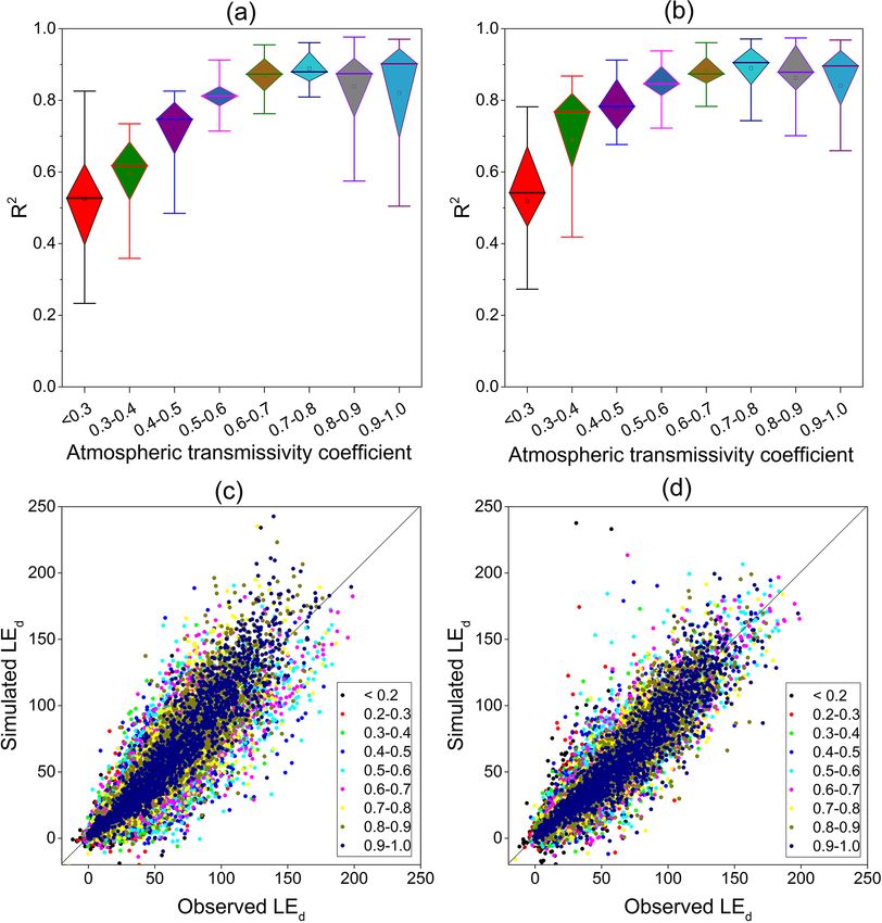
3.4 Accuracy of upscaling schemes in simulating daily coefficients. In general, the R 2 of the upscaling methods
LE under all sky conditions increased with the atmospheric transmissivity coefficient;
when τ > 0.6, the simulation accuracy was stable. Based on
In this study, the simulation accuracy of upscaling meth- the evaluation of the EF(PET) method with multi-time val-
ods under a different daily atmospheric transmissivity coef- ues at 13:30, when τ < 0.3, the R 2 of each site was mainly
ficient (τ ) was evaluated using observed data from sites with between 0.4 and 0.7. When τ increased to between 0.3 and
a daily time series length greater than 1000. First, all data 0.4, the R 2 had increased to between 0.6 and 0.8 at most
from these sites were constructed into a data series. Then, sites. When τ > 0.6, the R 2 of each site generally increased
the accuracy of daily LE simulations using the sine function to greater than 0.8. Figure 8c and d show the simulated daily
and EF(PET) upscaling methods under differing daily atmo- LE against observed values under different levels of daily at-
spheric transmissivity coefficients was evaluated; the results mospheric transmissivity; the simulation systematically un-
are presented in Fig. 7. In general, the simulation accuracy derestimates the simulations with observed values under low
was positively correlated with the daily atmospheric trans- levels of τ (i.e., τ < 0.2). For the instant simulation in up-
missivity coefficient, particularly when τ < 0.6. The overall scaling schemes, it is important to note that simulations may
RE, RMSE, NSE, and R 2 were 6.0 % and 9.1 %, 14.3 and be upscaled from instantaneous variables when the sky is
11.8 W m−2 , 0.81 and 0.86, and 0.83 and 0.88 for the sine cloudy, while the remainder of the daytime is clear. However,
function method using the single-time value at 10:30 and the opposite may also occur in which the sky conditions are
the EF(PET) method using the multi-time values at 13:30, clear during instant simulation and cloudy at other times.
respectively. The simulation accuracy under sky conditions
where τ < 0.6 was significantly lower than the overall ac- 3.5 Accuracy of upscaling schemes in simulating daily
curacy. For example, when τ < 0.2, the two methods under- LE from different times of day
estimated the daily LE by 36.7 % and 25.0 %, respectively.
Although the simulation accuracy was not as high as that Remote sensing ET upscaling was conducted based on the
under large atmospheric transmissivity, the simulated NSE monitoring value of the satellite overpass time; the overpass
exceeded 0.50, even when τ < 0.2. When 0.4 < τ < 0.5, the times of different satellites may vary in different regions.
Hydrol. Earth Syst. Sci., 25, 4417–4433, 2021 https://doi.org/10.5194/hess-25-4417-2021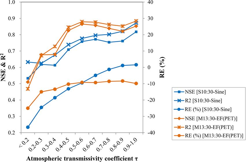
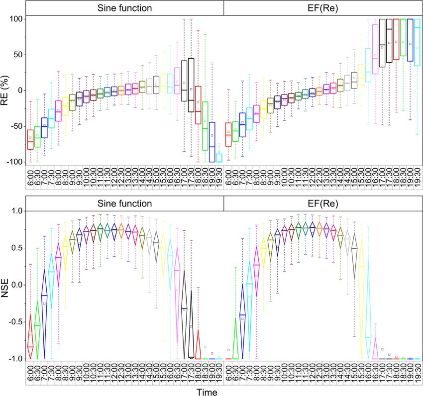
Z. Liu: The accuracy of temporal upscaling of instantaneous evapotranspiration                                                        4425

Figure 6. Spatial distribution of RE and RMSE simulated by the sine function and EF(Re ) methods using multi-time values (a and b are
simulated by the sine function method, and c and d are simulated by the EF(Re ) method; a and c are RMSE, and b and d are RE).

Figure 7. Overall evaluation of the sine function method simulated
by a single-time value of 10:30 and the EF(PET) method simulated
by multi-time values at 13:30 for all sites under differing daily at-
mospheric transmissivity coefficients.

Therefore, the simulation accuracy of the temporal upscal-
ing methods was also evaluated at different times of the day.
Figure 9 presents the RE and NSE of the simulations using               Figure 8. Box plots showing the R 2 of the (a) sine function method
the sine function and EF(Re ) methods at different times of             simulated by a single time at 10:30 and the (b) EF(PET) method
the day; these two methods required minimal input data. In              simulated by multi-time values at 13:30 for each site. Scatter plots
general, the simulation accuracy of the sine function method            between observed and simulated daily LE by the (c) sine function
had initially increased and then decreased during the day-              and (d) EF(PET) methods under differing daily atmospheric trans-
time. Before 09:00, the mean RE for all sites increased lin-            missivity coefficients.
early from −65.8 % to −14.9 %, and the RE varied signifi-
cantly at each site. For example, the RE at each site ranged
from −80 % to 30 % when the simulation was upscaled at

https://doi.org/10.5194/hess-25-4417-2021                                             Hydrol. Earth Syst. Sci., 25, 4417–4433, 2021
4426                                        Z. Liu: The accuracy of temporal upscaling of instantaneous evapotranspiration

Figure 9. RE and NSE of simulated daily LE using the sine function and EF(Re ) methods at different times of the day.

08:00. From 09:00 to 16:30, the mean RE for all sites was              ing daily LE data series also showed significant variability
also increasing, although the magnitude of this increase was           at different times of the day. The intra-day variation of NSE
significantly reduced, increasing from −14.9 % to 13.0 %.              based on two methods at different times of the day may also
During this period, the performance of the upscaling method            be divided into three distinct stages: (1) a general linear in-
was relatively stable, particularly during 11:00–14:00, where          crease before 10:00, (2) a period of relative stability from
the RE at each site was mainly distributed from −20 % to               10:00 to 13:30, and (3) a general linear decrease after 14:00.
20 %. However, from 17:00, the mean RE showed a sharper                During (1), the mean NSE of all sites increased from be-
decrease, and the performance of the upscaling method be-              low −0.60 to 0.60 and 0.61 for the sine function and EF(Re )
came extremely unstable at each site; this meant the RE var-           methods, respectively, while the median NSE increased from
ied significantly at each site. The daily LE was overestimated         below −0.80 to 0.73 for both methods. The two methods
by more than 90 % at some sites, while it was also underes-            showed the highest simulation accuracy for 10:00–13:30. In
timated by more than −90 % at other sites. With respect to             each single time point, the mean and median NSEs of all sites
the EF(Re ) method, the RE generally showed an increasing              based on the sine function method were 0.65 and 0.74, while
trend during the daytime. There were three distinct stages.            the corresponding values using the EF(Re ) method were 0.66
(1) From 06:00 to 09:00, the mean RE at all sites increases            and 0.76, respectively. In addition, most sites had an NSE
linearly from −57.6 % to −20.5 %. (2) From 09:00 to 14:30,             higher than 0.5 at single time points of 09:00, 09:30, 14:00,
the mean RE was also increasing, although at a lower rate              and 14:30. This indicates that the two methods also produce
from −20.5 % to 10.5 %. (3) After 15:00, the mean RE ex-               a certain accuracy in simulating daily LE at a single time
hibits a sharp linear increase from 17.5 % to 60.3 % at 17:00          point, as the mean NSE of all sites was approximately 0.50
and then always exceeds 60 % thereafter.                               and the corresponding median exceeded 0.60. However, the
   According to the NSE evaluation criterion, the accuracy of          simulation accuracy of the two methods was relatively poor
the sine function and EF(Re ) upscaling methods in simulat-            in the remaining periods, with a mean and median NSE lower

Hydrol. Earth Syst. Sci., 25, 4417–4433, 2021                                            https://doi.org/10.5194/hess-25-4417-2021
Z. Liu: The accuracy of temporal upscaling of instantaneous evapotranspiration 4427
than 0.50, particularly before 08:00 and after 16:00; in these The variability of simulation accuracy among different
periods, the NSE for most sites was lower than 0.20 or even sites was evaluated through the site-to-site standard devia-
lower than 0. In other words, the two methods lose the ability tion of NSE, as shown in Fig. 10b. In each upscaling scheme,
to upscale instantaneous LE to daily data series during these the site-to-site standard deviation of data series composed
periods. of NSE for every site (where the length of each series is
Overall, the accuracy of the sine function and EF(Re ) up- 122, equal to the number of sites) ranged from 0.21 to 0.28,
scaling methods in simulating daily LE exhibits significant while the mean and median NSE of all upscaling schemes
variability during the daytime. The simulation accuracy of was 0.25. In each case, the variability of simulation accuracy
both methods was relatively high from 09:00 to 15:00, with among different sites was greater than that among upscal-
the mean REs at all sites within ±20 % and the mean and ing schemes as the site-to-site standard deviation was always
median NSEs being higher than 0.50 and 0.60, respectively. larger than the standard deviation among upscaling schemes.
In particular, from 11:00 to 13:30, the simulation accuracy of This higher site-to-site standard deviation is mainly due to
the two methods was relatively high and stable at each site. the extremely low NSEs at several individual sites (as shown
The RE of each site was within ± 20 %, and the mean and in Fig. 4). The site-to-site standard deviation significantly re-
median NSEs were 0.65 and 0.74, respectively. However, the duces if we exclude the four sites with an NSE lower than
two methods lose the ability to accurately simulate daily LE 0.5. For example, when only considering sites with an NSE
data during other times of the day, exhibiting poor simulation greater than 0.5 (118), the site-to-site standard deviation is
accuracy. Evaluation of the simulation accuracy for the other mainly distributed between 0.10 and 0.15, with mean and
upscaling methods (not shown) at different times of the day median values of 0.12. The site-to-site standard deviation
was generally consistent with those of the sine function and falls below 0.09 in each upscaling scheme, when only 66
EF(Re ) methods, supporting the conclusions of this study. sites with an NSE greater than 0.8 were used to calculate the
site-to-site standard deviation. The corresponding mean and
median values of the standard deviation were 0.06. Overall,
3.6 Variability of simulation accuracy among different
the variability of simulation accuracy among different sites
upscaling schemes and sites
was mainly affected by a limited number of sites with an ex-
tremely low NSE. Indeed, the large variations in simulation
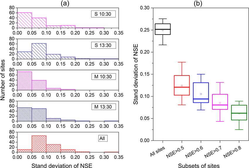
Based on data from 122 sites from FLUXNET2015, the stan- accuracy among different upscaling schemes with a standard
dard deviation of the NSE was used to evaluate the vari- deviation of NSE exceeding 0.20 (Fig. 10a) occurred at these
ability of simulation accuracy among the different upscal- four sites.
ing schemes and sites (Fig. 10). For remote sensing ET up-
scaling, the variability of simulation accuracy among differ-
ent upscaling schemes is typically lower than the variability 4 Discussion
among different sites. At the same site, the mean standard
deviation of data series composed of NSE by each upscaling In the temporal upscaling of instantaneous remote sensing
scheme (the length of each series is 28, equal to the number ET to daily values, the current methods focus only on day-
of upscaling schemes) was 0.096. The standard deviation of time ET. In other words, the upscaling methods only result
the NSE by each scheme was lower than 0.20 at most sites in an ET during the daytime and do not include nocturnal
(119/122). There were 63 % of sites (77/122) with a stan- ET. As for the difference in upscaled daytime LE and daily
dard deviation of less than 0.10; these were the results for values, typically, a correction coefficient corrects this devia-
all upscaling schemes examined in this study. For the seven tion. For example, Gentine et al. (2007) introduced a constant
methods within each type of upscaling scheme (e.g., S10:30, correction factor of 1.1 into the EF upscaling method; this re-
S13:30, M10:30, or M13:30 shown in Fig. 10a), the vari- duced systematic underestimation and improved the perfor-
ability of simulation accuracy among different methods was mance of the method in terms of accuracy and bias for daily
even lower, whereby the standard deviation of NSE in each ET estimates (Ryu et al., 2012; Van Niel et al., 2012). In
scheme was less than 0.10, at more than 75 % of sites. For addition, time-dependent correction factors may further im-
the simulation of multi-time values at 10:30, the standard de- prove EF performance (Van Niel et al., 2011); this was also
viation of NSE among the sine and Gaussian functions and validated by the results of this study. The observation of LE
EF(Rn ), EF(Rn -G), EF(Rs ), EF(Re ), and EF(PET) methods at 148 global sites from FLUXNET shows that the percent-
averaged only 0.052, and the number of sites with a standard age of nocturnal LE to daytime LE ranges from −2.8 % to
deviation of less than 0.10 was up to 112 (92 %). This indi- 19.6 %, with an average of 7.8 %. The correction coefficient
cates that the variability of simulation accuracy among dif- was calculated according to the half-hourly observed LE data
ferent upscaling schemes was relatively small for upscaling series at each site; this coefficient is equal to 1 plus the ratio
instantaneous remote sensing ET to daily values. In addition, of nocturnal LE to daytime LE. The results show that the sim-
the variability of the simulation accuracy when using multi- ulation accuracy with the correction coefficient was slightly
time values was lower than that using the single-time value. higher than that without the correction coefficient. As such,
https://doi.org/10.5194/hess-25-4417-2021 Hydrol. Earth Syst. Sci., 25, 4417–4433, 20214428 Z. Liu: The accuracy of temporal upscaling of instantaneous evapotranspiration Figure 10. Standard deviation of NSE based on (a) different methods and (b) different sites. Note: in the left-hand-side figure, S and M represent different methods by the single- and multi-time values, respectively; “All” contains all upscaling schemes used in this study. In the right-hand-side figure, the site-to-site standard deviations of simulated NSE for every upscaling scheme are shown as columns of a box plot. The five columns represent all sites where the average NSE for all upscaling schemes is higher than 0.5, 0.6, 0.7, and 0.8, and the corresponding numbers of sites are 122, 118, 111, 97, and 67, respectively. when LE observation data become available, the correction observation site. This is more consistent with the actual situa- coefficient should be used to correct the simulation of daily tion at each site than the reference ET. However, the greatest LE in the remote sensing ET upscaling schemes. However, disadvantage of this method is that it requires the input of hourly LE observation data are seldom available in the ac- multiple observational datasets, such as air temperature, hu- tual application of remote sensing ET upscaling; as such, it midity, wind speed, atmospheric pressure, crop height, and is necessary to consider the simulation accuracy of upscaling observation height. It should be noted that FLUXNET in- schemes without hourly LE data support. Therefore, the eval- cludes both raw and corrected LE data. There was little dif- uation results presented in this study were simulations with- ference between the evaluation results of the corrected data out any correction coefficients. In addition, note that even in and those of the raw data. the absence of LE observational data, a correction coefficient The sine function and EF(Re ) methods may be more suit- of 1.08 on the average global sites may be used to correct able for regional remote sensing applications due to their rel- daily LE simulated by these upscaling methods. atively simpler inputs and comparable or higher accuracies The evaluation results show that the simulation accuracy when compared to other methods. This is consistent with the of these different methods varied based on the evaluation in- conclusions of other studies (Zhang and Lemeur, 1995; Liu dex used. The comprehensive evaluation results show that the and Hiyama, 2007; Van Niel et al., 2012; Ryu et al., 2012). simulation accuracy using the EF(PET) method was the best Compared with the sine function, the intra-day distribution among all seven upscaling methods. Previous studies often of LE was more consistent with the Gaussian function. How- used reference evapotranspiration as PET in EF(PET) upscal- ever, in terms of the overall performance of upscaling meth- ing schemes (Trezza, 2002; Colaizzi et al., 2006; Allen et al., ods, the simulation accuracy of the Gaussian function for 2007; Cammalleri et al., 2014). The reference crop is defined daily LE did not show significant improvement. This may be as a hypothetical crop with an assumed height of 0.12 m, a mainly caused by the complementary effect between the un- surface resistance of 70 s m−1 and an albedo of 0.23 (Allen derestimation of the sine function method around 12:00 and et al., 1998). However, PET is related to differences in the the overestimation of the method in the morning and after- aerodynamic properties between the reference surface and noon. This results in an upscaled LE in the daytime by the the actual landscape around the flux measurement site. In this sine function, which is similar to that of the Gaussian func- study, PET was calculated by considering the parameters of tion. the (bulk) surface and the aerodynamic resistance for water The upscaling variable originally used by the EF method vapor flow based on the actual vegetation conditions at each was Rn -G (Sugita and Brutsaert, 1991); in general, G is neg- Hydrol. Earth Syst. Sci., 25, 4417–4433, 2021 https://doi.org/10.5194/hess-25-4417-2021
Z. Liu: The accuracy of temporal upscaling of instantaneous evapotranspiration                                                4429

ligible in the daily energy balance (Price, 1982; Li et al.,        There was little seasonal variation in LE in tropical rainforest
2009; Cui et al., 2020). However, for the application of the        climate regions, and the fluctuation range of daily LE data
EF method to upscale instantaneous ET to a daily scale, the         was relatively small. This may be one of the causes of the
instantaneous value of G is required. As Rn is also recom-          poor simulation accuracy of daily LE in these regions. Al-
mended in the EF upscaling method (Brutsaert and Sugita,            though the performance of upscaling schemes was in poor
1992), the EF(Rn ) method has been validated at several sites.      agreement with the daily LE series, it indeed showed a rough
For example, Van Niel et al. (2012) showed that EF(Rn ) un-         correlation between the simulated and measured daily LEs at
derestimated monthly ET by −16 % at two sites in Australia;         these tropical rainforest and tropical monsoon sites.
the magnitude of underestimation was lower than that sim-              Delogu et al. (2012) used four European flux sites to eval-
ulated by the EF(Rn -G) method (−34 %). In this study, the          uate the performance of the EF(Rn -G) and EF(PET) meth-
performance of the EF(Rn ) and EF(Rn -G) methods in up-             ods at different times from 10:00 to 14:00, finding that the
scaling LE at 148 global sites with a long data series (includ-     simulation accuracy at 11:00–13:00 was slightly higher than
ing seasonal variations) was compared. The results showed           outside of this time range. Based on the 126 FLUXNET
that there was little difference between the simulation accura-     sites from 1999 to 2006, Wandera et al. (2017) evaluated the
cies of the EF(Rn ) and EF(Rn -G) methods; this may be good         EF(Rs ) method at different times between 10:30 and 14:00
news for remote sensing ET applications. Compared to Rn , G         and found that there was only slight variance in the accu-
is very difficult to detect using remote sensing (Kalma et al.,     racy of daily LE simulations during this period. However,
2008; Li et al., 2009), as it is usually calculated from the em-    the performance of upscaling methods during other daytime
pirical relationship between Rn and land surface parameters         periods has seldom been investigated. In this study, the per-
(Bastiaanssen et al., 1998; Su et al., 2002; Li et al., 2019). In   formance of seven upscaling methods at different times dur-
addition, due to the combined errors in Rn and G, the avail-        ing the day (06:00–19:00) was evaluated; the simulation ac-
able energy (Rn -G) error estimated by remote sensing meth-         curacy of upscaling methods was observed to vary signifi-
ods can reach ±10 %–20 % (Bisht et al., 2005; Kalma et al.,         cantly during the day. The upscaling methods were only able
2008). However, if LE is only upscaled for the winter, ignor-       to simulate daily LE with relatively high accuracy between
ing the effect of G may produce large errors in the simulation      09:00 and 15:00. All the methods lost their ability to accu-
(Cammalleri et al., 2014).                                          rately simulate daily LE outside of these hours. The upscal-
    In any upscaling scheme, the simulation accuracy of multi-      ing methods exhibited the highest simulation accuracy from
time values is clearly higher than that of a single-time value,     11:00 to 14:00. This is consistent with previous results (De-
which may be due to better stability in the Vd /Vi ratio (Eq. 8)    logu et al., 2012; Wandera et al., 2017). Overall, in upscal-
offered by the former than the latter. It is recommended that       ing instantaneous ET to daily values in remote sensing appli-
multi-time values are used in remote sensing ET upscaling           cations, instantaneous values between 11:00 and 14:00 are
when multi-time data are available. For example, if mete-           recommended for simulations. However, if the simulation is
orological observations are selected as upscaling variables,        upscaled from a time outside of 09:00–15:00, simulation ac-
an upscaling scheme based on multi-time values is recom-            curacy cannot be guaranteed.
mended for simulations.                                                The performance of remote sensing ET upscaling schemes
    The spatial distribution of the simulation accuracy of each     may vary significantly under different sky conditions. Wan-
upscaling scheme showed that most sites could accurately            dera et al. (2017) analyzed the performance of the EF(Rs )
upscale instantaneous LE to daily values. However, sites lo-        method for four different classes of daily atmospheric trans-
cated in tropical rainforests and tropical monsoon regions          missivity, including 0.25 ≥ τ ≥ 0, 0.50 ≥ τ ≥ 0.25, 0.75 ≥
performed poorly in accurately simulating daily LE, with an         τ ≥ 0.50, and 1 ≥ τ ≥ 0.75, where the first class represented
NSE lower than 0.20. This is consistent with the results re-        a high degree of cloudiness and the fourth class represented
ported by Ryu et al. (2012), who assumed that the poor per-         clear skies. They found a relatively better simulation ac-
formance in tropical rainforest regions was mainly due to ir-       curacy for the atmospheric transmissivity class above 0.75.
regular cloudiness. In addition, remote sensing products only       In this study, a more refined classification of daily atmo-
sense the top of the canopy and thus ignore the energy stor-        spheric transmissivity and a greater number of upscaling
age within the canopy. Especially for forest this can be sig-       methods were evaluated. The results showed that the upscal-
nificant (Jiménez-Rodríguez et al., 2020; Coenders-Gerrits          ing methods can simulate daily LE series with high accuracy
et al., 2020). This partially explains the poor performance         at τ > 0.6. When τ < 0.6, the simulation accuracy of each up-
in tropical rainforest regions. The performance of the up-          scaling method was significantly affected by sky conditions;
scaling schemes under all sky conditions was evaluated us-          accuracy was observed to be generally positively related to
ing various daily atmospheric transmissivities. High atmo-          daily atmospheric transmissivity. However, it was also found
spheric transmissivity represents a clear-sky condition with        that the upscaling methods could accurately simulate daily
little cloudiness. However, the simulation accuracy of these        LE series even when the atmospheric transmissivity was rel-
tropical rainforests and tropical monsoon regions under con-        atively low (i.e., 0.4 < τ < 0.5).
ditions of high atmospheric transmissivities was also low.

https://doi.org/10.5194/hess-25-4417-2021                                        Hydrol. Earth Syst. Sci., 25, 4417–4433, 2021
You can also read