Drivers of benthic metacommunity structure along tropical estuaries - Nature
←
→
Page content transcription
If your browser does not render page correctly, please read the page content below
www.nature.com/scientificreports

            OPEN           Drivers of benthic metacommunity
                           structure along tropical estuaries
                           Andreia Teixeira Alves1*, Danielle Katharine Petsch2 & Francisco Barros                    1

                           Community structure of many systems changes across space in many different ways (e.g., gradual,
                           random or clumpiness). Accessing patterns of species spatial variation in ecosystems characterized by
                           strong environmental gradients, such as estuaries, is essential to provide information on how species
                           respond to them and for identification of potential underlying mechanisms. We investigated how
                           environmental filters (i.e., strong environmental gradients that can include or exclude species in local
                           communities), spatial predictors (i.e., geographical distance between communities) and temporal
                           variations (e.g., different sampling periods) influence benthic macroinfaunal metacommunity structure
                           along salinity gradients in tropical estuaries. We expected environmental filters to explain the highest
                           proportion of total variation due to strong salinity and sediment gradients, and the main structure
                           indicating species displaying individualistic response that yield a continuum of gradually changing
                           composition (i.e., Gleasonian structure). First we identified benthic community structures in three
                           estuaries at Todos os Santos Bay in Bahia, Brazil. Then we used variation partitioning to quantify
                           the influences of environmental, spatial and temporal predictors on the structures identified. More
                           frequently, the benthic metacommunity fitted a quasi-nested pattern with total variation explained by
                           the shared influence of environmental and spatial predictors, probably because of ecological gradients
                           (i.e., salinity decreases from sea to river). Estuarine benthic assemblages were quasi-nested likely for
                           two reasons: first, nested subsets are common in communities subjected to disturbances such as one
                           of our estuarine systems; second, because most of the estuarine species were of marine origin, and
                           consequently sites closer to the sea would be richer while those more distant from the sea would be
                           poorer subsets.

                           Understanding how community structure of many systems changes across space and how mechanisms, driven
                           mostly by dispersal and environmental filters, determine species distribution patterns in local communities is
                           a central question in community ecology1–3. Testing how community assembly mechanisms determine species
                           distribution has also become important in metacommunity ecology, an offshoot of community ecology, which
                           has emerged to describe processes occurring at local and regional scales1,4. A metacommunity can be defined as
                           a set of local communities potentially, but not necessarily, linked by the dispersal of multiple, likely interacting,
                           species5,6. Assessing processes that affect metacommunity composition particularly in ecosystems characterized
                           by strong environmental gradients is important to provide useful information on species responses to environ-
                           mental changes across ecological gradients.
                               To understand patterns of spatial variation in species composition, two different and complementary meta-
                           community approaches have been proposed7: one focusing on patterns7,8 and another focusing on mechanisms1,9.
                           The pattern-based approach evaluates the characteristics of species distributions along environmental gradients
                           (i.e., random, checkerboard, nested subsets, evenly-spaced, Gleasonian, or Clementsian patterns)7,8 (Table 1).
                           The mechanistic approach considers the roles of niche (i.e., environmental filters and biotic interactions) and
                           dispersal-related processes in determining such metacommunity structures. Both approaches have provided
                           insights into the different processes that structure communities across different ecosystems10–13, but have not
                           been applied along well-defined ecological gradients.
                               The framework devised by Leibold and Mikkelson8 to identify patterns of metacommunity structure (later
                           expanded7) is based on evaluating three metrics – coherence, turnover and boundary clumping (known as

                           1
                            Laboratório de Ecologia Bentônica, Programa de Pós-Graduação em Ecologia: Teoria, Aplicação e Valores, Instituto
                           de Biologia & CIENAM, Universidade Federal da Bahia, Rua Barão de Geremoabo s/n., Campus Ondina, CEP 40170-
                           115, Salvador, BA, Brazil. 2Núcleo de Pesquisas em Limnologia, Ictiologia e Aquicultura (Nupelia), Programa de
                           Pós-Graduação em Ecologia de Ambientes Aquáticos Continentais (PEA), Universidade Estadual de Maringá, Av.
                           Colombo 5790, CEP 87020–900, Maringá, PR, Brazil. *email: dea_alves106@yahoo.com.br

Scientific Reports |   (2020) 10:1739 | https://doi.org/10.1038/s41598-020-58631-1                                                            1
www.nature.com/scientificreports/                                                                        www.nature.com/scientificreports

                            Pattern          Reference         Description                                                  Processes
                                                                                                                            Biotic process may prevent
                                                               Combinations of mutually exclusive species that occur
                            Checkerboard     Diamond 1975                                                                   coexistence of particular sets of
                                                               independently of other pairs along the gradient.
                                                                                                                            species that interact antagonistically.
                                                                                                                            Species-specific characteristics, such
                                             Patterson and     Species-poor communities are subsets of species-richer
                            Nested subsets                                                                                  as dispersal ability and tolerance to
                                             Atmar 1986        communities.
                                                                                                                            abiotic conditions.
                                                               Groups of species show similar responses to environmental Biotic process may prevent
                            Clementsian      Clements 1916     gradients, which replace each other as a group, and can be coexistence of particular sets of
                                                               classified into distinctive community types.               species that interact antagonistically.
                                                                                                                            Idiosyncratic responses to abiotic
                                                               Communities are structured along some gradient, but
                                                                                                                            factors, with coexistence resulting
                            Gleasonian       Gleason 1926      species display individualistic responses that yield a
                                                                                                                            from change similarities in
                                                               continuum of gradually changing composition.
                                                                                                                            requirements or tolerance.
                            Evenly spaced                      Species are distributed more uniformly than expected by
                                             Tilman 1982                                                                    Strong interspecific competition.
                            gradients                          chance.
                                                               There are no gradients or other patterns in species
                            Random           Simberloff 1983                                                                Indicator of stochastic processes.
                                                               distribution among sites.

                           Table 1. Six idealized structures to identify species distribution among sites. Patterns represent idealized
                           characteristics hypothesized as a result of ecological processes. References indicates early description of
                           these patterns, Description explains each pattern, and Processes is a potentially important ecological or
                           biogeographical cause.

                           Elements of Metacommunity Structure, herein called EMS) – calculated from a presence–absence matrix8,14.
                           Coherence, the first element of the hierarchical EMS framework, is related to the level at which species respond
                           to the same environmental gradient, while turnover relates to the way species composition changes across com-
                           munities, and boundary clumping measures the level of distinctiveness of blocks of species. Following coherence,
                           turnover and boundary clumping, it is possible to identify species’ distribution patterns among sites (Fig. 1).
                           Accordingly, EMS analyzes multiple models simultaneously, comparing them against each other to assess which
                           one best fits a particular metacommunity pattern along a single major ordination axis (i.e., a latent environmental
                           gradient) in the data7,8,10,15. Among the idealized structures for identifying species distributions among sites, com-
                           munity structure can change across space in many different ways (e.g., gradual, random, clumpiness) (Table 1).
                           However, EMS indicates but does not directly inform the processes underlying patterns, such as the role of envi-
                           ronmental filtering or dispersal effects in metacommunity structuring2,4. Therefore, combining the EMS approach
                           with variation partitioning techniques (environmental and spatial variation) is strongly recommended to assess
                           the main drivers of observed metacommunity structure3. For instance, different functional groups of freshwater
                           benthic invertebrate communities12 may display Clementsian or random patterns (identified by the pattern-based
                           approach) likely due to different causes (identified by the mechanistic approach), respectively environmental
                           heterogeneity and dispersal mode.
                               Strong environmental gradients, like salinity gradients in estuaries, may be important metacommunity struc-
                           ture drivers, generating non-random and ecologically meaningful patterns3,10,16. Such gradients can be under-
                           stood as environmental filters that can include or exclude species, at different sites along the gradient, through
                           species interactions with the physical and chemical characteristics of the environment3,17. Environmental filters
                           may be more pronounced than dispersal limitation or interactions between species in environments with strong
                           environmental gradients. Furthermore, spatial variation plays an important role on the arrangement of envi-
                           ronmental gradients and consequently on communities’ final distribution, but there is still a lack of formal tests
                           on strong gradients that include spatial information when analyzing metacommunity structure patterns3,10,12,18.
                           Temporal variation, such as sampling periods, should also be taken into account in metacommunity studies, since
                           communities are not static, but dynamic16,19,20, notably in estuaries21,22. In addition, the relative roles of different
                           local and regional processes in determining community structure and metacommunity pattern remain unclear
                           in estuaries.
                               Estuarine systems are characterized by their transitional position between marine and freshwater ecosystems,
                           which can generate strong and well-defined gradients (i.e., salinity and sediment grain size)23,24. It is well known
                           that benthic communities play important roles in estuaries and, considering that component species have sed-
                           entary or relatively low mobility habits, changes in environmental gradients are frequently detected in benthic
                           organisms resulting in benthic community changes23. Hence, the environmental estuarine gradient along with the
                           benthic community life mode represents an opportunity to explore metacommunity patterns. Also, knowing the
                           type of structure and the drivers shaping metacommunities in estuaries is important for providing information
                           on how species respond to salinity gradients and, consequently, on the underlying mechanisms responsible for
                           the general functioning of these systems21,26,27. Thus, estuaries are highly productive systems and provide several
                           goods and services as they are often used as feeding areas and nursery grounds by various species, and serve as
                           natural pollution filters and storm buffers21,24. However, despite their high ecological and economic importance,
                           estuaries experience a wide array of human impacts, such as increased urbanization and industrialization and
                           altered connection to marine and freshwater systems due to shoreline development25. These influences can com-
                           promise their ecological integrity and consequently change the structure of benthic assemblages. Environmental
                           condition changes in systems characterized by strong gradients such as estuaries may reflect alterations in species
                           replacement9,22, and impacts over time might modify the organisms’ ranges along the salinity gradient23, high-
                           lighting the importance of knowing how such communities are structured and the main drivers of structure.

Scientific Reports |   (2020) 10:1739 | https://doi.org/10.1038/s41598-020-58631-1                                                                                    2
www.nature.com/scientificreports/ www.nature.com/scientificreports
Figure 1. Schematic representation used to examine how the EMS (i.e., coherence, turnover and boundary
clumping) results in six main metacommunity structures (i.e., checkerboards, random, nested, evenly spaced,
Gleasonian and Clementsian) and quasi-structures. S = significant; NS = non-significant; “ + ” = positive;
“−” = negative; “I” = Morisita’s index value. Modified from Presley et al.7 and Brasil et al.65.
We used an empirical framework linking the EMS approach and variation partitioning (environmental, spatial
and temporal variation)3 to understand the emergence of benthic macroinfaunal metacommunity structure along
salinity gradients in tropical estuaries. Even though benthic species diversity patterns along tropical estuaries21,22
(decreasing from marine to freshwater zones) had challenged previous well-accepted paradigms (i.e., Remane,
193428), metacommunity patterns of estuarine species are still unclear. This study offers insight into the debates
on diversity patterns along estuaries through a metacommunity approach. We first expected a Gleasonian pattern
(i.e., species displaying individualistic responses producing a continuum of gradually changing composition),
since estuarine benthic fauna had been previously associated with ecocline23 and species replacement22 ideas.
Thus, we predicted that the benthic metacommunity would be organized according to salinity preferences21–23 fol-
lowing a non-clumped association (i.e., Gleasonian distribution). Due to the strong salinity gradient, we expected
environmental filters to be more important in explaining benthic community variation than were spatial and
temporal predictors.
Materials and Methods
Study area. We conducted our study in the estuarine portion of the three main tributaries of Todos os Santos
Bay located in Bahia state in Brazil: Paraguaçu (56,300 km2), Subaé (600 km2) and Jaguaripe (2,200 km2) Rivers29
(Fig. 2). Several anthropogenic activities, such as industrial effluents, untreated sewage, urbanization, agriculture,
ports and mining activities, have decreased the environmental quality in some specific regions of our study area30.
Since we were interested in analyzing the influence of environmental filters on the structure of metacommunities,
each estuary studied encompassed the effect of a salinity gradient ranging from approximately 0.5 to 40 along
10 or 11 randomly chosen stations (Fig. 3). Each one of the 10 (Jaguaripe and Paraguaçu) or 11 stations (Subaé)
along the salinity gradient had two randomly chosen sites. A total of 270 sites were sampled for all estuarine
systems over time. In each estuary, we sampled in a gradient from the most seaward and generally deepest sta-
tion (i.e., lower-numbered stations in Fig. 2) to the furthest inland and shallowest station (i.e., higher-numbered
stations in Fig. 2).
The survey took place over time in different estuaries. The Subaé estuary was sampled in five periods: Jun-
2004, Mar-2006, Dec-2009, Apr-2011, and Mar-2013. The Jaguaripe estuary was sampled in four periods: May-
2006, Aug-2007, Jul-2010, and Aug-2014. Finally, the Paraguaçu estuary was sampled in four periods: May and
Dec-2005, Jun-2011, and Aug-2014.
Sample collection and processing. In the Paraguaçu estuary, the six replicates were collected at each
station using a van Veen grab (0.05 m2, 3.2 L). In Subaé and Jaguaripe, at each station eight replicates were col-
lected manually by divers, using corers (10 cm diameter, 0.008 m2, 1.2 L). Core sampling was not suitable in the
Paraguaçu River due to the depth at some stations ( > 35 m), very strong water current and zero visibility. For
both types of gear, sample infauna was collected from the water–sediment interface to a depth of 15 cm31. All
macroinfaunal samples were sieved through a 0.5 mm mesh in the field, preserved in 70% alcohol and taken to the
Scientific Reports | (2020) 10:1739 | https://doi.org/10.1038/s41598-020-58631-1 3www.nature.com/scientificreports/ www.nature.com/scientificreports
Figure 2. Map of the study area showing sampled stations (black dots) for each estuary (Subaé, Jaguaripe, and
Paraguaçu) at Todos os Santos Bay, in Bahia, Brazil.
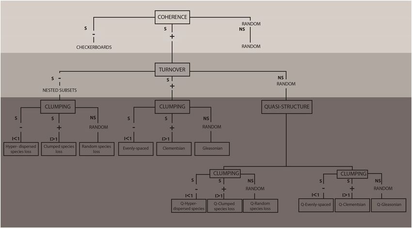
Figure 3. Salinity gradient from sea to freshwater in sampled sites for Jaguaripe (circles), Paraguaçu (triangles)
and Subaé (squares) estuaries at Baía de Todos os Santos.
laboratory for further processing and identification. Most invertebrates were identified to family level; family has
been shown to be a taxonomically sufficient descriptor of estuarine benthic invertebrates in habitats with strong
gradients32 but still provide information about community identities and their temporal drift33. Also, family level
was a good choice due to the scarcity of taxonomical studies of the local benthic invertebrates (with several unde-
scribed species) and allowed comparison of the taxon distribution patterns observed in other regions21.
The environmental variables measured included salinity and sediment type (i.e., grain size). Salinity of the
superficial water was measured at spring low ebb tides and recorded using a Hydrolab Data Sonde. One sediment
sample was collected at each station for grain size analysis, using a 0.05 m2 van Veen grab for Paraguaçu River
and a 0.008 m2 corer for Subaé and Jaguaripe. Sediment particle size was determined by standard techniques34.
Salinity and each fraction of sediment grain size (i.e., pebble, gravel, very coarse sand, coarse sand, medium sand,
fine sand, very fine sand and silt sand clay) were treated as environmental predictors.
Sample adequacy. In order to evaluate whether the benthic macroinfaunal family of each estuary was rep-
resentatively sampled and to avoid artifactual patterns because the probability of detection of species varied, we
calculated the relationship between sampling effort and family richness for each estuary for the total sampling
time. The specaccum function and the species accumulation method random were used in the vegan package35
Scientific Reports | (2020) 10:1739 | https://doi.org/10.1038/s41598-020-58631-1 4www.nature.com/scientificreports/ www.nature.com/scientificreports
in the R environment36. Sample-based rarefaction is preferable than individual-based rarefaction to account for
natural levels of sample heterogeneity in the data37.
A total of 11,328 individuals of benthic invertebrates were sampled, mainly belonging to 144 taxa of
Polychaeta, Mollusca and Crustacea. Polychaeta was the most abundant phylum, followed by Mollusca and
Crustacea. In spite of differences in the sampling methods (i.e., sampling gear, total area sampled, number of
sites and replicates) among estuaries, most of the systems showed a near stabilization of the relationship between
number of stations and richness, allowing further analyses (Supplementary Fig. 1).
Elements of metacommunity structure. We used incidence matrices (i.e., presence–absence) to esti-
mate Elements of Metacommunity Structure (EMS). We followed the ‘range perspective’ in our analysis, which is
defined by species range turnover and range boundary clumping8 as recommended38. These incidence matrices
were subsequently subjected to a reciprocal averaging (also known as Correspondence Analysis, CA), an uncon-
strained ordination method, which positions sites having similar species composition close to each other and
locating species having similar occurrence among the sites close to each other along the ordination axis39. Because
we focused only on the first ordination axis, other ordination methods, such as detrended correspondence analy-
sis, will give the same results8. When a single or at least a predominant gradient structures a community data set,
the reciprocal averaging arranged matrix will display this gradient effectively.
Coherence, the first EMS metric, is based on calculating the number of embedded absences (i.e., interrup-
tions in species distribution or in the composition of the sites) in the ordinated matrix and then comparing the
empirical observed value of embedded absences (EmbAbs) to a null distribution created from simulated matrices
with 1,000 iterations7,8. A large number of embedded absences (i.e., EmbAbs significantly larger than expected
by chance) suggests negative coherence and leads to a checkerboard distribution of species; non-significant
coherence refers to a random metacommunity type; and a small number of embedded absences (i.e., EmbAbs
significantly lower than expected by chance) suggests positive coherence related to nestedness, evenly spaced,
Gleasonian or Clementsian gradients8 (Fig. 1).
Turnover is evaluated if coherence is significant and positive (Fig. 1). It is measured by the number of times
one species replaces another between two sites (i.e., number of replacements) in an ordinated matrix. To do this,
the number of empirical replacements (turnover) was compared to the distribution of randomly generated values
based on a null model distribution that randomly shifts entire ranges of species8. Significant negative turnover
(i.e., replacement significantly lower than expected by chance) refers to nested subsets, while significant posi-
tive turnover (i.e., replacement significantly larger than expected by chance) refers to evenly spaced gradients
(Gleasonian or Clementsian structures), requiring further analysis of boundary clumping to distinguish among
them8. Furthermore, cases where coherence is significant and positive and turnover is non-significant can be
regarded as quasi-structures, indicating that the effects of structuring mechanisms are weaker than in idealized
structures7 (Fig. 1).
Boundary clumping is analysed using the Morisita’s Index40 and a chi-square test comparing observed and
expected distributions of range boundary locations. Non-significant clumping, and values of Morisita’s index that
are not different from 1, indicate randomly distributed species loss in nested subsets when turnover is negative
or Gleasonian distribution when turnover is positive. Values significantly larger than 1 indicate clumped species
loss in nested subsets when turnover is negative or Clementsian distribution when turnover is positive. Values
significantly less than 1 indicate hyperdispersed species loss in nested subsets when turnover is negative and an
evenly spaced metacommunity type when turnover is positive (Fig. 1).
The significance of coherence and turnover was tested separately using the fixed-proportional null model,
where the species richness of each site was maintained (i.e., row sums were fixed), but species frequencies of
occurrence (i.e., columns) were filled based on their marginal probabilities. Random matrices were produced
by the r1 method using the R package vegan35 for the fixed-proportional null model, which has a more desirable
combination of Type I and Type II error properties7 and has been applied successfully15,16,38,41,42. All EMS analyses
were done using the metacom package43 in the R environment (version 1.5.0)36.
Nestedness. We performed ‘nestedness metric based on overlap and decreasing fill’ (NODF)44 to accurately
identify nestedness along salinity gradients in estuarine benthic communities. There is some criticism about the
EMS framework used to investigate idealized metacommunity patterns and especially whether the turnover test is
adequate for detecting a nested pattern, as turnover and nestedness are not necessarily exclusive or opposite38,45,46.
Schmera et al.46 showed that even though high turnover is frequently related to low nestedness, low turnover does
not predict high nestedness. We performed NODF using the oecosimu function from the vegan package35 in the
R environment (version 2.0-10)36.
Spatial predictors. We used Principal Components of Neighbour Matrices (PCNM) to generate spatial var-
iables from geographical coordinates (e.g., latitude and longitude) represented as a Euclidean distance matrix47,48.
The PCNM technique represents the spatial configuration of sample points using principal coordinates of a trun-
cated geographic distance matrix between sampling sites. We used the resulting PCNM eigenvectors associated
with the positive eigenvalues as spatial components in a global test and in a forward selection prior to variation
partitioning47,49,50. PCNM analyses were done using the function pcnm in the vegan package35 in the R environ-
ment (version 2.0-10)36.
Environmental predictors. We converted environmental data to standardized Z-scores by subtracting each
environmental variable from their mean and dividing by their standard deviation. The new standardized variables
are thus dimensionless, with a mean of 0 and a standard deviation of 151. In addition, we tested multicollinearity
using a variance inflation factor (VIF)52. When the VIF values indicated a high level of collinearity, we removed
Scientific Reports | (2020) 10:1739 | https://doi.org/10.1038/s41598-020-58631-1 5www.nature.com/scientificreports/ www.nature.com/scientificreports
the predictor with the highest VIF value. We then recalculated VIF and repeated this process until all VIFs were
below a pre-selected threshold (VIF < 3)52,53. Standardized Z-score and VIF analyses were done using the func-
tions scale and vif.cca, respectively, in the vegan package35 in the R environment (version 2.0-10)36.
Variation partitioning. We used partial Redundancy Analysis (pRDA)51 to quantify the pure and shared
contributions of environmental filters (i.e., salinity and each fraction of sediment grain size), spatial variables
(i.e., variables created using PCNM) and time (i.e., sampling occasions) structuring the benthic metacommunity
in the estuaries. RDA can be best understood as an extension of multiple regression that has multiple response
variables (i.e., species) and a common matrix of predictors (i.e., environmental and spatial predictors)54. pRDA
or variation partitioning51 may indicate the relative strength of association between each component and the
metacommunity pattern of benthic macroinvertebrates. We expected environmental variables to be the main
influencer of benthic metacommunity structure. In situations where environmental gradients determine most of
the variation in the living community, the amount of variation in species data explained by environmental vari-
ables is fairly high55. We also included sampling period as a temporal predictor in variation partitioning because
time may influence community structure, but we did not have specific expectations regarding temporal variation
in benthic structures.
Prior to the pRDA, we Hellinger-transformed abundance matrices and report values based on adjusted R2 to
provide unbiased estimates of explained variation and valid comparisons between sets of factors for explaining
community structure54. Hellinger transformation consists of transforming the site-by-species data into relative
values per site by dividing each value by the site sum, and then taking the square root of the resulting values42. It
is suitable for community composition data in comparative analysis because it reduces the importance of high
species abundance.
We first did a global RDA test to prevent the inflation of Type I error, and only if it was significant proceeded
with forward selection using the double-stopping criterion: the usual alpha significance level (p < 0.05) and the
adjusted coefficient of multiple determination (R2)49. Each eigenvector was counted as a single predictor since this
approach is the most conservative in its penalization of degrees of freedom and adjusted R2 statistics50. We used
forward selection to determine the environmental and spatial filters to be used in variation partitioning. Forward
selection analyses for spatial and environmental predictors were done using the ordiR2step function in the vegan
package35 in the R environment (version 2.0-10)36.
We carried out pRDA using the function varpart in the vegan package35 in the R environment (version 2.0-
10)36. We report adjusted R2 and test the significance of the pure environmental, pure spatial and pure temporal
components (P < 0.05). The total percentage of variation explained by the model (R2) is partitioned into unique
and common contributions of sets of predictors54. It offers a way of dealing with the importance of spatial corre-
lation when observations are not independent, the number of degrees of freedom in the sample is smaller than
expected based on the number of observations used in the analysis, and Type I errors increase, leading to incor-
rect conclusions about the effect of the environment on community structure56. Statistical significance of RDA in
global models was based on 999 permutations and assessed at a significance level of 0.05.
Results
Elements of metacommunity structure. The EMS analysis indicated five metacommunity patterns
among the six idealized patterns57–62 and the quasi-structures7 (Table 2). We found that the Q-nested (n = 6)
metacommunity type structure was the most common followed by nested (n = 3), Q-Clementsian (n = 2),
Clementsian (n = 1), and Q-Gleasonian (n = 1) (Supplementary Fig. 2). As expected, for all estuaries the first
step of EMS analysis (Fig. 1), indicated that metacommunity structure was positively coherent (P < 0.001).
That is, EmbAbs was significantly lower than expected by chance (Table 2) likely due to the salinity gradient
(Supplementary Fig. 2). The second EMS step (Fig. 1) revealed that turnover was not significant (P > 0.05) in most
cases (9 out of 13), displaying quasi-structures7 and predominantly negative turnover. That is, replacement was
lower than expected by chance) (Table 2) (Supplementary Fig. 2). Even though spatial turnover among sites was
more often linked to environmental gradients49, these results indicated that benthic macroinfaunal metacommu-
nities did not always follow a species replacement structure. Finally, the boundary clumping third step (Fig. 1),
showed that Morisita’s index was higher (P < 0.005) than 1 for most (11) of the cases, indicating positive clumping
structures or clumped species loss for the Q-nested and nested structures (Supplementary Fig. 2).
Nestedness. NODF results suggested that in Subaé and Paraguaçu systems, benthic macroinfaunal meta-
community followed an intermediate nested distribution for while the Jaguaripe system had a highly nested
structure (Supplementary Table 1). Taxa vs. sites occurrence resulting from the overall NODF analysis based on
incidence matrices along salinity gradients for Todos os Santos Bay estuarine systems showed that most of the
taxa found follow Q-nested and nested species composition (Fig. 4).
Variation partitioning. The RDA used in the spatial global model was significant for all estuaries (Subaé:
adjusted R2 = 0.28, P < 0.001; Jaguaripe: adjusted R2 = 0.48, P < 0.001; Paraguaçu: adjusted R2 = 0.26, P < 0.001),
so forward selection was carried out to select spatial variables among PCNM eigenvectors associated with the
positive eigenvalues before variation partitioning (Table 3).
The multicollinearity test for environmental predictors for all systems did not show a high VIF value for
salinity even before dropping the predictor with the highest VIF value, indicating that there was no problem of
multicollinearity among salinity and other predictors. However, sediment predictors showed a high VIF value
and the predictor with highest value (VIF < 3) was removed for each system (Subaé: coarse sand, granular gravel,
and silt/clay; Jaguaripe: fine sand, very coarse sand, and silt/clay; Paraguaçu: coarse sand, granular gravel and
silt/clay). The remaining variables had a VIF value smaller than the threshold (Supplementary Table 2). The
Scientific Reports | (2020) 10:1739 | https://doi.org/10.1038/s41598-020-58631-1 6www.nature.com/scientificreports/ www.nature.com/scientificreports
Coherence Turnover Boundary clumping
Sim Sim
Estuary Month Year embAbs Coh Z P mean Sim sd Turnover Tur Z P mean Sim sd Index P df Interpretation
Subaé 03 2013 95 6.52 < 0.001 179 13 921 −0.37 0.716 875 126 1.04 0.267 8 Q-Gleasonian
Subaé 04 2011 94 3.14 < 0.001 131 12 537 1.10 0.271 658 111 1.41 0.008 8 Q-nested*
Subaé 12 2009 101 7.58 < 0.001 280 24 886 6.01 < 0.001 2228 2229 4.29 0.001 8 Nested*
Subaé 03 2006 57 7.26 < 0.001 196 19 962 2.94 < 0.001 1296 117 1.20 0.107 8 Nested#
Subaé 06 2004 36 8.54 < 0.001 130 11 911 1.55 0.123 1095 119 4.00 0.001 7 Q-nested*
Jaguaripe 08 2014 85 1.06 < 0.001 210 12 2103 −0.27 0.787 2024 290 2.08 0.001 7 Q-Clementsian
Jaguaripe 07 2010 104 6.07 < 0.001 193 15 1150 1.25 0.204 1374 179 1.73 0.009 7 Q-nested*
Jaguaripe 08 2007 98 6.79 < 0.001 184 13 1058 0.36 0.721 1113 156 1.74 0.008 7 Q-nested*
Jaguaripe 05 2006 35 5.71 < 0.001 749 7 339 −1.10 0.270 287 47 1.74 0.002 6 Q-Clementsian
Paraguaçu 08 2014 263 1.01 < 0.001 392 13 3895 0.99 0.320 4270 378 1.36 0.001 6 Q-nested*
Paraguaçu 06 2011 130 1.18 < 0.001 288 14 3481 0.37 0.715 3651 469 1.95 0.003 7 Q-nested*
Paraguaçu 12 2005 91 1.13 < 0.001 253 15 2195 258 < 0.001 2852 255 1.99 0.008 7 Nested#
Paraguaçu 05 2005 89 1.01 < 0.001 229 14 1886 −2.02 < 0.05 1527 177 1.35 0.001 7 Clementsian
Table 2. The Elements of Metacommunity Structure results for each estuary (Subaé, Jaguaripe and Paraguaçu).
These results were based on the fixed-proportional (r1) null model. Interpretations followed Leibold &
Mikkelson8 and Presley et al.7. Abbreviations: embABS = embedded absences; Coh Z = Z-value of coherence;
Tur Z = Z-value of turnover; Q = Quasi. Significant p-values are indicated by bold font. *Nested clumped speceis
loss (sensu Presley et al.7), Q = Quasi. #Nested random speceis loss (sensu Presley et al.7), Q = Quasi.
environmental global model was significant (Subaé: adjusted R2 = 0.24, P = 0.001; Jaguaripe: adjusted R2 = 0.38,
P = 0.001; Paraguaçu: adjusted R2 = 0.25, P = 0.001), so forward selection of environmental variables was also
carried out to select environmental filters after the removal of collinear explanatory variables (Table 3).
The shared influence of environmental and spatial predictors explained a high proportion of benthic meta-
community structure (Fig. 5). For example, in the Subaé estuary, the shared influence of environmental and
spatial predictors explained 12% of the variance, and spatial factors alone explained 7% (Fig. 5). Similarly, shared
environmental and spatial predictors explained 25% and spatial predictors explained 10% in the Jaguaripe estuary.
(Fig. 5). Finally, in the Paraguaçu estuary, temporal components explained 12% of metacommunity structure fol-
lowed by 11% explained by shared environmental and spatial components (Fig. 5). Purely environmental, purely
spatial and purely temporal predictors were significant (P < 0.01) influences in all three estuaries (Supplementary
Table 3).
Discussion
We used EMS combined with a variation partitioning techniques to identify the relationships between environ-
mental, spatial and temporal predictors structuring benthic metacommunities in estuarine systems. However,
our prediction that benthic macroinfaunal metacommunities would follow a non-clumped associations char-
acterized by a continual change in species composition along environmental gradients without the formation of
discrete assemblages (i.e., Gleasonian distribution) was not supported. Instead, we found Q-nested and nested
species composition with clumped species loss as the most frequent patterns. We also did not corroborate our
prediction of the higher importance of pure environmental filters, but found a higher importance of the shared
fraction between environment and space influencing benthic metacommunity. Therefore, in this system benthic
communities along estuaries were generally subsets of a large pool of species (i.e. nested or Q-nested) and with
space, salinity and sediment size were most strongly associated with this pattern.
Even though we observed six metacommunity types7, the overall metacommunity fitted Q-nested (Q-clumped
species loss) or nested subsets (clumped species loss). Nestedness may arise when sites with lower species richness
are subsets of richer sites as a result of environmental conditions of the habitats or species-specific characteristics,
such as dispersal ability or tolerance of abiotic conditions62. Nested structures are not rare, and they have already
been reported for aquatic metacommunities10,15,20,41,63. Most species found in estuarine systems have marine ori-
gin and diversification23, so the sites closer to the sea are richer while the sites closer to freshwater have poorer
subsets, as fewer estuarine species can arrive and/or survive in such conditions (e.g., lower salinity and depth).
Some taxa, like polychaetes from the families Nereididae and Capitellidae, and also Tellinidae mol-
lusks, showed a wide distribution along all estuarine systems (Fig. 4). However, Chironomidae (Insecta) and
Oligochaeta, for example, are adapted to freshwater systems and occurred only at the sites farthest from the sea
(Fig. 4). This partially explains nestedness being not so strong (Q-nested) and the distinct patterns found on dif-
ferent sampling occasions. Another important consideration is that, at timescales of months and years, the same
taxa might migrate up or down the estuarine gradient in order to physiologically couple with environmental
variability.
The emergence of a Q-Gleasonian gradient occurred only for one sampling period for the Subaé estuary. The
upper zone (more freshwater) of this estuary is well known for its inorganic pollution in the sediments64.Given the
high importance of the strong salinity gradient in estuarine systems, we expected the dominance of Gleasonian
patterns at metacommunity level for all estuarine systems, as a result of species having differential responses to
the environmental gradients. Nevertheless, it seems that a nestedness situation, where most of the taxa can live in
Scientific Reports | (2020) 10:1739 | https://doi.org/10.1038/s41598-020-58631-1 7www.nature.com/scientificreports/ www.nature.com/scientificreports
Figure 4. Taxa vs. sites, incidence matrices along the salinity gradient at the sampled stations for Jaguaripe,
Paraguaçu and Subaé estuaries after ordination according to occurrence resulting from the overall NODF
analysis. Black squares indicates the presence of a taxon, while white squares indicates the absence of a taxon
along the salinity gradient indicated as distance to marine waters (km).
more salty regions (richer sites) and some of them will tolerate different levels of freshwater, is predominant. The
emergence of a Clementsian structure for one sampling period for the Paraguaçu estuary and a Q-Clementsian
structure for two sampling periods for the Jaguaripe estuary was also unexpected. The Clementsian gradient may
be related to historical biogeographic features such as the process of communities’ isolation and/or environmental
variation65 showing that sets of species respond similarly to environmental variation, but the occurrence of envi-
ronmental stochastic stress zones lead to clumped boundaries. Moreover, our study clearly shows that whenever
metacommunity patterns are under investigation it is imperative to have replicates in time and space at landscape
level (e.g., different estuaries, lakes, rivers etc sampled at different times) because such patterns are dynamic.
We observed a high amount of benthic metacommunity variation explained by the shared influence of envi-
ronmental filters and spatial predictors for all estuaries. However, since the variation was not exclusively caused
by spatial variables, we can still argue that environmental filters (i.e. salinity and sediment) are important in
Scientific Reports | (2020) 10:1739 | https://doi.org/10.1038/s41598-020-58631-1 8www.nature.com/scientificreports/ www.nature.com/scientificreports
Estuarine Spatial selected Environmental
system variables selected variables VIF
Salinity 1.72
Medium sand 1.81
Subaé PCNM 1, 3, 2, 5
Fine sand 1.29
Pebble 1.39
Coarse sand 1.92
Salinity 1.70
Jaguaripe PCNM 1, 2
Very fine sand 1.47
Medium sand 1.50
Fine sand 1.78
Paraguaçu PCNM 1, 3, 2
Salinity 2.21
Table 3. Environmental and spatial factors selected through forward selection, after checking multicollinearity
using variance inflation factor (VIF) for each variable, during the sampled periods in the three main tributaries
(Subaé, Jaguaripe and Paraguaçu) at Todos os Santos Bay.
shaping benthic metacommunity structure3. Spatial predictors, measured as geographical distance, were consid-
ered to play a significant role in the similarity of species compositions between sites1. Accordingly, environmental
variables in estuaries, especially salinity, were spatially structured, which may explain why the highest proportion
of total variance was explained by the shared influence of environmental and spatial predictors (Fig. 5). Salinity
decreases according to distance from sea to river (Fig. 3), and consequently may affect benthic metacommunity
structure from high species and feeding-guild diversities to dominance by a single species or a feeding group27
and decrease in diversity at family level21,22.
Communities change dynamically in richness and composition over time, and consequently the underly-
ing mechanisms are not static over time either4,19,20,41. Unlike the other systems, the Paraguaçu estuary had two
sample campaigns in the same year representing two different seasons and it was the system in which variation
partitioning showed temporal predictors as the most important component for explaining total variation. There
is also a possibility that freshwater inflows into the Paraguaçu estuary may have greater variability than would
naturally occur because of construction of the Pedra do Cavalo Dam during the 1980s and the implementation of
the Pedra do Cavalo Hydroeletric Power Plant for energy generation in 200566. Our results suggest that potential
differences between those metacommunity structures (e.g. Paraguaçu Dec-2005 nested vs. Paraguaçu May-2005
Clementsian) and temporal components are worth additional research. We strongly suggest that future stud-
ies should include hypotheses explicitly related to temporal variation (i.e., seasons, drought/flood) with specific
changes in metacommunity patterns.
For the same estuaries sampled in this study, Barros et al.21 found a decrease in diversity of benthic mac-
roinfaunal assemblages, at family level, from marine to freshwater zones. Likewise, Barros et al.22 showed that
α-diversity decreased along marine to freshwater conditions, while β-diversity was driven by replacement or
nestedness depending on the level and distribution of disturbances in estuaries subjected to anthropogenic stress-
ors. Both studies contradict the most popular estuarine model, the Remane model28, which suggests a diversity
minimum zone called the arteminimum.
Contrastingly, environmental disturbances may result in environmental homogenization due to high dis-
persal, which can result in homogenization of metacommunities, increasing nestedness and decreasing species
replacement65,67. The Subaé estuary is well-known to be impacted by human activity, with high levels of inorganic
contaminants in the upper estuary30 and showed a nested pattern for four sampling periods out of five (Table 2).
Jaguaripe and Paraguaçu estuaries also had a decrease in concentrations of contaminants seawards, but they are
considered relatively well conserved. The less disturbed Jaguaripe estuary, displayed less nestedness (in two out
of four sampling periods) than Paraguaçu (three out of four) (Table 2). Nestedness was more often found in the
Subaé estuary, where the upper region (contaminated) is poorer in species richness compared to the lower region,
likely accentuating the nestedness pattern from sea to freshwater.
There is some criticism about the EMS framework used to investigate idealized metacommunity patterns and
especially whether the turnover test is adequate for detecting nested patterns, as turnover and nestedness are not
necessarily mutually exclusive or opposite38,45,46. Nestedness can be measured using various metrics26, such as
NODF, that may not be directly comparable to the one used in the context of the EMS framework. Consequently,
results based on EMS to evaluate nestedness may be inconsistent if compared to these indices, which ordinate
matrices based on richness of sites and species incidence. However, the reciprocal averaging method used in
the EMS analysis for nested subsets discerns inter-site variation in response to a latent environmental gradient
enhancing the association of mechanisms with nested structures and the form of species loss7. Also, if EMS are
studied for a wide range of taxa and locations as in this study, general associations may emerge between particular
idealized patterns of distribution and specific taxa38.
Since nestedness is among the non-random distribution patterns related to species-specific characteristics
such as dispersal ability, habitat specialization and tolerance to abiotic conditions, future studies should integrate
temporal dynamics, spatial predictors and environmental filters with dispersal traits and disturbances in the EMS
approach. Dispersal mode is a regional process considered a strong driver for benthic metacommunity distri-
bution pattern4,11,12,19,67 as more dispersive species are more controlled by the environment than less dispersive
Scientific Reports | (2020) 10:1739 | https://doi.org/10.1038/s41598-020-58631-1 9www.nature.com/scientificreports/ www.nature.com/scientificreports
Figure 5. Explained proportion of variance partitioning for each estuarine system (Subaé, Jaguaripe and
Paraguaçu): the effects related to environmental filters (Env), those related to spatial patterns (Spa), those
resulting from temporal patterns (Time), shared influence of environmental filters and spatial descriptors
(Env + Spa), environmental filters and temporal patterns (Env + Time), and spatial descriptors and temporal
patterns (Spa + Time). Numbers indicate the explained proportion of variation partitioning for each estuarine
system; values = 0 are not shown. **P < 0.01 (Supplementary Table 3).
species60. Considering that many natural systems are subjected to human impacts, such as the upper region of
the Subaé estuary, integrating the knowledge of how local (i.e., environmental filters, geographical distance) and
regional (i.e., dispersal mode) processes structure natural systems may improve management.
Estuaries are strongly impacted by human activities, in addition to natural stressors, which can affect assem-
blage structure affecting the functioning of these important systems26,68. Knowing the type of structure and the
drivers that shape metacommunities along different estuarine gradients and how that structure changes over time
is important for future studies aiming at conservation to help to establish effective conservation policies3,26. Our
study indicated that benthic metacommunities follow Q-nested and nested structures and are highly influenced
by the shared influence of environmental and spatial predictors. We identified many common taxa occurring
across all salinity gradients (e.g., Capitelllidae and Nereididae) as well as the most habitat-specialist taxa, with
occurrence only in more freshwater sites (e.g., Chironomidae and Oligochaeta). More importantly, by studying
a strong environmental gradient at different times we showed that metacommunity patterns will differ since
environmental conditions will vary. We believe our study advances the knowledge on how estuarine benthic
communities are structured. We showed that salinity and proximity (space) are major drivers and also highlighted
the importance of spatial and temporal replication whenever investigating stronger ecological gradients. Future
studies should incorporate functionality and explicit time-related hypotheses.
Received: 3 July 2019; Accepted: 19 January 2020;
Published: xx xx xxxx
References
1. Leibold, M. A. et al. The metacommunity concept: a framework for multi-scale community ecology. Ecol. Lett. 7, 601–613, https://
doi.org/10.1111/j.1461-0248.2004.00608.x (2004).
2. Logue, J. B. et al. Empirical approaches to metacommunities: a review and comparison with theory. Trends Ecol. Evol. 26, 482–491,
https://doi.org/10.1016/j.tree.2011.04.009 (2011).
3. Gascón, S. et al. Environmental filtering determines metacommunity structure in wetland microcrustaceans. Oecologia 181,
193–205, https://doi.org/10.1007/s00442-015-3540-y (2016).
4. Erős, T., Takács, P., Specziár, A., Schmera, D. & Sály, P. Effect of landscape context on fish metacommunity structuring in stream
networks. Freshw. Biol. 62, 215–228, https://doi.org/10.1111/fwb.12857 (2017).
5. Gilpin, M. E. & Hanski, I. A. Metapopulation Dynamics: Empirical and Theoretical Investigations. (Academic Press, London, 1991).
6. Wilson, D. S. Complex interactions in metacommunities, with implications for biodiversity and higher levels of selection. Ecol. 73,
1984–2000, https://doi.org/10.2307/1941449 (1992).
7. Presley, S. J., Higgins, C. L. & Willig, M. R. A comprehensive framework for the evaluation of metacommunity structure. Oikos 119,
908–917, https://doi.org/10.1111/j.1600-0706.2010.18544.x (2010).
8. Leibold, M. A. & Mikkelson, G. M. Coherence, species turnover, and boundary clumping: elements of meta-community structure.
Oikos 97, 237–250, https://doi.org/10.1034/j.1600-0706.2002.970210.x (2002).
9. Cottenie, K. Integrating environmental and spatial processes in ecological community dynamics. Ecol. Lett. 8, 1175–1182, https://
doi.org/10.1111/j.1461-0248.2005.00820.x (2005).
10. Henriques-Silva, R., Lindo, Z. & Peres-Neto, P. R. A community of metacommunities: exploring patterns in species distributions
across large geographical areas. Ecol. 94, 627–639, https://doi.org/10.1890/12-0683.1 (2013).
11. Petsch, D. K., Pinha, G. D., Dias, J. D. & Takeda, A. M. Temporal nestedness in Chironomidae and the importance of environmental
and spatial factors in species rarity. Hydrobiologia 745, 181–93, https://doi.org/10.1007/s10750-014-2105-0 (2015).
12. Petsch, D. K., Pinha, G. D. & Takeda, A. M. Dispersal mode and flooding regime as drivers of benthic metacommunity structure in
a Neotropical floodplain. Hydrobiologia 788, 131–141, https://doi.org/10.1007/s10750-016-2993-2 (2017).
13. da Silva, F. R. & Rossa-Feres, D. C. Fragmentation gradients differentially affect the species range distributions of four taxonomic
groups in semi-deciduous Atlantic forest. Biotropica 43, 283–292, https://doi.org/10.1111/btp.12362 (2017).
14. Dallas, T. Metacom: an R package for the analysis of metacommunity structure. Ecography 37, 402–405, https://doi.org/10.1111/
j.1600-0587.2013.00695.x (2014).
Scientific Reports | (2020) 10:1739 | https://doi.org/10.1038/s41598-020-58631-1 10www.nature.com/scientificreports/ www.nature.com/scientificreports
15. Heino, J. et al. Elements of metacommunity structure and community- environment relationships in stream organisms. Freshw. Biol.
60, 973–988, https://doi.org/10.1111/fwb.12556 (2015a).
16. Erős, T. et al. Quantifying temporal variability in the metacommunity structure of stream fishes: the influence of non-native species
and environmental drivers. Hydrobiologia 722, 31–43, https://doi.org/10.1007/s10750-013-1673-8 (2014).
17. Otegui, M. B. P., Brauko, K. M. & Pagliosa, P. R. Matching ecological functioning with polychaete morphology: Consistency patterns
along sedimentary habitats. J. Sea Res. 114, 13–21, https://doi.org/10.1016/j.seares.2016.05.001 (2016).
18. Landeiro, V. L., Magnusson, W. E., Melo, A. S., Espirito-Santo, H. M. V. & Bini, L. M. Spatial eigenfunction analyses in stream
networks: do watercourse and overland distances produce different results? Freshw. Biol. 56, 1184–1192, https://doi.
org/10.1111/j.1365-2427.2010.02563.x (2011).
19. Fernandes, I. M., Henriques-Silva, R., Penha, J., Zuanon, J. & Peres-Neto, P. R. Spatiotemporal dynamics in a seasonal
metacommunity structure is predictable: the case of floodplain-fish communities. Ecography 37, 464–475, https://doi.org/10.1111/
j.1600-0587.2013.00527.x (2013).
20. Valanko, S., Heino, J., Westerbom, M., Viitasalo, M. & Norkko, A. Complex metacommunity structure for benthic invertebrates in a
low diversity coastal system. Ecol. Evol. 5, 5203–5215, https://doi.org/10.1002/ece3.1767 (2015).
21. Barros, F., de Carvalho, G. C., Costa, Y. & Hatje, V. Subtidal benthic macroinfaunal assemblages in tropical estuaries: Generality
amongst highly variable gradients. Mar. Env. Res. 81, 43–52, https://doi.org/10.1016/j.marenvres.2012.08.006 (2012).
22. Barros, F., Blanchet, H., Hammerstrom, K., Sauriau, P. G. & Oliver, J. A framework for investigating general patterns of benthic
β-diversity along estuaries. Estuar. Coast. Shelf Sci. 149, 223–231, https://doi.org/10.1016/j.ecss.2014.08.025 (2014).
23. Attrill, M. J. & Rundle, S. D. Ecotone or ecocline: Ecological boundaries in estuaries. Estuar. Coast. Shelf Sci. 55, 929–936, https://doi.
org/10.1006/ecss.2002.1036 (2002).
24. Mclusky, D. S. & Elliot, M. The Estuarine Ecosystem - Ecology, Threats, Management, Oxford University Pres (2004).
25. Kennish, M. J. Environmental threats and environmental future of estuaries. Env. Conserv. 29, 78–107, https://doi.org/10.1017/
S0376892902000061 (2002).
26. Baselga, A. Partitioning the turnover and nestedness components of beta diversity. Glob. Ecol. Biogeogr. 19, 134–143, https://doi.
org/10.1111/j.1466-8238.2009.00490.x (2010).
27. Magalhães, W. F. & Barros, F. Structural and functional approaches to describe polychaete assemblages: Ecological implications for
estuarine ecosystems. Mar. Freshw. Res. 62, 918–926, https://doi.org/10.1071/MF10277 (2011).
28. Remane, A. Die Brackwasserfauna. Zoologische Anz. 7, 34–74 (1934).
29. Cirano, M. & Lessa, G. C. Oceanographic Characteristics of Baía de Todos os Santos, Brazil. Rev. Bras. Geof 25, 363–387, https://doi.
org/10.1590/S0102-261X2007000400002 (2007).
30. Hatje, V. & Barros, F. Overview of the 20th century impact of trace metal contamination in the estuaries of Todos os Santos Bay: past,
present and future scenarios. Mar. Pollut. Bull. 64, 2603–2614, https://doi.org/10.1016/j.marpolbul.2012.07.009 (2012).
31. de Souza, G. B. G. & Barros, F. Cost/benefit and the effect of sample preservation procedures on quantitative patterns in benthic
ecology. Helgol Mar Res 71–21, https://doi.org/10.1186/s10152-017-0501-3 (2017).
32. Souza, G. B. G. & Barros, F. Analysis of sampling methods of estuarine benthic macrofaunal assemblages: sampling gear, mesh size,
and taxonomic resolution. Hydrobiologia 743, 157–174, https://doi.org/10.1007/s10750-014-2033-z (2015).
33. De Biasi, A. M., Bianchi, C. N. & Morri, C. Analysis of macrobenthic communities at different taxonomic levels: an example from
an estuarine environment in the Ligurian Sea (NW Mediterranean). Estuar. Coast. Shelf Sci. 58, 99–106, https://doi.org/10.1016/
S0272-7714(03)00063-5 (2003).
34. Folk, R. L. & Ward, W. C. Brazos river bar: a study in the significance of grain size parameters. J. Sediment. Pet. 27, 3–26, https://doi.
org/10.1306/74D70646-2B21-11D7-8648000102C1865D (1957).
35. Oksanen, J. et al. vegan: Community Ecology Package. R package version 2.0-10, https://cran.r-project.org/web/packages/vegan/
index.html (2013).
36. R Development Core Team R: A language and environment for statistical computing. R Foundation for Statistical Computing,
Vienna, Austria, https://www.r-project.org/ (2013).
37. Gotelli, N. J. & Colwell, R. K. Quantifying biodiversity: procedures and pitfalls in the measurement and comparison of species
richness. Ecol. Lett. 4, 379–391, https://doi.org/10.1046/j.1461-0248.2001.0230.x (2001).
38. Presley, S. J., Higgins, C. L., Lopez-Gonzalez, C. & Stevens, R. D. Elements of metacommunity structure of Paraguayan bats: multiple
gradients require analysis of multiple ordination axes. Oecologia 160, 781–793, https://doi.org/10.1007/s00442-009-1341-x (2009).
39. Gauch, H. G. Multivariate Analysis in Community Ecology. (Cambridge University Press, Cambridge, 1982).
40. Morisita, M. Composition of the I-index. Res. Popul. Ecol. 13, 1–27, https://doi.org/10.1007/BF02530774 (1971).
41. Heino, J., Soininen, J., Alahuhta, J., Lappalainen, J. & Virtanen, R. A comparative analysis of metacommunity types in the freshwater
realm. Ecol. Evol. 5, 1525–1537, https://doi.org/10.1002/ece3.1460 (2015b).
42. Heino, J., Soininen, J., Alahuhta, J., Lappalainen, J. & Virtanen, R. Metacommunity ecology meets biogeography: effects of
geographical region, spatial dynamics and environmental filtering on community structure in aquatic organisms. Oecologia 183,
121–137, https://doi.org/10.1007/s00442-016-3750-y (2017).
43. Dallas, T. Metacom: analysis of the “elements of metacommunity structure”. R package version 1.5.0, https://cran.r-project.org/web/
packages/metacom/index.html (2013).
44. Almeida-Neto, M., Guimarães, P., Guimarães, P. R., Loyola, R. D. & Ulrich, W. A consistent metric for nestedness analysis in
ecological systems: reconciling concept and measurement. Oikos 117, 1227–1239, https://doi.org/10.1111/j.2008.0030-1299.16644.x
(2008).
45. Ulrich, W. & Gotelli, N. J. Pattern detection in null model analysis. Oikos 122, 2–18, https://doi.org/10.1111/j.1600-
0706.2012.20325.x (2013).
46. Schmera, D., Podani, J., Botta-Dukát, Z. & Erős, T. On the reliability of the Elements of Metacommunity Structure framework for
separating idealized metacommunity patterns. Ecol. Indic. 85, 853–860, https://doi.org/10.1016/j.ecolind.2017.11.022 (2018).
47. Dray, S., Legendre, P. & Peres-Neto, P. R. Spatial modelling: a comprehensive framework for principal coordinate analysis of
neighbor matrices (PCNM). Ecol. Model. 196, 483–493, https://doi.org/10.1016/j.ecolmodel.2006.02.015 (2006).
48. Borcard, D. & Legendre, P. All-scale spatial analysis of ecological data by means of principal coordinates of neighbour matrices. Ecol.
Model. 153, 51–68, https://doi.org/10.1016/S0304-3800(01)00501-4 (2002).
49. Blanchet, F. G., Legendre, P. & Borcard, D. Forward selection of explanatory variables. Ecol. 89, 2623–2632 (2008).
50. Gilbert, B. & Bennett, J. R. Partitioning variation in ecological communities: do the numbers add up? J. Appl. Ecol. 47, 1071–1082,
https://doi.org/10.1111/j.1365-2664.2010.01861.x (2010).
51. Legendre, P. & Legendre, L. Numerical Ecology. 2nd edn (Elsevier, Amsterdam, 1998).
52. Zuur, A. F., Ieno, E. N. & Elphick, C. S. A protocol for data exploration to avoid common statistical problems. Methods Ecol. Evol. 1,
3–14, https://doi.org/10.1111/j.2041-210X.2009.00001.x (2009).
53. Mansfield, E. R. & Helms, B. P. Detecting multicollinearity. Am. Stat. 36(3a), 158–160, https://doi.org/10.2307/2683167 (1982).
54. Peres-Neto, P. R., Legendre, P., Dray, S. & Borcard, D. Variation partitioning of species data matrices: estimation and comparison of
fractions. Ecol. 87, 2614–2625, https://doi.org/10.1890/0012-9658(2006)87[2614:VPOSDM]2.0.CO;2 (2006).
55. Borcard, D., Legendre, P. & Drapeau, P. Partialling out the spatial component of ecological variation. Ecol. 73, 1045–1055, https://
doi.org/10.2307/1940179 (1992).
Scientific Reports | (2020) 10:1739 | https://doi.org/10.1038/s41598-020-58631-1 11You can also read