Quantifying the nitrogen isotope effects during photochemical equilibrium between NO and NO2: implications for δ15N in tropospheric reactive ...
←
→
Page content transcription
If your browser does not render page correctly, please read the page content below
Atmos. Chem. Phys., 20, 9805–9819, 2020
https://doi.org/10.5194/acp-20-9805-2020
© Author(s) 2020. This work is distributed under
the Creative Commons Attribution 4.0 License.

Quantifying the nitrogen isotope effects during photochemical
equilibrium between NO and NO2: implications for δ 15N in
tropospheric reactive nitrogen
Jianghanyang Li1 , Xuan Zhang2 , John Orlando2 , Geoffrey Tyndall2 , and Greg Michalski1,3
1 Department of Earth, Atmospheric and Planetary Sciences, Purdue University, West Lafayette, IN, 47907, USA
2 Atmospheric Chemistry Observations and Modeling Lab, National Center for Atmospheric Research,
Boulder, CO, 80301, USA
3 Department of Chemistry, Purdue University, West Lafayette, IN, 47907, USA

Correspondence: Jianghanyang Li (li2502@purdue.edu)

Received: 5 December 2019 – Discussion started: 24 January 2020
Revised: 29 June 2020 – Accepted: 21 July 2020 – Published: 21 August 2020

Abstract. Nitrogen isotope fractionations between nitrogen       concentrations (< 1 nmol mol−1 ) and high rates of NO2 pho-
oxides (NO and NO2 ) play a significant role in determining      tolysis. These findings provided a useful tool to quantify the
the nitrogen isotopic compositions (δ 15 N) of atmospheric re-   isotopic fractionations between tropospheric NO and NO2 ,
active nitrogen. Both the equilibrium isotopic exchange be-      which can be applied in future field observations and atmo-
tween NO and NO2 molecules and the isotope effects oc-           spheric chemistry models.
curring during the NOx photochemical cycle are important,
but both are not well constrained. The nighttime and daytime
isotopic fractionations between NO and NO2 in an atmo-
spheric simulation chamber at atmospherically relevant NOx       1   Introduction
levels were measured. Then, the impact of NOx level and
NO2 photolysis rate on the combined isotopic fractionation       The nitrogen isotopic composition (δ 15 N) of reactive nitro-
(equilibrium isotopic exchange and photochemical cycle) be-      gen compounds in the atmosphere is an important tool in un-
tween NO and NO2 was calculated. It was found that the iso-      derstanding the sources and chemistry of atmospheric NOx
tope effects occurring during the NOx photochemical cycle        (NO + NO2 ). It has been suggested that the δ 15 N value of
can be described using a single fractionation factor, desig-     atmospheric nitrate (HNO3 , nitrate aerosols and nitrate ions
nated the Leighton cycle isotope effect (LCIE). The results      in precipitation and snow) imprints the δ 15 N value of NOx
showed that at room temperature, the fractionation factor of     sources (Elliott et al., 2009; Kendall et al., 2007); thus many
nitrogen isotopic exchange is 1.0289 ± 0.0019, and the frac-     studies have used the δ 15 N values of atmospheric nitrate to
tionation factor of LCIE (when O3 solely controls the oxida-     investigate NOx sources (Chang et al., 2018; Felix et al.,
tion from NO to NO2 ) is 0.990 ± 0.005. The measured LCIE        2012; Felix and Elliott, 2014; Gobel et al., 2013; Hastings
factor showed good agreement with previous field measure-        et al., 2004, 2009; Morin et al., 2009; Park et al., 2018;
ments, suggesting that it could be applied in an ambient en-     Walters et al., 2015, 2018). However, there remain questions
vironment, although future work is needed to assess the iso-     about how isotopic fractionations that may occur during pho-
topic fractionation factors of NO + RO2 /HO2 → NO2 . The         tochemical cycling of NOx could alter the δ 15 N values as it
results were used to model the NO–NO2 isotopic fraction-         partitions into NOy (NOy = atmospheric nitrate, NO3 , N2 O5 ,
ations under several NOx conditions. The model suggested         HONO, etc.; Chang et al., 2018; Freyer, 1991; Hastings et
that isotopic exchange was the dominant factor when NOx >        al., 2004; Jarvis et al., 2008; Michalski et al., 2005; Morin et
20 nmol mol−1 , while LCIE was more important at low NOx         al., 2009; Zong et al., 2017). Similarly, other complex reac-
                                                                 tive nitrogen chemistry, such as nitrate photolysis and rede-

Published by Copernicus Publications on behalf of the European Geosciences Union.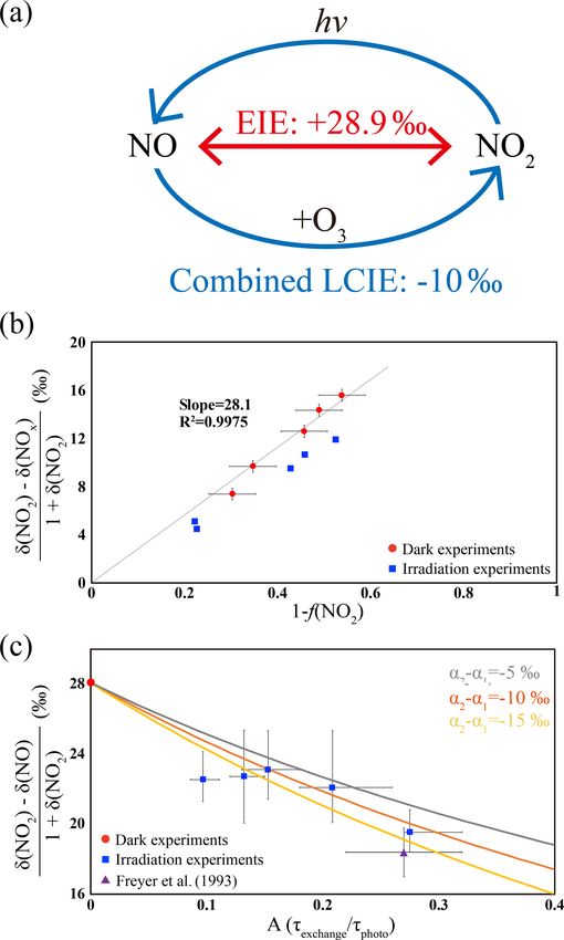
9806 J. Li et al.: Quantifying the nitrogen isotope effects of NOx photochemistry
position in ice and snow (Frey et al., 2009), may impact the
δ 15 N of NOy and atmospheric nitrate. The fractionation be-
tween NO and NO2 via isotope exchange has been suggested
to be the dominant factor in determining the δ 15 N of NO2
and ultimately atmospheric nitrate (Freyer, 1991; Freyer et
al., 1993; Savarino et al., 2013; Walters et al., 2016). How-
ever, isotopic fractionations occur in most, if not all, NOx
and NOy reactions, while most of these are still unknown
or, if calculated (Walters and Michalski, 2015), unverified
by experiments. Since the atmospheric chemistry of NOy
varies significantly in different environments (e.g., polluted
vs. pristine, night vs. day), the isotopic fractionations associ-
ated with NOy chemistry are also likely to vary in different
environments. These unknowns could potentially bias con-
clusions about NOx source apportionment reached when us-
ing nitrogen isotopes. Therefore, understanding the isotopic
fractionations between NO and NO2 during photochemical
cycling could improve our understanding of the relative role
of sources versus chemistry for controlling the δ 15 N varia-
tions in atmospheric NO2 and nitrate.
In general, there are three types of isotopic fractiona-
tion effects associated with NOx chemistry (Fig. 1a). The
first type is the equilibrium isotopic effect (EIE), i.e., iso-
tope exchange between two compounds without forming
new molecules (Urey, 1947; Bigeleisen and Mayer, 1947),
which for nitrogen isotopes in the NOx system is the
15 NO+14 NO ↔ 14 NO+15 NO exchange reaction (Begun
2 2
and Melton, 1956; Walters et al., 2016). The second type is
the kinetic isotopic effect (KIE) associated with difference
in isotopologue rate coefficients during unidirectional reac-
tions (Bigeleisen and Wolfsberg, 1957). In the NOx system
this KIE would manifest in the oxidation of NO into NO2 by
O3 /HO2 /RO2 . The third type is the photochemical isotope
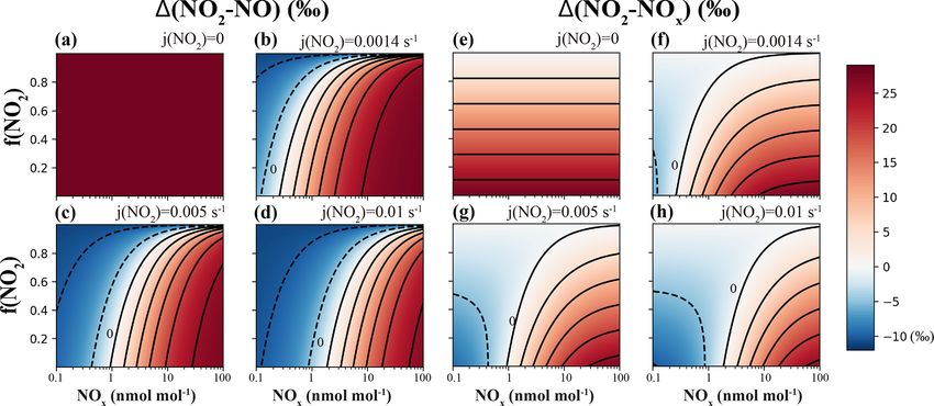
Figure 1. (a) A sketch of the isotopic fractionation processes be-
fractionation effect (PHIFE; Miller and Yung, 2000), which
tween NO and NO2 ; both fractionation factors are determined in
for NOx is the isotopic fractionation associated with NO2
this work. (b) Results from five dark experiments (red circles)
photolysis. All three fractionations could impact the δ 15 N yielded a line with slope of 28.1 ‰ and an α(NO2 –NO) value of
value of NO2 and consequently atmospheric nitrate, but the 1.0289, while the results from five UV irradiation experiments (blue
relative importance of each may vary. squares) showed a smaller slope. (c) Results from five UV irradia-
The limited number of studies on the EIE in the NOx cy- tion experiments (blue squares) and a previous field study (purple
cle have significant uncertainties. Discrepancies in the EIE triangle), comparing to the dark experiments (red circle). The three
for 15 NO+14 NO2 ↔ 14 NO+15 NO2 have been noted in sev- lines represent different (α2 − α1 ) values: the (α2 − α1 ) = −10 ‰
eral studies. Theoretical calculations predicted isotope frac- line showed the lowest RMSE to our experimental data as well as
tionation factors (α) ranging from 1.035 to 1.042 at room the previous field observations. The error bars in panels (b) and (c)
temperature (Begun and Fletcher, 1960; Monse et al., 1969; represented the combined uncertainties of NOx concentration mea-
surements and isotopic analysis.
Walters and Michalski, 2015) due to the different approx-
imations used to calculate harmonic frequencies in each
study. Likewise, two separate experiments measured differ-
ent room temperature fractionation factors of 1.028 ± 0.002 ent environment is uncertain because of possible wall effects
(Begun and Melton, 1956) and 1.0356 ± 0.0015 (Walters et and formation of higher oxides, notably N2 O4 and N2 O3 at
al., 2016). A concern in both experiments is that they were these high NOx concentrations.
conducted in small chambers with high NOx concentrations Even less research has examined the KIE and PHIFE oc-
(hundreds of micromoles per mole), significantly higher than curring during NOx cycling. The KIE of NO + O3 has been
typical ambient atmospheric NOx levels (usually less than theoretically calculated (Walters and Michalski, 2016) but
0.1 µmol mol−1 ). Whether the isotopic fractionation factors has not been experimentally verified. The NO2 PHIFE has
determined by these experiments are applicable in the ambi- not been experimentally determined or theoretically calcu-
Atmos. Chem. Phys., 20, 9805–9819, 2020 https://doi.org/10.5194/acp-20-9805-2020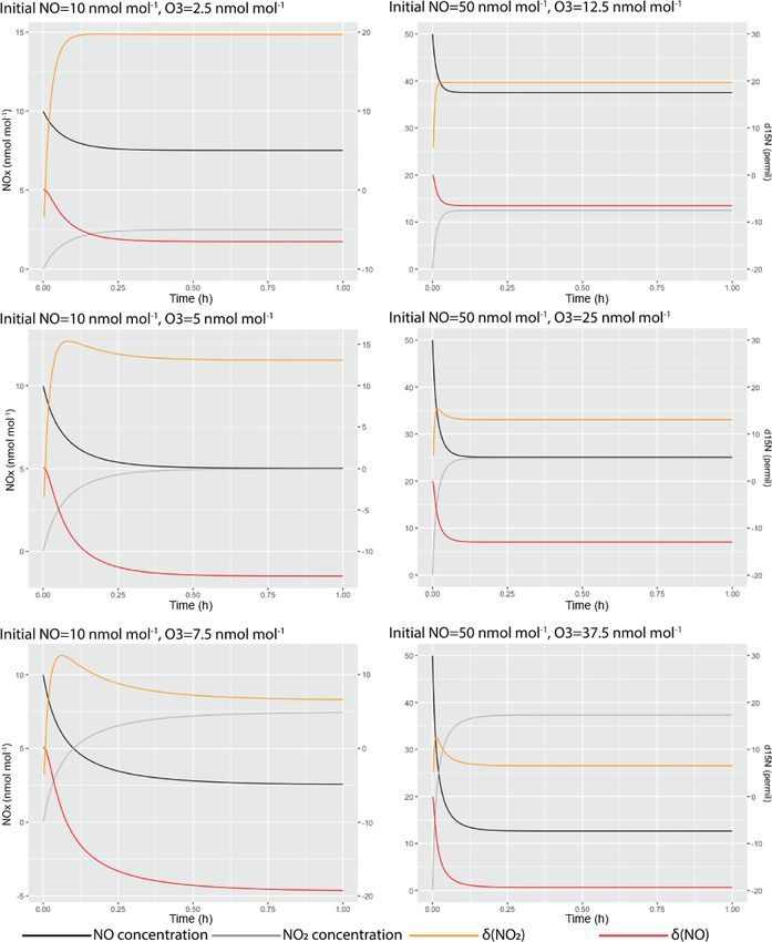
J. Li et al.: Quantifying the nitrogen isotope effects of NOx photochemistry                                               9807

lated. As a result, field observation studies often overlook      in NO2 concentrations was observed, showing that chamber
the effects of PHIFE and KIE. Freyer et al. (1993) mea-           wall loss was negligible.
sured NOx concentrations and the δ 15 N values of NO2 over           Three experiments were conducted to measure the δ 15 N
a 1-year period at Julich, Germany, and inferred a com-           value of the tank NO (i.e., the δ 15 N value of total NOx ).
bined NOx isotope fractionation factor (EIE+KIE+PHIFE)            In each of these experiments, a certain amount of O3 was
of 1.018±0.001. Freyer et al. (1993) suggested that the NOx       first injected into the chamber, then approximately the same
photochemical cycle (KIE and PHIFE) tends to diminish             amount of NO was injected into the chamber to ensure
the equilibrium isotopic fractionation (EIE) between NO and       100 % of the NOx was in the form of NO2 with little O3
NO2 . Even if this approach were valid, applying this single      (< 15 nmol mol−1 ) remaining in the chamber such that the
fractionation factor elsewhere, where NOx and O3 concentra-       O3 + NO2 reaction was negligible. The NO2 in the cham-
tions and actinic fluxes are different, would be tenuous given    ber was then collected and its δ 15 N value measured, which
that these factors may influence the relative importance of       equates to the δ 15 N value of the tank NO.
EIE, KIE and PHIFE (Hastings et al., 2004; Walters et al.,           Two sets of experiments were conducted to separately in-
2016). Therefore, to quantify the overall isotopic fractiona-     vestigate the EIE, KIE and PHIFE. The first set of exper-
tions between NO and NO2 at various tropospheric condi-           iments was conducted in the dark. In each of these dark
tions, it is crucial to know (1) isotopic fractionation factors   experiments, a range of NO and O3 ([O3 ] < [NO]) was in-
of EIE, KIE and PHIFE individually and (2) the relative im-       jected into the chamber to produce NO–NO2 mixtures with
portance of each factor under various conditions.                 [NO]/[NO2 ] ratios ranging from 0.43 to 1.17. The N isotopes
   In this work, we aim to quantify the nitrogen isotope frac-    of these mixtures were used to investigate the EIE between
tionation factors between NO and NO2 at photochemical             NO and NO2 . The second set of experiments was conducted
equilibrium. First, we measure the N isotope fractionations       under irradiation of UV lights (300–500 nm; see Appendix A
between NO and NO2 in an atmospheric simulation cham-             for irradiation spectrum). Under such conditions, NO, NO2
ber at atmospherically relevant NOx levels. Then, we provide      and O3 reached a photochemically steady state, which com-
mathematical solutions to assess the impact of NOx level and      bined the isotopic effects of EIE, KIE and PHIFE.
NO2 photolysis rate (j (NO2 )) on the relative importance of         In all experiments, the concentrations of NO, NO2 and O3
EIE, KIE and PHIFE. Subsequently we use the solutions and         were allowed to reach a steady state, and the product NO2
chamber measurements to calculate the isotopic fractionation      was collected from the chamber using a honeycomb denuder
factors of EIE, KIE and PHIFE. Lastly, using the calculated       tube. After the NO, NO2 and O3 concentrations reached a
fractionation factors and the equations, we model the NO–         steady state, well-mixed chamber air was drawn out through
NO2 isotopic fractionations at several sites to illustrate the    a 40 cm long Norprene thermoplastic tubing at 10 L min−1
behavior of δ 15 N values of NOx in the ambient environment.      and passed through a honeycomb denuder system (Chem-
                                                                  comb 3500, Thermo Scientific). Based on flow rate, the NO2
                                                                  residence time in the tubing was less than 0.5 s; thus in the
2   Methods                                                       light-on experiments where NO and O3 coexisted, the NO2
                                                                  produced inside the transfer tube through NO + O3 reac-
The experiments were conducted using a 10 m3 atmospheric          tions should be < 0.03 nmol mol−1 (using the upper limit of
simulation chamber at the National Center for Atmospheric         NO and O3 concentrations in our experiments). The hon-
Research (see descriptions in Appendix A and Zhang et al.,        eycomb denuder system consisted of two honeycomb de-
2018). A set of mass flow controllers was used to inject          nuder tubes connected in series. Each honeycomb denuder
NO and O3 into the chamber. NO was injected at 1 L min−1          tube is a glass cylinder 38 mm long and 47 mm in diame-
from an in-house NO/N2 cylinder (133.16 µmol mol−1 NO             ter and consists of 212 hexagonal tubes with inner diame-
in ultrapure N2 ), and O3 was generated by flowing zero air       ters of 2 mm. Before collecting samples, each denuder tube
through a flow tube equipped with a UV Pen-Ray lamp (UVP          was coated with a solution of 10 % KOH and 25 % guaiacol
LLC., CA) into the chamber at 5 L min−1 . NO and NO2              in methanol and then dried by flowing N2 gas through the
concentrations were monitored in real time by chemilumi-          denuder tube for 15 s (Williams and Grosjean, 1990; Wal-
nescence with a detection limit of 0.5 nmol mol−1 (model          ters et al., 2016). The NO2 reacted with the guaiacol coating
CLD 88Y, Eco Physics, MI) as were O3 concentrations us-           and was converted into NO−     2 that was retained on the de-
ing a UV absorption spectroscopy with a detection limit of        nuder tube wall (Williams and Grosjean, 1990). NO was in-
0.5 nmol mol−1 (model 49, Thermo Scientific, CO). In each         ert to the denuder tube coating: a control experiment sampled
experiment, the actual amounts of NO and O3 injected were         pure NO using the denuder tubes, which did not show any
calculated using measured NOx and O3 concentrations after         measurable NO−    2 . The NO2 collection efficiency of a single
a steady state was reached (usually within 1 h). The wall loss    honeycomb denuder tube was tested in another control ex-
rate of NO2 was tested by monitoring O3 (29 nmol mol−1 )          periment: air containing 66 nmol mol−1 of NO2 was drawn
and NOx (62 nmol mol−1 ) over a 4 h period. After the NO          out of the chamber through a denuder tube, and the NO2
and NO2 concentrations reached a steady state, no decrease        concentration at the exit of the tube holder was measured

https://doi.org/10.5194/acp-20-9805-2020                                           Atmos. Chem. Phys., 20, 9805–9819, 2020
9808 J. Li et al.: Quantifying the nitrogen isotope effects of NOx photochemistry
and found to be below the detection limit (< 1 nmol mol−1 ), tor (α(NO2 –NO)) is then calculated to be
suggesting that the collection efficiency was nearly 100 %
when [NO2 ] < 66 nmol mol−1 . Furthermore, when the de- [15 NO2 ][14 NO] R(NO2 )
α(NO2 –NO) = = , (1)
nuder system consisted of two denuder tubes in series, NO− 2 [14 NO2 ][15 NO] R(NO)
in the second denuder was below the detection limit, indi-
cating trivial NO2 breakthrough. Each NO2 collection lasted where R(NO, NO2 ) are the 15 N/14 N ratios of NO and NO2 .
for 0.5–3 h in order to collect enough NO− By definition, the δ 15 N(NO) is (R(NO)/R(reference) − 1) ×
2 for isotopic
analysis (at least 300 nmol). After collection, the NO− 1000 ‰, and δ 15 N(NO2 ) is (R(NO2 )/R(reference) − 1) ×
2 was
leached from each denuder tube by rinsing thoroughly with 1000 ‰, but hereafter, the δ 15 N values of NO, NO2 and NOx
10 mL deionized water into a clean polypropylene container are referred to as δ(NO), δ(NO2 ) and δ(NOx ), respectively.
and stored frozen until isotopic analysis. Isotopic analysis Equation (1) leads to
was conducted at the Purdue Stable Isotope Laboratory. For
each sample, approximately 50 nmol of the NO− δ (NO2 ) − δ (NO) = (α (NO2 –NO) − 1) (1 + δ(NO)). (2)
2 extract was
mixed with 2 M sodium azide solution in an acetic acid buffer
Using Eq. (2) and applying NOx isotopic mass bal-
in an airtight glass vial, then shaken overnight to completely
ance (δ(NOx ) = f (NO2 )δ(NO2 ) + (1 − f (NO2 ))δ(NO),
reduce all the NO− 2 to N2 O(g) (Casciotti and McIlvin, 2007; f (NO2 ) = [NO2 ]/([NO] + [NO2 ])) yields
McIlvin and Altabet, 2005). The product N2 O was directed
into a Thermo Scientific GasBench equipped with a cryotrap, δ (NO2 ) − δ (NOx ) α (NO2 –NO) − 1
then the δ 15 N of the N2 O was measured using a Delta-V iso- = (1 − f (NO2 )) . (3)
1 + (NO2 ) α (NO2 –NO)
tope ratio mass spectrometer (IRMS). Six coated denuder
tubes that did not get exposed to NO2 were also analyzed Here, δ(NOx ) equals the δ 15 N value of the cylinder NO, and
using the same chemical procedure, which did not show any f (NO2 ) is the molar fraction of NO2 with respect to total
measurable signal on the IRMS, suggesting that the blank NOx . Three experiments (Table 1) that measured δ(NOx )
from both the sampling process and the chemical conversion showed consistent δ(NOx ) values of −58.7 ± 0.8 ‰ (n = 3),
process was negligible. The overall analytical uncertainty for indicating that δ(NOx ) remained unchanged throughout the
δ 15 N analysis was 0.5 ‰ (1σ ) based on replicate analysis of experiments (as expected for isotope mass balance). Thus,
in-house NO− 2 standards. the δ(NOx ) can be treated as a constant in Eq. (3), and the
linear regression of (δ(NO2 ) − δ(NOx ))/(1 + δ(NO2 )) ver-
sus 1 − f (NO2 ) should have an intercept of 0 and a slope of
3 Results and discussions (α(NO2 –NO) − 1)/α(NO2 –NO).
The plot of (δ(NO2 ) − δ(NOx ))/(1 + δ(NO2 )) as a func-
3.1 Equilibrium isotopic fractionation between NO and
tion of 1 − f (NO2 ) values from five experiments yields an
NO2
α(NO2 –NO) value of 1.0289 ± 0.0019 at room temperature
The equilibrium isotope fractionation factor, α(NO2 –NO), is (Fig. 1b and Table 1). This fractionation factor is compa-
the 15 N enrichment in NO2 relative to NO and is expressed rable to previously measured values but with some differ-
as the ratio of rate constants k2 /k1 of two reactions: ences. Our result agrees well with the α(NO2 –NO) value of
1.028±0.002 obtained by Begun and Melton (1956) at room
15
NO2 +14 NO → 15 NO+14 NO2 , temperature. However, Walters et al. (2016) determined the
α(NO2 –NO) values of NO–NO2 exchange in a 1 L reaction
rate constant = k1 (R1)
vessel, which showed a slightly higher α(NO2 –NO) value
15 14 15 14
NO+ NO2 → NO2 + NO, of 1.035. This discrepancy might originate from rapid het-
rate constant = k2 = k1 α(NO2 –NO), (R2) erogeneous reactions on the wall of the reaction vessel at
high NOx concentrations and the small chamber size used
where k1 is the rate constant of the isotopic exchange, by Walters et al. (2016). They used a reaction vessel made
which was previously determined to be 8.14×10⁻¹⁴ cm3 s−1 of Pyrex, which is known to absorb water (Do Remus et al.,
(Sharma et al., 1970). The reaction time required for NO– 1983; Takei et al., 1997) and can react with NO2 , forming
NO2 to reach isotopic equilibrium was estimated using the HONO, HNO3 and other N compounds. Additionally, pre-
exchange rate constants in a simple kinetics box model vious studies have suggested that Pyrex walls enhance the
(BOXMOX; Knote et al., 2015). The model predicts that at formation rate of N2 O4 by over an order of magnitude (Bar-
typical NOx concentrations used during the chamber experi- ney and Finlayson-Pitts, 2000; Saliba et al., 2001), which at
ments (7.7–62.4 nmol mol−1 ), isotopic equilibrium would be isotopic equilibrium is enriched in 15 N compared to NO and
reached within 15 min (see Appendix B). Since the sam- NO2 (Walters and Michalski, 2015). Therefore, their mea-
ple collection usually started 1 h after NOx was well mixed sured α(NO2 –NO) might be slightly higher than the actual
in the chamber, there was sufficient time to reach full iso- α(NO2 –NO) value. In this work, the 10 m3 chamber has
tope equilibrium. The isotope equilibrium fractionation fac- a much smaller surface-to-volume ratio relative to Walters
Atmos. Chem. Phys., 20, 9805–9819, 2020 https://doi.org/10.5194/acp-20-9805-2020J. Li et al.: Quantifying the nitrogen isotope effects of NOx photochemistry 9809
Table 1. Experimental conditions; concentrations of NO, NO2 and O3 at a steady state; and measured δ(NO2 ) values.
Experiment Number NO conc. NO2 conc. O3 conc. δ(NO2 ) f (NO2 )
(nmol mol−1 ) (nmol mol−1 ) (nmol mol−1 ) (‰ )
Determining 1 0.0 17.8 13.4 −59.5 1.00
δ(NOx ) 2 0.0 61.3 0.5 −58.9 1.00
3 0.0 18.9 10.7 −58.0 1.00
Dark 1 16.0 36.8 0.0 −51.8 0.70
experiments 2 33.6 28.8 0.0 −43.9 0.46
3 6.7 12.6 0.0 −49.6 0.65
4 16.2 16.9 0.0 −45.1 0.51
5 20.4 24.2 0.0 −46.8 0.54
Irradiation 1 7.1 6.4 2.8 −47.5 0.47
experiments 2 4.5 5.3 4.5 −48.7 0.54
3 3.3 4.4 4.2 −49.8 0.57
4 2.5 8.5 10.7 −54.6 0.77
5 5.2 18.1 11.0 −54.0 0.78
et al. (2016), which minimizes wall effects, and the walls pounds (VOCs) in the chamber, so no RO2 was produced,
were made of Teflon, which minimizes NO2 surface reac- which excludes the NO + RO2 reaction. Likewise, the low
tivity, as evidenced by the NO2 wall loss control experi- water vapor content (relative humidity < 10 %) and the mi-
ment. Furthermore, the low NOx mixing ratios in our exper- nor flux of photons (< 310 nm) results in minimal OH pro-
iments minimized N2 O4 and N2 O3 formation. At NO and duction and hence little HO2 formation, and subsequently a
NO2 concentrations of 50 nmol mol−1 , the steady-state con- trivial amount of NO2 would be formed by NO + HO2 . Ap-
centrations of N2 O4 and N2 O3 were calculated to be 0.014 plying these limiting assumptions, the EIE between NO and
and 0.001 pmol mol−1 , respectively (Atkinson et al., 2004). NO2 (Reactions R1–R2) is only competing with the KIE (Re-
Therefore, we suggest that our measured α(NO2 –NO) value actions R3–R4) and the PHIFE in Reactions (R5)–(R6):
(1.0289 ± 0.0019) may better reflect the room temperature
14
(298 K) NO–NO2 EIE in the ambient environment. NO2 → 14 NO + O,
Unfortunately, the chamber temperature could not be con- rate constant = j (NO2 ) (R3)
trolled, so we were not able to investigate the temperature de- 15 15
pendence of the EIE. Hence, we speculate that the α(NO2 – NO2 → NO + O,
NO) follows a similar temperature dependence pattern cal- rate constant = j (NO2 )α1 (R4)
culated in Walters et al. (2016). Walters et al. (2016) sug- 14
NO + O3 → 14
NO2 + O2 ,
gested that the α(NO2 –NO) value would be 0.0047 higher
at 273 K and 0.002 lower at 310 K relative to room tem- rate constant = k5 (R5)
perature (298 K). Using this pattern and our experimentally 15 15
NO + O3 → NO2 + O2 ,
determined data, we suggest that the α(NO2 –NO) values at rate constant = k5 α2 , (R6)
273, 298 and 310 K are 1.0336±0.0019, 1.0289±0.0019 and
1.0269 ± 0.0019, respectively. This 0.0067 variation at least in which j (NO2 ) is the NO2 photolysis rate (1.4 × 10⁻³ s−1
partially contributes to the daily and seasonal variations in in these experiments), k5 is the rate constant for the NO + O3
δ 15 N values of NO2 and nitrate in some areas (e.g., polar reaction (1.73 × 10⁻¹⁴ cm3 s−1 ; Atkinson et al., 2004), and
regions with strong seasonal temperature variation). Thus, α1,2 are isotopic fractionation factors for the two reactions.
future investigations should be conducted to verify the EIE Previous studies (Freyer et al., 1993; Walters et al., 2016)
temperature dependence. have attempted to assess the competition between EIE (Reac-
tions R1–R2), KIE and PHIFE (Reactions R3–R6), but none
3.2 Kinetic isotopic fractionation of Leighton cycle of them quantified the relative importance of the two pro-
cesses, nor were α1 or α2 values experimentally determined.
The photochemical reactions of NOx will compete with the Here we provide the mathematical solution of EIE, KIE and
isotope exchange fractionations between NO and NO2 . The PHIFE to illustrate how Reactions (R1)–(R6) affect the iso-
NO–NO2 photochemical cycle in the chamber was controlled topic fractionations between NO and NO2 .
by the Leighton cycle: NO2 photolysis and the NO + O3 re-
action. This is because there were no volatile organic com-
https://doi.org/10.5194/acp-20-9805-2020 Atmos. Chem. Phys., 20, 9805–9819, 20209810 J. Li et al.: Quantifying the nitrogen isotope effects of NOx photochemistry
First, the NO2 lifetime with respect to isotopic exchange and 0.9929 at 310 K. The total variation in α2 values from
with NO (τexchange ) and photolysis (τphoto ) was determined: 273 to 310 K is only 1.4 ‰, significantly smaller than our
experimental uncertainty (±5 ‰). The α1 value was calcu-
1 lated using a zero-point energy (ZPE) shift model (Miller and
τexchange = (4)
k1 [NO] Yung, 2000) to calculate the isotopic fractionation of NO2 by
1 photolysis. Briefly, this model assumes both isotopologues
τphoto = . (5)
j (NO2 ) have the same quantum yield function, and the PHIFE was
only caused by the differences in the 15 NO2 and 14 NO2 ab-
We then define an A factor: sorption cross section as a function of wavelength; thus α1
values do not vary by temperature. The 15 NO2 absorption
( τ
exchange
τphoto when j (NO2 ) 6 = 0
A= (6) cross section was calculated by shifting the 14 NO2 absorp-
0 when j (NO2 ) = 0.
tion cross section by the 15 NO2 zero-point energy (Michal-
Using Reactions (R1)–(R6) and Eqs. (1)–(6), we solved ski et al., 2004). When the ZPE shift model was used with
steady-state δ(NO2 ) and δ(NO) values (see calculations in the irradiation spectrum of the chamber lights, the resulting
Appendix C). Our calculations show that the δ(NO2 )–δ(NO) α1 value was 1.0023. Therefore, the theoretically predicted
and δ(NO2 )–δ(NOx ) values at a steady state can be ex- α2 −α1 value should be −0.0090, i.e., −9.0±0.7 ‰ when the
pressed as functions of α1 , α2 , α(NO2 –NO) and A: temperature ranges from 273 to 310 K. This result shows ex-
cellent agreement with our experimentally determined room
(α2 − α1 ) A + (α (NO2 –NO) − 1) temperature α2 − α1 value of −10 ± 5 ‰ .
δ (NO2 ) − δ (NO)=
α2 A + α (NO2 –NO) This model was then used to evaluate the variations in
(1 + δ (NO2 )) α1 under different lighting conditions. The tropospheric ul-
(α2 − α1 ) A + (α (NO2 –NO) − 1) traviolet and visible (TUV) radiation model (TUV5.3.2;
≈ Madronich and Flocke, 1999) was used to calculate the so-
A+1
(1 + δ (NO2 )) (7) lar wavelength spectrum at three different conditions: early
morning or late afternoon (solar zenith angle = 85◦ ), mid-
(α2 − α1 ) A + (α (NO2 –NO) − 1)
δ (NO2 ) − δ (NOx )= morning or afternoon (solar zenith angle = 45◦ ), and 12:00
α2 A + α (NO2 –NO)
local time (LT; solar zenith angle = 0◦ ). These spectra were
(1 + δ (NO2 )) (1 − f (NO2 )) used in the ZPE shift model to calculate the α1 values, which
(α2 − α1 ) A + (α (NO2 –NO) − 1) are 1.0025, 1.0028 and 1.0029 at solar zenith angles of 85,
≈
A+1 45 and 0◦ , respectively. These values, along with the pre-
(1 + δ (NO2 )) (1 − f (NO2 )). (8) dicted α1 value in the chamber, showed a total span of 0.6 ‰
(1.0026 ± 0.0003), which is again significantly smaller than
Equation (7) shows the isotopic fractionation between NO our measured uncertainty. Therefore, we suggest that our ex-
and NO2 ; δ(NO2 )–δ(NO) is mainly determined by A; the perimentally determined LCIE factor (−10 ± 5 ‰) can be
EIE factor (α(NO2 –NO) − 1) and the (α2 − α1 ) factor as- used in most tropospheric solar irradiation spectra.
suming 1 + δ(NO2 ) is close to 1. This (α2 − α1 ) repre- The equations can also be applied in tropospheric envi-
sents a combination of KIE and PHIFE, suggesting that ronments to calculate the combined isotopic fractionations
they act together as one factor; therefore, we name the of EIE and LCIE for NO and NO2 . First, the NO2 sink re-
(α2 − α1 ) factor the Leighton cycle isotopic effect (LCIE). actions (mainly NO2 + OH in the daytime) are at least 2–3
Using measured δ(NO2 ) and δ(NOx ) values, A values (Ta- orders of magnitude slower than the Leighton cycle and the
ble 1), and the previously determined
α(NO2 –NO) value, we NO–NO2 isotope exchange reactions (Walters et al., 2016);
δ(NO2 )−δ(NOx ) δ(NO2 )−δ(NO)
plot (1+δ(NO2 ))(1−f (NO2 )) equals (1+δ(NO2 )) against the therefore their effects on the δ(NO2 ) should be minor. Sec-
A value and use Eqs. (7) and (8) to estimate the (α2 − α1 ) ond, although the conversion of NO into NO2 in the ambi-
value (Fig. 1c). The plot shows that the best fit for the LCIE ent environment is also controlled by NO + RO2 and HO2
factor is (−10 ± 5) ‰ (root mean square error, RMSE, was in addition to NO + O3 (e.g., King et al., 2001), Eq. (7) still
lowest when α2 − α1 = −10 ‰). The uncertainties in the showed good agreement with field observations in previous
LCIE factor are relatively higher than that of the EIE factor, studies. Freyer et al. (1993) determined the annual average
mainly because of the accumulated analytical uncertainties daytime δ(NO2 )–δ(NO) at Julich, Germany, along with av-
at low NOx and O3 concentrations and low A values (0.10– erage daytime NO concentration (9 nmol mol−1 , similar to
0.28) due to the relatively low j (NO2 ) value (1.4×10⁻³ s−1 ) our experimental conditions) to be +18.03 ± 0.98 ‰. Us-
under the chamber irradiation conditions. ing Eq. (7), assuming the daytime average j (NO2 ) value
This LCIE factor determined in our experiments is in good throughout the year was (5.0 ± 1.0) × 10−3 , and a calculated
agreement with theoretical calculations. Walters and Michal- A value from measured NOx concentration ranged from 0.22
ski (2016) previously used an ab initio approach to determine to 0.33, the average NO–NO2 fractionation factor was calcu-
an α2 value of 0.9933 at room temperature, 0.9943 at 237 K lated to be +19.8 ± 1.4 ‰ (Fig. 1c), in excellent agreement
Atmos. Chem. Phys., 20, 9805–9819, 2020 https://doi.org/10.5194/acp-20-9805-2020J. Li et al.: Quantifying the nitrogen isotope effects of NOx photochemistry 9811
with the measurements in the present study. This agreement NO–NO2 isotopic fractionations in two ways: (1) changes
suggests that the NO + RO2 /HO2 reactions might have sim- in the j (NO2 ) value would change the photolysis intensity
ilar fractionation factors as NO + O3 . Therefore, we suggest and therefore the τphoto value; (2) in addition, changes in
that Eqs. (7) and (8) can be used to estimate the isotopic frac- the j (NO2 ) value would also alter the steady-state NO con-
tionations between NO and NO2 in the troposphere. centration, therefore changing the τexchange (Fig. 2c). The
combined effect of these two factors on the A value varies
3.3 Calculating nitrogen isotopic fractionations of along with the atmospheric conditions and thus needs to be
NO–NO2 carefully calculated using NOx concentration data and atmo-
spheric chemistry models.
First, Eq. (7) was used to calculate the 1(NO2 –NO) = We then calculated the differences in δ 15 N values between
δ(NO2 )–δ(NO) at a wide range of NOx concentrations NO2 and total NOx , e.g., 1(NO2 –NOx ) = δ(NO2 )–δ(NOx )
and f (NO2 ) and j (NO2 ) values (Fig. 2a–d), assuming 1 + in Fig. 2e–h. Since 1(NO2 –NOx ) are connected through
δ(NO2 ) ≈ 1. j (NO2 ) values of 0 s−1 (Fig. 2a), 1.4×10⁻³ s−1 the observed δ 15 N of NO2 (or nitrate) to the δ 15 N of NOx
(Fig. 2b), 5 × 10⁻³ s−1 (Fig. 2c) and 1 × 10⁻² s−1 (Fig. 2d) sources, this term might be useful in field studies (e.g., Chang
were selected to represent nighttime, dawn (as well as the et al., 2018; Zong et al., 2017). The calculated 1(NO2 –NOx )
laboratory conditions of our experiments), daytime average values (Fig. 2e–h) also showed an LCIE-dominated regime
and 12:00 LT, respectively. Each panel represented a fixed at low [NOx ] and an EIE-dominated regime at high [NOx ].
j (NO2 ) value, and the 1(NO2 –NO) values were calculated The 1(NO2 –NOx ) values were dampened by the 1−f (NO2 )
as a function of the A value, which was derived from NOx factor comparing to 1(NO2 –NO), as shown in Eqs. (3) and
concentration and f (NO2 ). The A values have a large span, (8): 1(NO2 –NOx ) = 1(NO2 –NO) (1 − f (NO2 )). At high
from 0 to 500, depending on the j (NO2 ) value and the NO f (NO2 ) values (> 0.8), the differences between δ(NO2 ) and
concentration. When A = 0 (j (NO2 ) = 0) and f (NO2 ) < 1 δ(NOx ) were less than 5 ‰; thus the measured δ(NO2 ) val-
(meaning NO and NO2 coexist and [O3 ] = 0), Eqs. (7) and ues were similar to δ(NOx ), although the isotopic fractiona-
(8) become Eqs. (2) and (3), showing that the EIE was the tion between NO and NO2 could be noteworthy. Some ambi-
sole factor; the 1(NO2 –NO) values were solely controlled ent environments with significant NO emissions or high NO2
by EIE, which has a constant value of +28.9 ‰ at 298 K photolysis rates usually have f (NO2 ) values between 0.4 and
(Fig. 2a). When j (NO2 ) > 0, the calculated 1(NO2 –NO) 0.8 (Mazzeo et al., 2005; Vicars et al., 2013). In this scenario,
values showed a wide range from −10.0 ‰ (controlled by the 1(NO2 –NOx ) values in Fig. 2f–h showed wide ranges
LCIE factor: α2 − α1 = −10 ‰) to +28.9 ‰ (controlled by of −4.8 ‰ to +15.6 ‰, −6.0 ‰ to +15.0 ‰ and −6.3 ‰ to
EIE factor: α(NO2 –NO) − 1 = +28.9 ‰). Figure 2b–d dis- +14.2 ‰ at j (NO2 ) = 1.4×10⁻³ , 5×10⁻³ and 1×10⁻² s−1 ,
play the transition from an LCIE-dominated regime to an respectively. These significant differences again highlighted
EIE-dominated regime. The LCIE-dominated regime is char- the importance of both LCIE and EIE (Eqs. 7 and 8) in cal-
acterized by low [NOx ] (< 50 pmol mol−1 ), representing re- culating the 1(NO2 –NOx ). In the following discussion, we
mote ocean areas and polar regions (Beine et al., 2002; Cus- assume that (1) the α1 value remains constant (see discussion
tard et al., 2015). At this range the A value can be greater above), (2) the NO+RO2 /HO2 reactions have the same frac-
than 200; thus Eq. (7) can be simplified as 1(NO2 –NO) = tionation factors (α2 ) as NO+O3 , and (3) both EIE and LCIE
α2 − α1 , suggesting that the LCIE almost exclusively con- do not display significant temperature dependence. We then
trols the NO–NO2 isotopic fractionation. The 1(NO2 –NO) use Eqs. (7) and (8) and this laboratory-determined LCIE fac-
values of these regions are predicted to be < 0 ‰ during most tor (−10 ‰) to calculate the nitrogen isotopic fractionation
times of the day and < −5 ‰ at 12:00 LT. On the other hand, between NO and NO2 at various tropospheric atmospheric
the EIE-dominated regime was characterized by high [NOx ] conditions.
(> 20 nmol mol−1 ) and low f (NO2 ) (< 0.6), representative
of regions with intensive NO emissions, e.g., near roadside
or stack plumes (Clapp and Jenkin, 2001; Kimbrough et al., 4 Implications
2017). In this case, the τexchange are relatively short (10–50 s)
compared to the τphoto (approximately 100 s at 12:00 LT and The daily variations in 1(NO2 –NOx ) values at two road-
1000 s at dawn); therefore the A values are small (0.01–0.5). side NOx monitoring sites were predicted to demonstrate
The EIE factor in this regime thus is much more important the effects of NOx concentrations to the NO–NO2 isotopic
than the LCIE factor, resulting in high 1(NO2 –NO) values fractionations. Hourly NO and NO2 concentrations were ac-
(> 20 ‰). Between the two regimes, both EIE and LCIE are quired from a roadside site at Anaheim, CA (https://www.
competitive, and therefore it is necessary to use Eq. (7) to arb.ca.gov, last access: 9 August 2019), and an urban site at
quantify the 1(NO2 –NO) values. Evansville, IN (http://idem.tx.sutron.com, last access: 9 Au-
Figure 2 also implies that changes in the j (NO2 ) value can gust 2019), on 25 July 2018. The hourly j (NO2 ) values out-
cause the diurnal variations in 1(NO2 –NO) values. Chang- put from the TUV model (Madronich and Flocke, 1999) at
ing j (NO2 ) would affect the value of A and consequently the these locations were used to calculate the daily variations
https://doi.org/10.5194/acp-20-9805-2020 Atmos. Chem. Phys., 20, 9805–9819, 20209812 J. Li et al.: Quantifying the nitrogen isotope effects of NOx photochemistry Figure 2. Calculating isotopic fractionation values between NO–NO2 (1(NO2 –NO); a–d) and NOx –NO2 (1(NO2 –NOx ); e–h) at various j (NO2 ), NOx level and f (NO2 ) using Eqs. (7) and (8). Each panel represents a fixed j (NO2 ) value (on the upper-right side of each panel), and the fractionation values are shown by color. Lines are contours with the same fractionation values at an interval of 5 ‰; the contour line representing 0 ‰ was marked in each panel except for panels (a) and (e). in 1(NO2 –NOx ) values (Fig. 3a, b) by applying Eq. (8) amount of NO was produced by direct NO emission and NO2 and assuming 1 + δ(NO2 ) ≈ 1. Hourly NOx concentrations photolysis, but the f (NO2 ) was still high (0.73 ± 0.08). Our were 12–51 nmol mol−1 at Anaheim and 9–38 nmol mol−1 calculation suggested that the daytime 1(NO2 –NOx ) values at Evansville, and the f (NO2 ) values at both sites did not should be only +1.3±3.2 ‰, with a lowest value of −1.3 ‰. show significant daily variations (0.45 ± 0.07 at Anaheim These 1(NO2 –NOx ) values were similar to the observed and and 0.65 ± 0.08 at Evansville), likely because the NOx con- modeled summer daytime δ(NO2 ) values in West Lafayette, centrations were controlled by the high NO emissions from IN (Walters et al., 2018), which suggest that the average day- the road (Gao, 2007). The calculated 1(NO2 –NOx ) values time 1(NO2 –NOx ) values at NOx = 3.9 ± 1.2 nmol mol−1 using Eq. (8) showed significant diurnal variations. During should range from +0.1 ‰ to +2.4 ‰. In this regime, we the nighttime, the isotopic fractionations were solely con- suggest that the 1(NO2 –NOx ) values were generally small trolled by the EIE; the predicted 1(NO2 –NOx ) values were due to the significant contribution of LCIE and high f (NO2 ). +14.5±2.0 ‰ and +8.7±2.1 ‰ at Anaheim and Evansville, The LCIE should be the dominant factor controlling the respectively. During the daytime, the existence of LCIE low- NO–NO2 isotopic fractionation in remote regions, resulting ered the predicted 1(NO2 –NOx ) values to +9.8 ± 1.7 ‰ at in a completely different diurnal pattern of 1(NO2 –NOx ) Anaheim and +3.1 ± 1.5 ‰ at Evansville, while the f (NO2 ) compared with the urban–suburban area. Direct hourly mea- values at both sites remained similar. The lowest 1(NO2 – surements of NOx at remote sites are rare; thus we used a NOx ) values for both sites (+7.0 ‰ and +1.7 ‰) occurred total NOx concentration of 50 pmol mol−1 and a daily O3 around 12:00 LT, when the NOx photolysis was the most in- concentration of 20 nmol mol−1 at Summit, Greenland (Dibb tense. In contrast, if one neglects the LCIE factor in the day- et al., 2002; Hastings et al., 2004; Honrath et al., 1999; Yang time, the 1(NO2 –NOx ) values would be +12.9 ± 1.5 ‰ and et al., 2002) and assumed 1 + δ(NO2 ) ≈ 1 and that the con- +10.0 ± 1.6 ‰, respectively, an overestimation of 3.1 ‰ and version of NO to NO2 was completely controlled by O3 to 6.9 ‰. These discrepancies suggested that the LCIE played calculate the NO/NO2 ratios. Here the isotopes of NOx were an important role in the NO–NO2 isotopic fractionations, and almost exclusively controlled by the LCIE due to the high A neglecting it could bias the NOx source apportionment using values (> 110). The 1(NO2 –NOx ) values displayed a clear δ 15 N of NO2 or nitrate. diurnal pattern (Fig. 3d), with a maximum value of −0.3 ‰ The role of LCIE was more important in less polluted in the “nighttime” (solar zenith angle > 85◦ ) and a mini- sites. The 1(NO2 –NOx ) values were calculated for a subur- mum value of −5.0 ‰ during midday. This suggests that ban site near San Diego, CA, USA, again using the hourly the isotopic fractionations between NO and NO2 were al- NOx concentrations (https://www.arb.ca.gov; Fig. 3c) and most completely controlled by LCIE in remote regions when j (NO2 ) values calculated from the TUV model. NOx con- NOx concentrations were < 0.1 nmol mol−1 . However, since centrations at this site varied from 1 to 9 nmol mol−1 , assum- the isotopic fractionation factors of nitrate formation reac- ing 1 + δ(NO2 ) ≈ 1. During the nighttime, NOx was in the tions (NO2 +OH, NO3 +HC, N2 O5 +H2 O) are still unknown, form of NO2 (f (NO2 = 1) because O3 concentrations were more studies are needed to fully explain the daily and sea- higher than NOx ; thus the δ(NO2 ) values should be identi- sonal variations in δ(NO− 3 ) in remote regions. cal to δ(NOx ) (1(NO2 –NOx ) = 0). In the daytime a certain Atmos. Chem. Phys., 20, 9805–9819, 2020 https://doi.org/10.5194/acp-20-9805-2020
J. Li et al.: Quantifying the nitrogen isotope effects of NOx photochemistry                                                        9813

Figure 3. NOx concentrations and calculated 1(NO2 –NOx ) values at four sites. Stacked bars show the NO and NO2 concentrations extracted
from monitoring sites (a–c) or calculated using a 0-D box model (d); the red lines are 1(NO2 –NOx ) values at each site. Note that the NOx
concentration (left y axis in panel d) is different from the rest.

   Nevertheless, our results have a few limitations. First, cur-       tribute to the seasonality of isotopic fractionations between
rently there are very few field observations that can be used to       NOx and NOy molecules.
evaluate our model; therefore, future field observations that
measure the δ 15 N values of ambient NO and NO2 should be
carried out to test our model. Second, more work, includ-              5   Conclusions
ing theoretical and experimental studies, is needed to inves-
                                                                       The effect of NOx photochemistry on the nitrogen isotopic
tigate the isotope fractionation factors occurring during the
                                                                       fractionations between NO and NO2 was investigated. We
conversion from NOx to NOy and nitrate: in the NOy cy-
                                                                       first measured the isotopic fractionations between NO and
cle, EIE (isotopic exchange between NO2 , NO3 and N2 O5 ),
                                                                       NO2 and provided mathematical solutions to assess the im-
KIE (formation of NO3 , N2 O5 and nitrate) and PHIFE (pho-
                                                                       pact of NOx level and NO2 photolysis rate (j (NO2 )) on the
tolysis of NO3 , N2 O5 , HONO and sometimes nitrate) may
                                                                       relative importance of EIE and LCIE. The EIE and LCIE
also exist and be relevant for the δ 15 N of HNO3 and HONO.
                                                                       isotope fractionation factors at room temperature were de-
In particular, the N isotope fractionation occurring during
                                                                       termined to be 1.0289 ± 0.0019 and 0.990 ± 0.005, respec-
the NO2 + OH → HNO3 reaction needs investigation. Such
                                                                       tively. These calculations and measurements can be used to
studies could help us to model the isotopic fractionation be-
                                                                       determine the steady-state 1(NO2 –NO) and 1(NO2 –NOx )
tween NOx emission and nitrate and eventually enable us to
                                                                       values at room temperature. Subsequently we applied our
analyze the δ 15 N value of NOx emission by measuring the
                                                                       equations to polluted, clean and remote sites to model the
δ 15 N values of nitrate aerosols and nitrate in wet depositions.
                                                                       daily variations in 1(NO2 –NOx ) values. We found that the
Third, our discussion only focuses on the reactive nitrogen
                                                                       1(NO2 –NOx ) values could vary from over +20 ‰ to less
chemistry in the troposphere; however, the nitrogen chem-
                                                                       than −5 ‰ depending on the environment: in general, the
istry in the stratosphere is drastically different from the tro-
                                                                       role of LCIE becomes more important at low NOx concentra-
pospheric chemistry; thus future studies are also needed to
                                                                       tions, which tend to decrease the 1(NO2 –NOx ) values. Our
investigate the isotopic fractionations in the stratospheric ni-
                                                                       work provided a mathematical approach to quantify the ni-
trogen chemistry. Last, the temperature dependence of both
                                                                       trogen isotopic fractionations between NO and NO2 that can
EIE and LCIE needs to be carefully investigated because of
                                                                       be applied to many tropospheric environments, which could
the wide range of temperature in both the troposphere and
                                                                       help interpret the measured δ 15 N values of NO2 and nitrate
stratosphere. Changes in temperature could alter the isotopic
                                                                       in field observation studies.
fractionation factors of both EIE and LCIE as well as con-

https://doi.org/10.5194/acp-20-9805-2020                                                 Atmos. Chem. Phys., 20, 9805–9819, 2020
9814 J. Li et al.: Quantifying the nitrogen isotope effects of NOx photochemistry
Appendix A: Chamber descriptions Appendix B: Box model assessing the time needed for
NO–NO2 to reach isotopic equilibrium
The chamber is a 10 m3 Teflon bag equipped with several
standard instruments including a temperature and humidity The time needed to reach NO–NO2 isotopic equilibrium
probe, NOx monitor and O3 monitor. A total of 128 wall- during light-off experiments was assessed using a 0-D box
mounted blacklight tubes surrounded the chamber to mimic model. This box model contains only two reactions:
tropospheric photochemistry, and the photolysis rate of NO2
15
(j (NO2 )) when all lights are on has been previously deter- NO2 +14 NO → 15 NO+14 NO2
mined to be 1.4 × 10⁻³ s−1 , similar to a j (NO2 ) coefficient k = 8.14000 × 10⁻¹⁴ cm3 s−1 (BR1)
at an 81◦ solar zenith angle. The irradiation spectrum of the
15
black lights is shown in Fig. A1. The chamber was kept at NO+14 NO2 → 15 NO2 +14 NO
room temperature and 1 atm. Before each experiment, the k 0 = 8.37525 × 10⁻¹⁴ cm3 s−1 , (BR2)
chamber was flushed with zero air at 40 L min−1 for at least
12 h to ensure the background NOx , O3 and other trace gases where k and k 0 are rate constants of the reactions. The dif-
were below the detection limit. ferences in rate constants were calculated by assuming an
α(NO2 –NO) value of 1.0289. Six simulations were con-
ducted at various initial NO (with δ 15 N = 0 ‰) and O3 levels
that were similar to our experiment. Then the δ 15 N values of
NO and NO2 during the simulation were calculated from the
model and are shown in Fig. B1, suggesting that in our ex-
perimental condition, all systems should reach isotopic equi-
librium within 1 h.
Figure A1. Spectral actinic flux versus wavelengths of the UV light
source used in our experiments.
Atmos. Chem. Phys., 20, 9805–9819, 2020 https://doi.org/10.5194/acp-20-9805-2020J. Li et al.: Quantifying the nitrogen isotope effects of NOx photochemistry 9815 Figure B1. Simulated NO–NO2 isotopic equilibrium process in the chamber at various NO and O3 concentrations. https://doi.org/10.5194/acp-20-9805-2020 Atmos. Chem. Phys., 20, 9805–9819, 2020
9816                                                J. Li et al.: Quantifying the nitrogen isotope effects of NOx photochemistry

Appendix C: Deriving Eqs. (7) and (8)                                 Divide both sides by k1 [NO][NO2 ]:

When the system (Reactions R1–R6) reaches a steady state,                      k5 α2 [O3 ]
                                                                      RNO2     k1 [NO2 ] + α(NO2 –NO)
we have                                                                    =            jNO2 α1
                                                                                                      .                                (C10)
                                                                      RNO
                                                                                         k1 [NO] + 1
d[15 NO2 ]/dt = 0.                                           (C1)
                                                                                                  k5 [O3 ]          jNO2
                                                                      Rearrange and substitute   k1 [NO2 ]   and   k1 [NO]   with A:
Therefore, using Reactions (R1)–(R6)
                                                                      RNO2   α2 A + α(NO2 –NO)
k1 [15 NO2 ][14 NO] + j (NO2 )α1 [15 NO2 ] =                               =                                                           (C11)
                                                                      RNO          α1 A + 1
       15                               15     14
k5 α2 [ NO][O3 ] + k1 α(NO2 –NO)[ NO][ NO2 ].                (C2)     RNO          α1 A + 1
                                                                           =                                                           (C12)
                          14 NO        14 NO                          RNO2   α2 A + α(NO2 –NO)
From here we refer to      2 and      as NO2 and NO for
                                                                      RNO        (α1 − α2 ) A − (α(NO2 –NO) − 1)
convenience. Rearranging the above equation, we get                        −1 =                                  .                     (C13)
                                                                      RNO2              α1 A + α(NO2 –NO)
[15 NO2 ] k5 α2 [O3 ] + k1 α(NO2 –NO)[NO2 ]
         =                                  .                (C3)     Thus,
 [15 NO]          jNO2 α1 + k1 [NO]
                                                                      δ(NO2 )−δ(NO) =
Meanwhile, since the Leighton cycle reaction still holds for
the majority of isotopes (NO and NO2 ), we have                                (α2 − α1 ) A + (α(NO2 –NO) − 1)
                                                                                      α1 A + α(NO2 –NO)
jNO2 [NO2 ] = k5 [NO][O3 ].                                  (C4)              (1 + δ(NO2 )).                                          (C14)
Thus,                                                                 Then, using mass balance
[NO2 ] k5 × [O3 ]
      =           .                                          (C5)     δ(NO2 )f (NO2 ) + δ(NO)(1 − f (NO2 )) = δ(NOx )                  (C15)
 [NO]    jNO2
                                                                      we can derive Eq. (8):
From the text, when jNO2 > 0, we defined A =
τexchange /τphoto = jNO2 /(k1 × [NO]). Using the above                δ(NO2 )−δ(NOx ) =
equations, we know
                                                                               (α2 − α1 ) × A + α(NO2 –NO) − 1
jNO2    k5 [O3 ]                                                                      α1 A + α(NO2 –NO)
      =          = Ak1                                       (C6)
[NO]    [NO2 ]                                                                 (1 + δ(NO2 )) (1 − f (NO2 )) .                          (C16)
 jNO2       k5 [O3 ]
        =            = A.                                    (C7)
k1 [NO] k1 [NO2 ]
Next, to calculate δ(NO2 )–δ(NO), we use the definition of
delta notation:
δ(NO2 )–δ(NO) = RNO2 /RSD − RNO /RSD
                    = (RNO2 /RNO − 1)(1 + δ(NO))             (C8)
            15
RNO2      NO2 [NO]
     = 15
RNO       NO [NO2 ]
            k5 α2 [O3 ] [NO] + k1 α(NO2 –NO) [NO2 ] [NO]
        =                                                .   (C9)
                    jNO2 α1 [NO2 ] + k1 [NO] [NO2 ]

Atmos. Chem. Phys., 20, 9805–9819, 2020                                               https://doi.org/10.5194/acp-20-9805-2020
J. Li et al.: Quantifying the nitrogen isotope effects of NOx photochemistry 9817
Data availability. Data acquired from this study were Bigeleisen, J. and Wolfsberg, M.: Theoretical and experimental as-
deposited at Open Sciences Framework (Li, 2019; pects of isotope effects in chemical kinetics, Adv. Chem. Phys.,
https://doi.org/10.17605/OSF.IO/JW8HU). 1, 15–76, https://doi.org/10.1002/9780470143476.ch2, 1957.
Casciotti, K. L. and McIlvin, M. R.: Isotopic analyses of nitrate
and nitrite from reference mixtures and application to East-
Author contributions. JL and GM designed the experiments, XZ ern Tropical North Pacific waters, Mar. Chem., 107, 184–201,
and JL conducted the experiments. XZ, GM, JO and GT helped JL https://doi.org/10.1016/j.marchem.2007.06.021, 2007.
in interpreting the results. The manuscript was written by JL, and all Chang, Y., Zhang, Y., Tian, C., Zhang, S., Ma, X., Cao, F., Liu,
the authors have contributed during the revision of the manuscript. X., Zhang, W., Kuhn, T., and Lehmann, M. F.: Nitrogen iso-
tope fractionation during gas-to-particle conversion of NOx to
NO− 3 in the atmosphere – implications for isotope-based NOx
Competing interests. The authors declare that they have no conflict source apportionment, Atmos. Chem. Phys., 18, 11647–11661,
of interest. https://doi.org/10.5194/acp-18-11647-2018, 2018.
Clapp, L. J. and Jenkin, M. E.: Analysis of the relationship
between ambient levels of O3 , NO2 and NO as a func-
tion of NOx in the UK, Atmos. Environ., 35, 6391–6405,
Acknowledgements. We thank the NCAR’s Advanced Study Pro-
https://doi.org/10.1016/S1352-2310(01)00378-8, 2001.
gram for providing support to Jianghanyang Li. The National Cen-
Custard, K. D., Thompson, C. R., Pratt, K. A., Shepson, P. B., Liao,
ter for Atmospheric Research is operated by the University Corpo-
J., Huey, L. G., Orlando, J. J., Weinheimer, A. J., Apel, E., Hall,
ration for Atmospheric Research under the sponsorship of the Na-
S. R., Flocke, F., Mauldin, L., Hornbrook, R. S., Pöhler, D., Gen-
tional Science Foundation.
eral, S., Zielcke, J., Simpson, W. R., Platt, U., Fried, A., Weib-
ring, P., Sive, B. C., Ullmann, K., Cantrell, C., Knapp, D. J.,
and Montzka, D. D.: The NOx dependence of bromine chem-
Financial support. This research has been supported by the Na- istry in the Arctic atmospheric boundary layer, Atmos. Chem.
tional Science Foundation. Phys., 15, 10799–10809, https://doi.org/10.5194/acp-15-10799-
2015, 2015.
Dibb, J. E., Arsenault, M., Peterson, M. C., and Honrath, R. E.:
Review statement. This paper was edited by Jan Kaiser and re- Fast nitrogen oxide photochemistry in Summit, Greenland snow,
viewed by Matthew Johnson and one anonymous referee. Atmos. Environ., 36, 2501–2511, https://doi.org/10.1016/S1352-
2310(02)00130-9, 2002.
Do Remus, R. H., Mehrotra, Y., Lanford, W. A., and Bur-
man, C.: Reaction of water with glass: influence of a
transformed surface layer, J. Mater. Sci., 18, 612–622,
References https://doi.org/10.1007/BF00560651, 1983.
Elliott, E. M., Kendall, C., Boyer, E. W., Burns, D. A., Lear,
Atkinson, R., Baulch, D. L., Cox, R. A., Crowley, J. N., Hamp- G. G., Golden, H. E., Harlin, K., Bytnerowicz, A., Butler,
son, R. F., Hynes, R. G., Jenkin, M. E., Rossi, M. J., and T. J., and Glatz, R.: Dual nitrate isotopes in dry deposition:
Troe, J.: Evaluated kinetic and photochemical data for atmo- Utility for partitioning NOx source contributions to landscape
spheric chemistry: Volume I – gas phase reactions of Ox , HOx , nitrogen deposition, J. Geophys. Res.-Biogeo., 114, G04020,
NOx and SOx species, Atmos. Chem. Phys., 4, 1461–1738, https://doi.org/10.1029/2008JG000889, 2009.
https://doi.org/10.5194/acp-4-1461-2004, 2004. Felix, J. D. and Elliott, E. M.: Isotopic composition of pas-
Barney, W. S. and Finlayson-Pitts, B. J.: Enhancement of N2 O4 on sively collected nitrogen dioxide emissions: Vehicle, soil and
porous glass at room temperature: A key intermediate in the het- livestock source signatures, Atmos. Environ., 92, 359–366,
erogeneous hydrolysis of NO2 ?, J. Phys. Chem. A, 104, 171– https://doi.org/10.1016/j.atmosenv.2014.04.005, 2014.
175, https://doi.org/10.1021/jp993169b, 2000. Felix, J. D., Elliott, E. M., and Shaw, S. L.: Nitrogen iso-
Begun, G. M. and Fletcher, W. H.: Partition function ratios for topic composition of coal-fired power plant NOx : influ-
molecules containing nitrogen isotopes, J. Chem. Phys., 33, ence of emission controls and implications for global emis-
1083–1085, https://doi.org/10.1063/1.1731338, 1960. sion inventories, Environ. Sci. Technol., 46, 3528–3535,
Begun, G. M. and Melton, C. E.: Nitrogen isotopic fraction- https://doi.org/10.1021/es203355v, 2012.
ation between NO and NO2 and mass discrimination in Frey, M. M., Savarino, J., Morin, S., Erbland, J., and Martins, J.
mass analysis of NO2 , J. Chem. Phys., 25, 1292–1293, M. F.: Photolysis imprint in the nitrate stable isotope signal in
https://doi.org/10.1063/1.1743215, 1956. snow and atmosphere of East Antarctica and implications for
Beine, H. J., Honrath, R. E., Dominé, F., Simpson, W. R., and reactive nitrogen cycling, Atmos. Chem. Phys., 9, 8681–8696,
Fuentes, J. D.: NOx during background and ozone depletion pe- https://doi.org/10.5194/acp-9-8681-2009, 2009.
riods at Alert:Fluxes above the snow surface, J. Geophys. Res.- Freyer, H. D.: Seasonal variation of 15 N/14 N ratios
Atmos., 107, ACH-7, https://doi.org/10.1029/2002JD002082, in atmospheric nitrate species, Tellus B, 43, 30–44,
2002. https://doi.org/10.1034/j.1600-0889.1991.00003.x, 1991.
Bigeleisen, J. and Mayer, M. G.: Calculation of equilibrium con- Freyer, H. D., Kley, D., Volz-Thomas, A., and Kobel, K.: On the
stants for isotopic exchange reactions, J. Chem. Phys., 15, 261– interaction of isotopic exchange processes with photochemical
267, https://doi.org/10.1063/1.1746492, 1947.
https://doi.org/10.5194/acp-20-9805-2020 Atmos. Chem. Phys., 20, 9805–9819, 2020You can also read