Effect of leading-edge curvature actuation on flapping fin performance
←
→
Page content transcription
If your browser does not render page correctly, please read the page content below

J. Fluid Mech. (2021), vol. 921, A22, doi:10.1017/jfm.2021.469
Downloaded from https://www.cambridge.org/core. MIT Libraries, on 09 Jul 2021 at 18:36:23, subject to the Cambridge Core terms of use, available at https://www.cambridge.org/core/terms. https://doi.org/10.1017/jfm.2021.469
Effect of leading-edge curvature actuation on
flapping fin performance
David Fernández-Gutiérrez1 and Wim M. van Rees1, †
1 Department
of Mechanical Engineering, Massachusetts Institute of Technology, Cambridge,
MA 02139, USA
(Received 13 November 2020; revised 26 March 2021; accepted 23 May 2021)
Ray-finned fish are able to adapt the curvature of their fins through musculature
at the base of the fin. In this work we numerically investigate the effects of such
leading-edge curvature actuation on the hydrodynamic performance of a heaving and
pitching fin. We present a geometric and numerical framework for constructing the
shape of ray-membrane-type fins with imposed leading-edge curvatures, under the
constraint of membrane inextensibility. This algorithm is coupled with a three-dimensional
Navier–Stokes solver, enabling us to assess the hydrodynamic performance of such fins.
To determine the space of possible shapes, we present a simple model for leading-edge
curvature actuation through two coefficients that determine chordwise and spanwise
curvature, respectively. We systematically vary these two parameters through regimes that
mimic both passive elastic deformations and active actuation against the hydrodynamic
loading, and compute thrust and power coefficients, as well as hydrodynamic efficiency.
Our results demonstrate that both thrust and efficiency are predominantly affected
by chordwise curvature, with some small additional benefits of spanwise curvature
on efficiency. The main improvements in performance are explained by the altered
trailing-edge kinematics arising from leading-edge curvature actuation, which can largely
be reproduced by a rigid fin whose trailing-edge kinematics follow that of the curving
fin. Changes in fin camber, for fixed trailing-edge kinematics, mostly benefit efficiency.
Based on our results, we discuss the use of leading-edge curvature actuation as a robust
and versatile way to improve flapping fin performance.
Key words: swimming/flying, propulsion, wakes
1. Introduction
The potential of biologically inspired flapping fin propulsion for practical applications lies
in its predicted ability to provide high efficiency at a range of speeds, high manoeuvrability
† Email address for correspondence: wvanrees@mit.edu
© The Author(s), 2021. Published by Cambridge University Press 921 A22-1
Downloaded from https://www.cambridge.org/core. MIT Libraries, on 09 Jul 2021 at 18:36:23, subject to the Cambridge Core terms of use, available at https://www.cambridge.org/core/terms. https://doi.org/10.1017/jfm.2021.469
D. Fernández-Gutiérrez and W.M. van Rees
and a concealed profile. This has spurred a tremendous scientific effort over the last
few decades (Triantafyllou, Triantafyllou & Yue 2000; Smits 2019) to understand and
design bio-inspired propulsion techniques. A significant development within this design
landscape is driven by recent developments in additive manufacturing and smart structures,
so that robotic swimmers increasingly incorporate soft, flexible materials (Chu et al. 2012;
Christianson et al. 2018; Katzschmann et al. 2018). This leads to increasingly complex
systems, whose behaviour is characterized both by passive elastic deformation of the
structure as well as actuation degrees of freedom that can induce actively controlled shape
changes. Consequently, there is a need to understand to what extent such dynamic shape
changes affect hydrodynamic performance of flapping fin propulsion.
Passively deforming elastic surfaces have been studied extensively, as their input
parameters and performance can be easily tested and controlled in experimental and
numerical settings (Katz & Weihs 1978; Prempraneerach, Hover & Triantafyllou 2003).
Using two-dimensional (2-D) flat plates, Dewey et al. (2013) and Quinn, Lauder & Smits
(2014, 2015) show how the largest thrust is attained when a combination of heave and
pitch of the leading edge is imposed so resonance with structural natural frequencies
occurs. This conclusion is shared by Tytell et al. (2016) using numerical simulations of a
2-D anguilliform swimmer modelled using a fully coupled biomechanical–hydrodynamic
model. In three dimensions, Liu & Bose (1997) performed potential flow simulations
of a heaving and pitching fin whale fluke, imposing spanwise deformations across the
entire chord. Comparing with a rigid fin, they found spanwise deformations akin to
elastic deformation to decrease efficiency and thrust, and spanwise deformations that
mimic active deformations to increase thrust without affecting efficiency. Specifically
for caudal fins, Zhu (2007) and Zhu & Shoele (2008) performed potential flow coupled
fluid–structure interaction simulations. They conclude that, for underwater swimming,
increasing chordwise flexibility slightly increases efficiency and decreases thrust,
whereas increasing spanwise flexibility decreases trust without significantly affecting
efficiency.
The above works, except for Liu & Bose (1997), rely on a structural model of the
fin to model passive, elastic deformations due to the hydrodynamic loading. Natural
rayed fish fins, however, are composed of collagen membranes supported by bony rays
that can be actively curved through a set of muscles at the base of each ray (Lauder
& Drucker 2004; Alben, Madden & Lauder 2007). As a result, dynamic curvature
changes of real fish fins can consist of passive bending due to hydrodynamic loading,
as well as active actuation of the individual rays against the flow (Fish & Lauder
2006). Biological observations show that this musculature is active even during steady
swimming (Flammang & Lauder 2008), and that these combined effects lead to complex
three-dimensional (3-D) fin shapes (Bainbridge 1963; Lauder & Madden 2007; Lauder
2015) consisting of both chordwise (along rays) and spanwise (across rays) curvature
components. This was quantified in Lauder et al. (2005) and Bozkurttas et al. (2009),
who used a proper orthogonal decomposition to break down the fin motion into various
modes, observed also experimentally in real fish by Flammang & Lauder (2008, 2009).
Their results show how a discrete number of modes capture properly the most common
fin motion gaits. Using a robotic rayed caudal fin model, Lauder et al. (2007), Tangorra,
Esposito & Lauder (2009) and Esposito et al. (2012) analysed the contribution to the thrust
production for each of the individual deformation modes. They identified active cupping as
the mode that produces the largest amount of thrust, where the spanwise shape variations
are parabolic in nature, in phase with the pitch, and with the top and bottom rays leading
the motion.
921 A22-2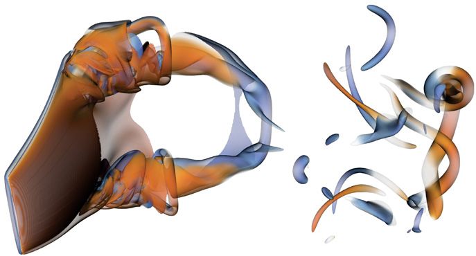
Downloaded from https://www.cambridge.org/core. MIT Libraries, on 09 Jul 2021 at 18:36:23, subject to the Cambridge Core terms of use, available at https://www.cambridge.org/core/terms. https://doi.org/10.1017/jfm.2021.469
Effect of curvature actuation on flapping fin performance
The above body of literature provides a picture that passive elastic deformations of
flapping fins can improve their efficiency and thrust production, although finding the best
structural design for a given hydrodynamic condition can be challenging. For spanwise
elastic deformations the hydrodynamic trends and structural design criteria have not yet
been systematically investigated. Further, there is an indication that actively curving
fins against the hydrodynamic loading can improve hydrodynamic performance, but this
requires further investigation.
Our current work is motivated by the wish to further understand the role of both
passive and active curvature changes on the hydrodynamic performance of flapping fin
propulsion. However, as opposed to the studies above, we do not explicitly consider
any specific elastic model of the fin. Instead, we parametrize the dynamic chordwise
and spanwise curvature variations of the fin geometry, and directly explore the effect
of imposed curvature variations on hydrodynamic performance. This enables us to side
step the fluid–structure interaction problem, and avoid making any assumptions about
materials, elastic properties and actuation techniques. Instead, our approach aims to
identify hydrodynamically beneficial curvature variations of the fin, and understand the
underlying flow mechanisms. In a future step, this information can then be used as a
target state for a fluid–structure interaction design study, aided by the capability of modern
actuation mechanisms for shape-changing structures (Boley et al. 2019).
In the following we detail the proposed mathematical representation of the fin geometry
in § 2.1, showing its capability to reproduce typical swimming modes observed in nature.
The 3-D Navier–Stokes solver used and its integration with the fin-shape generation
algorithm is described next in § 2.2. The particular problem definition of a deforming
fin subject to heave and pitch solid-body velocities, and the numerical set-up adopted
to simulate it, are then explained in § 3. Simulation results from the parametric analysis
of chordwise and spanwise curvature effects are presented in § 4, discussing in detail the
impact of each curvature type in §§ 5.1 and 5.2. Finally, we present our concluding remarks
in § 6.
2. Methodology
2.1. Description of fin shape
Our description and parametrization of the fin shape builds on our earlier work
(Fernández-Gutiérrez & van Rees 2020), with minor changes to the chordwise curvature
coefficient definition and non-dimensionalization of the curvature description. For clarity
and completeness we will therefore describe here the complete shape definition and its
derivation.
2.1.1. Geometric model
We represent any fin geometry by a parametric 3-D mid-surface definition combined with
a thickness distribution over it. Starting with the mid-surface, we introduce parameters
(u, v) where u ∈ [0, 1] and v ∈ [−1, 1]. The undeformed mid-surface is defined as
r 0 (u, v) = r LE (v) + u c(v) cos(β(v))x̂ + sin(β(v))ẑ , (2.1)
where
r LE (v) = xLE (v)x̂ + v(H/2)ẑ, (2.2)
is the leading-edge (LE) position vector and xLE (v) is the profile of the leading edge, as
shown in figure 1. Further, β(v) is the angle of the rays along the chordwise direction,
921 A22-3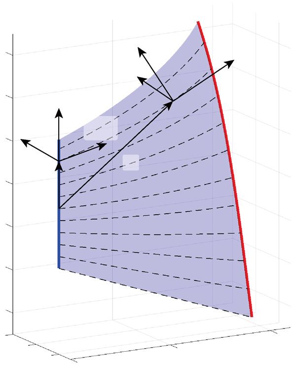
Downloaded from https://www.cambridge.org/core. MIT Libraries, on 09 Jul 2021 at 18:36:23, subject to the Cambridge Core terms of use, available at https://www.cambridge.org/core/terms. https://doi.org/10.1017/jfm.2021.469
D. Fernández-Gutiérrez and W.M. van Rees
z
(a) (b)
0.6 b̂ tˆ
x0 n̂
z0 0.4 b̂LE
β
x n̂LE tˆLE
H 0.2
A r
z 0 rLE
c A
–0.2
–0.4
C
–0.6
y A-A
LE h TE 0.4 1.0
0.2 0.5
u 0 0
y x
u=0 u=1
Figure 1. Notation and conventions for the geometric representation of the fin (a), and the local coordinate
system (b).
c(v) is the length of the chord as measured along a ray and H the height of the fin at the
leading edge (figure 1). The mapping and leading-edge position vector are defined such
that, in R3 , the ẑ-axis corresponds to the axis of rotation of the fin. With the mid-surface
defined, the description of the volumetric fin can be completed by the thickness function,
h(u, v), providing the distance between the outer fin surfaces along the normal of the fin’s
mid-surface. Throughout this work, we use the fin overall chord C as length scale, defined
as
C = max(r 0 · x̂) − min(r 0 · x̂). (2.3)
u,v u,v
To describe the deformed configuration of the mid-surface, we establish a Darboux
frame along the rays, as shown in figure 1(b). The frame is characterized by the tangent
unit vector along the rays, t̂, the normal unit vector to the mid-surface, n̂, and the bi-normal
unit vector b̂ = t̂ × n̂. Note that our vectors b̂ and n̂ are rotated compared with the normal
and binormal vectors arising using a Frenet framing of a space curve, due to the fact that,
here, n̂ corresponds to the mid-surface normal vector. Using the Darboux framing, we can
then define three non-dimensional curvatures corresponding to the directions of the local
coordinate system, defined as
⎫ ⎫
dt̂ ⎪
⎪ dn̂ db̂ ⎪
= +κ n̂ + κ b̂⎪
n g
⎪ κ =
t · b̂ = − · n̂⎪ ⎪
du ⎪
⎪ du du ⎪ ⎪
⎪
⎪
⎬ ⎪
⎬
dn̂ d t̂ db̂
= −κ t̂ + κ b̂
n t ↔ κ =
g · b̂ = − · t̂ ⎪ , (2.4)
du ⎪
⎪ du du ⎪
⎪
⎪ ⎪
⎪
⎪
⎪ ⎪
db̂ ⎪
⎭ dt̂ dn̂ ⎪ ⎪
= −κ t̂ − κ n̂
g t
κ =
n · n̂ = − · t̂ ⎭
du du du
where the curvatures are non-dimensional; the dimensionalized forms can be found when
multiplying with the local chord c(v). More precisely, the values of κ t , κ g and κ n ,
respectively, correspond to the geodesic torsion, geodesic curvature and normal curvature
of the constant-v curve on the mid-surface.
921 A22-4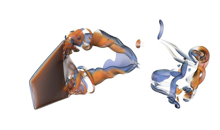
Downloaded from https://www.cambridge.org/core. MIT Libraries, on 09 Jul 2021 at 18:36:23, subject to the Cambridge Core terms of use, available at https://www.cambridge.org/core/terms. https://doi.org/10.1017/jfm.2021.469
Effect of curvature actuation on flapping fin performance
For the deformed configuration, we can then write the position of the mid-surface as
u
r(u, v) = r LE (v) + c(v) t̂(u∗ , v) du∗ , (2.5)
0
with r LE (v) defined as above, and u∗ an integration variable. We can in turn express t̂ in
terms of the curvatures from (2.4) as
u
t̂(u, v) = t̂LE (v) + κ n n̂ + κ g b̂ (u∗ , v) du∗ , (2.6)
0
where t̂LE (v) = cos(β(v))x̂ + sin(β(v))ẑ is the tangent unit vector at the undeformed LE.
The problem of finding the deformed mid-surface is then reduced to finding the functional
form of the three curvatures, or, equivalently, the basis (t̂, n̂, b̂) along each ray. Note that
when κ n = κ g = 0, we recover the flat configuration described in (2.1).
Mechanically, fish can actuate the rays at the LE to balance the hydrodynamic loading,
acting as control mechanism of κ n for each ray (Alben et al. 2007). Thus, κ n becomes a
controllable degree of freedom, allowing us to consider it as a known, user-defined input
whose specific form will be discussed further in § 3.2.
To find corresponding expressions for κ g and κ t , we use two assumptions. First, we
treat the membrane connecting the rays as inextensible based on its material properties
(Alben et al. 2007; Nguyen et al. 2017) so that ∂r/∂v = ∂r 0 /∂v. Second, we assume
that the membrane remains smooth, which discretely implies that the mid-surface normals
as obtained from integrating the Darboux frame along each ray are consistent with the
mid-surface normals as obtained from differentiating the position vector across rays, as
further explained in the next section.
Lastly, to obtain the volumetric shape of the deformed fin, we neglect the effect of
transverse normal and shear strains, similar to the Kirchhoff–Love assumptions in plate
and shell theory, so that the thickness function remains unchanged in the deformed
configuration.
2.1.2. Discrete representation and solution algorithm for the fin geometry
The exact solution to the mid-surface shape formulation described in § 2.1.1 is difficult to
find, so we propose here an iterative solution technique that maintains the discrete error in
satisfying the aforementioned constraints below a user-specified threshold.
We start by discretizing the mid-surface into a structured mesh with Nv rays in the
spanwise direction (indexed by i), each of which is represented through a set of Nu
equidistant nodes (indexed by j). Throughout, we assume a known functional form of κ n ,
g
and impose zero curvature at the tips (κi,Nu = κi,N
t
u
= 0) and symmetric κ t across the ic th
central element (ic = Nv /2),
0 Nv odd
κitc ,j /cic = . (2.7)
−κitc +1,j /cic +1 Nv even
g
We then assume initial values for the remaining values of κi,j and κi,j
t , and determine
the location of the ray nodes by discretely integrating the Darboux frame along each
ray, according to (2.4)–(2.6). Using a finite-difference approximation of the derivatives,
and noting that the resulting vector after applying the transformation needs to be
921 A22-5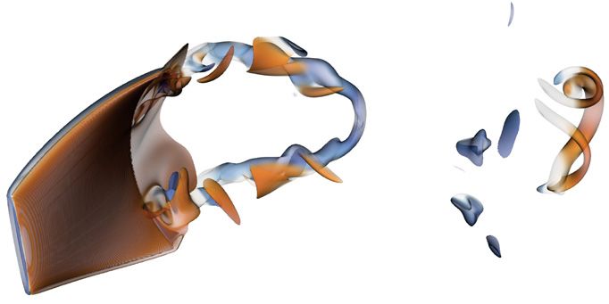
Downloaded from https://www.cambridge.org/core. MIT Libraries, on 09 Jul 2021 at 18:36:23, subject to the Cambridge Core terms of use, available at https://www.cambridge.org/core/terms. https://doi.org/10.1017/jfm.2021.469
D. Fernández-Gutiérrez and W.M. van Rees
re-normalized, this leads to a marching algorithm for the ith ray
⎡ g ⎤
0 −κi,j n −κi,j
K i,j = ⎣ κi,j
n −κi,jt ⎦
0 , (2.8)
g
κi,j κi,j t 0
∗ ∗ ∗ K i,j+1 + K i,j
t n b i,j+1 = t̂ n̂ b̂ I+ u , (2.9)
i,j 2
∗ ∗ ∗
t n b
t̂ n̂ b̂ = , (2.10)
i,j+1 t∗ n∗ b∗ i,j+1
t̂i,j + t̂i,j+1
r i,j+1 = r i,j + ci u, (2.11)
t̂i,j + t̂i,j+1
where I is the identity matrix and u = 1/(Nu − 1). For each ray, we use as initial values
the known LE position r i,1 and direction vectors [t̂, n̂, b̂]i,1 from the rigid-body kinematics.
Given the above procedure to compute the Darboux frame and position vector for
each ray, we can then update our initial guesses for κ g and κ t using a Newton–Raphson
algorithm. The goal of the algorithm is to minimize deviation from the inextensibility and
smoothness constraints, quantified by the signed error metrics Eldist and Elsmth , respectively:
⎧
⎪
⎪ r i+1,j − r i,j
⎪
⎪ − 1 i < ic : l = i + (j − 2)(Nv − 1),
⎪
⎨ di,j
Eldist = r i,j − r i−1,j (2.12)
⎪
⎪ − 1 i > ic : l = (i − 1) + (j − 2)(Nv − 1),
⎪
⎪ di−1,j
⎪
⎩
r i+1,j − r i−1,j
Elsmth = · n̂i,j l = i + (j − 2)Nv + (Nv − 1)(Nu − 1), (2.13)
r i+1,j − r i−1,j
where l is a global index to identify each unknown curvature, di,j the spanwise distance
between adjacent nodes in the undeformed configuration computed analytically from
(2.1) and (r i+1,j − r i−1,j ) the numerical approximation to the spanwise surface tangent
direction, which should be orthogonal to the surface normal vector n̂i,j .
We numerically differentiate these error metrics with respect to the unknown curvature
variables to determine the Jacobian of the system
⎡ ⎤
Eldist Eldist
⎢ κ g κmt ⎥ g g i < ic : m = i + (j − 1)(Nv − 1),
⎢ m ⎥ κm ≡ κi,j
J l,m ≈ ⎢ ⎥, i > ic : m = (i − 1) + (j − 1)(Nv − 1),
⎣ E smth E smth ⎦
l
g
l κ t ≡ κt
m i,j m = i + (j − 1)Nv + (Nv − 1)(Nu − 1).
κm κmt
(2.14a,b)
In each Newton–Raphson step we then invert the Jacobian matrix using a lower-upper
(LU) decomposition with partial pivoting to update the curvature values
g (k+1) g (k) dist (k)
κm κm (k) −1 El
= − J l,m , (2.15)
κmt κmt Elsmth
where k denotes the Newton–Raphson iteration. Given the new curvature values
κ g,(k+1) and κ t,(k+1) , we can again evaluate (2.8)–(2.11) to compute the corresponding
921 A22-6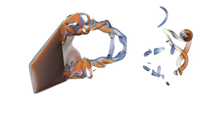
Downloaded from https://www.cambridge.org/core. MIT Libraries, on 09 Jul 2021 at 18:36:23, subject to the Cambridge Core terms of use, available at https://www.cambridge.org/core/terms. https://doi.org/10.1017/jfm.2021.469
Effect of curvature actuation on flapping fin performance
new Darboux frame and position vectors, and evaluate the associated error metrics
(2.12)–(2.13). If they are below a given threshold, |Eldist | < dist and |Elsmth | < smth ∀l,
the solution has been found and we stop. Otherwise, we start a new iteration by computing
the Jacobian matrix associated with the new ray configuration.
2.1.3. Interpolation to reduce computational cost
We can significantly improve the algorithm’s performance by solving for the values of κ t
and κ g on a coarser mesh, with Nr Nv rays and Ns Nu nodes along them, and use
interpolation to determine the intermediate values in the finer mesh taking advantage of
the smooth nature of the mid-surface.
We first construct a quadratic approximation to determine the chordwise derivatives of
κ t and κ g at each coarse grid node using three-point stencils with values at the node and its
t , κ g are determined between each pair
closest neighbours. Then, the interpolated values κi,j i,j
of nodes using a cubic interpolation using the curvatures and its derivatives at the nodes.
Using the interpolated curvatures along each ray, we can determine the fine-grid node
locations along each ray following (2.8)–(2.11). Then, we can obtain the fine-grid node
locations between rays following a similar interpolation procedure, now in the spanwise
direction, determining the derivative values using a quadratic fit and then interpolating
the node coordinates r i,j with a cubic spline. Note that, under this approach, the spanwise
position derivatives are computed explicitly for each node and therefore are continuous
across nodes.
With this adjustment, we still follow the iterative algorithm described in § 2.1.2,
substituting (i, j) → ( p, q) where p ∈ [1, Nr ] and q ∈ [1, Ns ]. In addition, we can use the
fine-grid interpolated nodes to compute the distance between nodes for Eldist , as well as the
spanwise surface tangent direction for Elsmth .
2.2. Three-dimensional Navier–Stokes solver
We use in this work the remeshed vortex method with a penalization technique (Gazzola
et al. 2011), which solves the 3-D viscous incompressible Navier–Stokes equations in
vorticity–velocity form
∂ω
+ (u · ∇)ω = (ω · ∇)u + ν∇ 2 ω + λ∇ × [χ(us − u)] , (2.16)
∂t
where ω = ∇ × u is the vorticity vector, ν the kinematic viscosity, and u is the fluid
velocity vector. The last term on the right-hand side is responsible for enforcing the
solid-body boundary conditions, with χ the characteristic function representing the body
(χ = 1 inside the body, χ = 0 outside and smoothly transitioning between those values at
the interface), us the imposed velocity inside the body and λ 1 the penalization factor
that dynamically forces the flow inside the body to follow the imposed body motion. As
explained in Gazzola et al. (2011), we solve the velocity from the vorticity by inverting
a Poisson’s equation with free-space boundary conditions, enabling the use of a compact
domain. This framework has been validated extensively in the past for simulations and
optimizations related to self-propelled 2-D and 3-D swimmers (Gazzola et al. 2011;
Gazzola, Van Rees & Koumoutsakos 2012; van Rees, Gazzola & Koumoutsakos 2013,
2015). In the context of this work, we also verified our method in appendix A in the
supplementary material available at https://doi.org/10.1017/jfm.2021.469 for flapping fin
propulsion specifically.
921 A22-7
Downloaded from https://www.cambridge.org/core. MIT Libraries, on 09 Jul 2021 at 18:36:23, subject to the Cambridge Core terms of use, available at https://www.cambridge.org/core/terms. https://doi.org/10.1017/jfm.2021.469
D. Fernández-Gutiérrez and W.M. van Rees
To integrate our model, we can decompose the body velocity field at any point r
inside the body as us (r, t) = uT (t) + uR (r, t) + udef (r, t), where uT (t) is the translational
velocity, uR (r, t) = θ̇(t) × r is the rigid-body rotational velocity (note that the fin pitches
around the z-axis, so the origin of the position vector r is always at the centre of rotation)
and udef (r, t) is the deformation velocity field arising from a time-varying curvature
distribution. In this work, uT (t) and θ̇(t) are imposed through the heave and pitch
kinematics of the fin, and χ (r, t) and udef (r, t) are determined from the geometric model
characterizing the fin shape described in § 2.1.
As in Bernier et al. (2019), we compute the overall hydrodynamic force and moment
acting on the body from the projection and penalization components, such that
F proj F penal
D
F = ∇ · σ dV = ρu dV + ρλχ (u − uS ) dV, (2.17)
Ωb Dt Vb Ωb
M proj M penal
D
M= r × (∇ · σ ) dV = r × (ρu) dV + r × [ρλ (u − uS )] dV, (2.18)
Ωb Dt Vb Ωb
where Ωb and Vb are the control and material volume of the solid body and σ is the
stress tensor. We further identify the horizontal component opposite to the incident flow
as thrust, and the transverse component in the direction of heave as lift,
T = −F · x̂, (2.19)
L = F · ŷ. (2.20)
Following a similar approach, we can compute the power required to overcome the
hydrodynamic loads and actuate the fin. Starting from the general definition (Winter 1987)
applied to a control volume coinciding with the body
P=− ∇ · (σ u) dV = − [(∇ · σ ) · u + ∇u : σ ] dV, (2.21)
Ωb Ωb
we can use the incompressible Newtonian stress tensor σ = −pI + μ(∇u + ∇uT ), where
p is the fluid pressure and T the transpose operator, to express the power as
D ρ
P=− μ∇u : ∇u + ∇u dV −T
u · u dV − λχ (u − uS ) · u dV.
Ωb Dt Vb 2 Ωb
(2.22)
3. Problem definition
In this section we will first explain our choice of flow regime and fin details, determined
by Reynolds and Strouhal number, the fin geometry and the rigid-body fin kinematics. We
will then explain our parametrization choices for the fin curvature through κ n . Finally, we
will discuss the numerical settings and performance metrics used to generate the results.
3.1. Flow regime and fin details
We model the fin shape as a simple trapezoidal planform pitching around the leading
edge, to simplify the large variety of fin shapes observed in nature. As discussed more
921 A22-8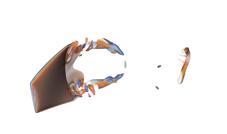
Downloaded from https://www.cambridge.org/core. MIT Libraries, on 09 Jul 2021 at 18:36:23, subject to the Cambridge Core terms of use, available at https://www.cambridge.org/core/terms. https://doi.org/10.1017/jfm.2021.469
Effect of curvature actuation on flapping fin performance
in depth in our previous work (Fernández-Gutiérrez & van Rees 2020), we choose H =
0.6C as leading-edge height and 1.35C as trailing-edge height inspired by the caudal fin
of a bluegill sunfish as a representative ray-finned fish. The fin moves with rigid-body
kinematics consisting of the following harmonic heaving and pitching motion:
y(t) = Ay sin(2πft), (3.1)
θ(t) = Aθ sin(2πft + ϕθ ), (3.2)
where f is the flapping frequency, Ay the heaving amplitude, Aθ the pitching amplitude
and ϕθ the phase angle between heave and pitch. The rigid-body components of the body
velocity us are then imposed as
uT (t) = ẏ(t)ŷ, (3.3)
uR (r, t) = θ̇(t)ẑ × r. (3.4)
The free parameters are chosen based on a review of existing studies in this realm.
Specifically, we set Ãy = Ay /C = 0.4, consistent with the suggestion of Triantafyllou et al.
(2000) of amplitudes of heave motion comparable to the chord lengths; we use Aθ = 30◦ ,
following the biological observations shown by Hu et al. (2016); and we choose ϕθ =
−90◦ , as suggested by Read, Hover & Triantafyllou (2003) for optimum efficiency.
The flow regime, characterized by the Reynolds number Re = U∞ C/ν, is limited by
the computational requirements of the solver. In this work we set it to Re = 1500, which
is lower than most adult fish but representative of smaller and early stage fishes. Based
on existing literature (Wu et al. 2020), we expect this Reynolds number to provide results
that are representative for flapping fins in the range 102 Re 104 . Lastly, the flapping
frequency is non-dimensionalized through the Strouhal number St = 2fAy /U∞ , where U∞
is the free-stream velocity magnitude. We fix the Strouhal number St = 0.3, consistent
with experimental observations of real fish and theoretical scaling laws at this Reynolds
number (Triantafyllou et al. 2000; Gazzola, Argentina & Mahadevan 2014a; Floryan, Van
Buren & Smits 2018). At the end of this work, we briefly mention the effect of increasing
the Strouhal number to St = 0.6, as an exploration of our results to propulsion with higher
thrust coefficients (appendix E.1 in the supplementary material).
3.2. Curvature parametrization
Although the algorithm presented in § 2.1.2 is general, we choose here a simple
parametrization of κ n that enables us to investigate a representative range of curvature
variations. First, we set the normal curvature to a constant along each ray, so that
κ n (u, v, t) = κ0n (v, t), which mimics the type of leading-edge control demonstrated in
real fish (Alben et al. 2007). Second, we define the leading-edge curvature as a linear
combination of uniform and parabolic curvature profiles across the span of the fin. Based
on experimental observations (Esposito et al. 2012; Hu et al. 2016), we further choose
to apply the uniform curvature variations in phase with the heave, and the parabolic
curvature variations with a 90◦ phase shift, so that the top and bottom rays lead the
centre ray. Mathematically, this leads to the following non-dimensional normal curvature
parametrization
c(v)
κ0n (v, t) = ac cos(β(v)) sin(2πft) + as v 2 cos(2πft) , (3.5)
C
reducing the curvature characterization to two coefficients modulating the chordwise (ac )
and spanwise (as ) curvature variations, respectively.
921 A22-9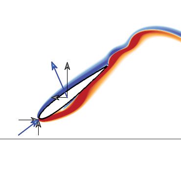
Downloaded from https://www.cambridge.org/core. MIT Libraries, on 09 Jul 2021 at 18:36:23, subject to the Cambridge Core terms of use, available at https://www.cambridge.org/core/terms. https://doi.org/10.1017/jfm.2021.469
D. Fernández-Gutiérrez and W.M. van Rees
ft = 0.750 ft = 0.875 ft = 1.000 ft = 1.125 ft = 1.250
x
θ
y
ac = as = 0 (rigid)
ac = –0.8, as = 0
ac = +0.8, as = 0
ac = 0, as = –0.5
ac = 0, as = +0.5
Figure 2. Horizontal cross-sections taken at z/C = {0.000, 0.175, 0.350, 0.525} under various curvature
regimes obtained within the 2-D parametrization (ac , as ).
The inclusion of the overall chord in (3.5) makes the the imposed LE curvature
distribution independent of the chord length distribution across rays. Further, the
cos(β(v)) factor in the first term accounts for the orientation of each ray, so that ac
controls purely cylindrical deformation modes of the fin. More details on this choice of
parametrization are given in appendix B of the supplementary material.
Combined with our choice of heaving and pitching kinematics, figure 2 demonstrates
the effect of positive and negative values of our two parameters ac and as on the fin shape
variations, with ac = as = 0 corresponding to a rigid fin. Additional 3-D views of the
different shapes mimicking the curvature combinations and time stamps plotted in figure 2
are provided in appendix B.4 in the supplementary material.
3.3. Numerical settings
To construct the fin shape we use numerical parameters dist = 5 × 10⁻⁸ and smth =
8 × 10⁻⁷ , and we demonstrate in appendix C.1 of the supplementary material that the
associated time-varying mid-surface area changes are negligible.
921 A22-10Downloaded from https://www.cambridge.org/core. MIT Libraries, on 09 Jul 2021 at 18:36:23, subject to the Cambridge Core terms of use, available at https://www.cambridge.org/core/terms. https://doi.org/10.1017/jfm.2021.469
Effect of curvature actuation on flapping fin performance
The spatial resolution throughout the simulations is set by a uniform grid spacing
of x = C/200, following the grid convergence analysis presented in appendix C.2
in the supplementary material. The temporal resolution is fixed by a Lagrangian
Courant–Friedrichs–Lewy (LCFL) time step constraint of LCFL = 0.1 (van Rees et al.
2011). The computational domain increases dynamically to capture the support of the
vorticity field as the wake grows.
The time-varying thrust, lift and power coefficients are defined as
T(t)
CT (t) = 2
, (3.6)
0.5ρAU∞
L(t)
CL (t) = 2
, (3.7)
0.5ρAU∞
P(t)
CP (t) = 3
, (3.8)
0.5ρAU∞
where T, L and P are the thrust, lift and power computed from the flow field at a given time
step following equations (2.19), (2.20) and (2.22), and A is the reference fin area taken as
twice the mid-surface area to approximate the wetted surface area.
The imposed rigid-body kinematics are ramped up during the first flapping period
through multiplication with a quarter period of a sine function. We then simulate
until non-dimensional time ft = 1.5, and compute the cycle-averaged thrust and power
coefficients (CT and CP , respectively) over the last simulated half-cycle (1 ft 1.5)
1.5/f
CT = CT (t) dt, (3.9)
t=1/f
1.5/f
CP = CP (t) dt. (3.10)
t=1/f
We can then define the propulsive efficiency as
CT
η= . (3.11)
CP
Appendix C.3 of the supplementary material validates this choice of measurement
window, and demonstrates that, with our chosen ramp up, the force and power coefficients
have already reached their steady-state values after the first cycle.
In the following, we will primarily rely on CT , CP and η, as defined above, as metrics
for hydrodynamic performance.
4. Effect of curvature variations on hydrodynamic performance
Using the numerical framework and heave/pitch kinematics as described above, we
simulated a set of flapping fins with curvature parameter variations ac ∈ [−0.4, 0.8] and
as ∈ [−0.5, 0.75], with ac = as = 0 corresponding to a rigid fin. For each simulation, we
recorded the mean thrust and power coefficients, and computed the propulsive efficiency.
These results are shown as contour plots in figure 3, visualizing the effect of changing the
curvature parameters on the hydrodynamic performance metrics.
921 A22-11Downloaded from https://www.cambridge.org/core. MIT Libraries, on 09 Jul 2021 at 18:36:23, subject to the Cambridge Core terms of use, available at https://www.cambridge.org/core/terms. https://doi.org/10.1017/jfm.2021.469
D. Fernández-Gutiérrez and W.M. van Rees
(a) CT (b) CP
0.1
0.18
0.1
4
0.1
0.10
2
0.08
0
4
7
0.1
1.5
2
1.0
0.1
0.5
0.6 0.6
0.882
2.5
2.0
0.164
0.16
16
0.
0. 1
0.4 0.14 0.4
6
0.18 2.0
0.06
0.144
0.12
0.164
0.2 0.2
0.12
0.164
0.14
00.112
0.10
1.5
0.08
0.827
1.5
2.0
2.5
0.55
1.0
as 0 00.16 0.10
0
8
0.1
0.08
0.16
0.18
1.0
–0.2 –0.2
0
0.1
0.06
4
4
0.1
16
8
2
0.
0.0 0.0
0.1
0.5
0.1
–0.4 0.04 –0.4
0..14
6
6
00.12
00.10
4
1.5
2.5
1.00
2.0
0.5
0.16
–0.4 –0.2 0 0.2 0.4 0.6 0.8 –0.4 –0.2 0 0.2 0.4 0.6 0.8
η
(c)
0.10
0.08
0.12
0.06
0.14
0.199
0.222
0.18
0.6
00.16
0.118
0.20
1
9
0.19
0.4
0.22
0.15
0.2
0.10
0.06
0.08
00.12
0.14
as
9
2
0.18
0.19
0.2
0.116
0 0.10
0.1
99
4
0.0
–0.2
0.18 0.05
0
6
4
2
8
–0.4
0.1
0..0
0.1
0..1
0..0
6
0.1
–0.4 –0.2 0 0.2 0.4 0.6 0.8
ac
Figure 3. Cycle-averaged thrust (a) and power (b) coefficients and efficiency (c) results from Navier–Stokes
simulations (black dots), and an interpolated contour plot based on these results, as a function of the two
curvature parameters ac and as .
Based on figure 3, the maximum computed thrust occurs at ac = 0.3 and as = 0.1, and
is approximately 15 % larger than that for a rigid fin. Further, we can see that positive
values of ac generally improve the thrust coefficient up until the maximum, after which
the thrust coefficient decays. The effect of spanwise curvature variations, as measured by
as , is less pronounced than the chordwise curvature effect.
For efficiency, the maximum occurs at ac = −0.2 and as = 0.25, leading to
approximately 18 % improvement over the rigid fin. The increase in efficiency is driven
by a strong decrease of the power coefficient as ac decreases. We also observe a small
reduction of the power with increasing spanwise curvature parameter, so that the maximum
efficiency is achieved at positive as .
Figure 4 shows the vortical structures at ft = 1.5 for the rigid fin, and the conditions
corresponding to maximum computed thrust and maximum computed efficiency,
respectively. We observe an increase in the intensity of the vortices shed from the fin
for the maximum thrust, whereas the maximum efficiency case has a much smaller wake
signature.
5. Analysis of the effect of curvature variations
In the following two subsections, we investigate in detail the effect of our chordwise and
spanwise curvature parameters on the hydrodynamic performance of the fin, guided by the
above observations.
921 A22-12Downloaded from https://www.cambridge.org/core. MIT Libraries, on 09 Jul 2021 at 18:36:23, subject to the Cambridge Core terms of use, available at https://www.cambridge.org/core/terms. https://doi.org/10.1017/jfm.2021.469
Effect of curvature actuation on flapping fin performance
(a) (b) (c)
Rigid
Max CT
Max η
Figure 4. Fin shape (a), ωz vorticity field at v = 0 (b) and 3-D vorticity field (c) for the rigid configuration
(top, ac = 0.0, as = 0.0), the maximum thrust configuration (middle, ac = 0.3, as = 0.1) and the maximum
efficiency configuration (bottom, ac = −0.2, as = 0.5), all at ft = 1.5. The 3-D flow structures are visualized
using vorticity magnitude, and both 2-D and 3-D visualizations are coloured by ωz . Animations of the flow
fields of these three cases are given in the supplementary material as movies 2–4, respectively.
5.1. Effect of chordwise curvature parameter ac
As shown in the previous section, chordwise deformation has the largest impact on both
thrust and power, which is qualitatively consistent with previous results (Zhu & Shoele
2008; Esposito et al. 2012). In this section we focus on the underlying mechanisms by
considering only configurations with as = 0.
Geometrically, by varying ac , the mid-surface plane rolls over a vertical cylinder of
radius C/ac . As ac increases, this means the curving fin is different from the reference
rigid fin in two aspects. First, the line connecting leading and trailing edge of the fin
also undergoes additional lateral trailing-edge excursions (see figure 5). Second, on top
of the modified trailing-edge kinematics, the fin experiences a camber-like deformation.
The former effect can be described as an additional pitching contribution, on top of
the reference pitching kinematics (3.2). Based on the deformation mode considered, this
additional pitching term can be derived as θκ (t) = 0.5ac sin(2πft). With this insight, we
can then decompose the effect of ac into two characteristics: the first increases the pitch
variations of the reference rigid fin with θκ (t), and the second adds the chordwise curvature
on top of this rigid-body motion without affecting the leading- and trailing-edge locations.
We investigate the first effect by simulating a rigid fin undergoing altered pitch
kinematics given by
θ κ-pitch (t) = −Aθ cos(2πft) + 0.5ac sin(2πft), (5.1)
921 A22-13Downloaded from https://www.cambridge.org/core. MIT Libraries, on 09 Jul 2021 at 18:36:23, subject to the Cambridge Core terms of use, available at https://www.cambridge.org/core/terms. https://doi.org/10.1017/jfm.2021.469
D. Fernández-Gutiérrez and W.M. van Rees
(a) 0.6 (b) (c)
0.4 0.5 0.5
0.2
y θκ 0 0
0
–0.2 –0.5 –0.5
0 0.5 1.0 0 0.5 1.0 0 0.5 1.0
x x x
Figure 5. (a) Horizontal cross-sections at ft = 1.25 of the curved fin with ac = 0.8 and as = 0. (b,c)
Cross-sections at v = 0 of the curved (b) and κ-pitch (c) configurations during the down-stroke half-cycle,
visualized at seven equidistant time instances between ft = 0.25 (lightest) and ft = 0.75 (darkest).
(a) (b) (c)
5 0.25
0.30 4 0.20
0.25 Curved
κ-pitch CP
3 η 0.15
CT 0.20
2 0.10
0.15
0.10 1
0.05
0.05 0
–0.5 0 0.5 1.0 1.5 –0.5 0 0.5 1.0 1.5 –0.5 0 0.5 1.0 1.5
ac ac ac
Figure 6. Cycle-averaged thrust coefficient (a), power coefficient (b) and efficiency (c) as a function of the
chordwise curvature parameter ac , for the fin with curvature variations (in blue) and the rigid fin with κ-pitch
kinematics (in orange).
while keeping the geometry and heave kinematics the same as the reference rigid fin. This
configuration, which we denote as the κ-pitch case, is also parametrized by ac , although
the fin does not undergo any curvature variations.
Figure 6 compares the thrust, power and efficiency of the curved and κ-pitch
configurations for the range of ac studied, where again ac = 0 corresponds to the rigid
fin with unaltered pitching kinematics. We observe that the κ-pitch case qualitatively
reproduces the effect of ac on the mean thrust coefficient, leading to a decrease in thrust
for negative values and the existence of a maximum at finite ac > 0. The effect of ac on
power and efficiency are also qualitatively comparable between the curved and κ-pitch
configurations. This provides our first insight into why the chordwise curvature variations
lead to increased thrust coefficient.
However, quantitatively there is a significant increase in the maximum thrust coefficient
achieved by the κ-pitch case over the optimally curved case. Further, the peak thrust for the
κ-pitch fin occurs at ac = 0.95, vs ac = 0.28 for the curved fin. Since power consumption
is approximately equal between the two cases, the efficiency of the κ-pitch fin at high thrust
values (ac > 0) is significantly higher than for the curved fin. The optimal efficiency, on
the other hand, is achieved at much lower thrust values – here, the curved fin outperforms
the κ-pitch fin slightly, which we will discuss more at the end of this subsection.
To understand why the κ-pitch kinematics are able to practically double the thrust
coefficient (at ac = 0.8) of the reference rigid fin (ac = 0), figure 7(a) compares the
pitch angle variations as a function of time for the reference rigid fin (in red) and the
κ-pitch fin (in orange). Note that, by construction, the pitch angle variations of the κ-pitch
configuration (in orange) are identical to that of the curving fin (in blue) at equal values
921 A22-14Downloaded from https://www.cambridge.org/core. MIT Libraries, on 09 Jul 2021 at 18:36:23, subject to the Cambridge Core terms of use, available at https://www.cambridge.org/core/terms. https://doi.org/10.1017/jfm.2021.469
Effect of curvature actuation on flapping fin performance
(a) (b) 6
40
4
20
2
θ (deg.)
0 v(TE)
y
0
Rigid –2
–20 Curved ac = 0.8
κ-pitch ac = 0.8 –4
Rigid Aθ = 35°
–40 Rigid ϕθ = –45°
–6
1.0 1.2 1.4 1.6 1.8 2.0 1.0 1.2 1.4 1.6 1.8 2.0
ft ft
Figure 7. Pitch angle (a) and trailing-edge lateral velocity (b) during a flapping cycle, for the rigid fin with
reference kinematics (red), the fin with curvature variations ac = 0.8 (blue) and the rigid fin with κ-pitch
kinematics using ac = 0.8 (orange). Also shown are the rigid fin results with harmonic pitch variations with
amplitude Aθ = 35◦ (brown) and with phase shift ϕ = −45◦ (grey).
of ac . The plot shows how, compared with the reference rigid fin, the κ-pitch configuration
not only achieves an increase in maximum pitch angle, but also affects the phase shift with
the heave motion. In fact, we can estimate the effective pitch amplitude and phase values
of the κ-pitch kinematics, using (5.1), as follows:
κ-pitch
Aθ = max(θ) = A2θ + (0.5ac )2 , (5.2)
κ-pitch
π 0.5ac
ϕθ = 2π tmax(θ ) − tmax( y) = − arctan . (5.3)
2 Aθ
For ac = 0.8, where the κ-pitch kinematics achieve maximum thrust, we then find
κ-pitch κ-pitch
Aθ = 37.8◦ and ϕθ = −52.6◦ .
When analysing the isolated effect of pitch amplitude and phase angle variations on
our reference rigid fin, we see why the altered kinematics of the κ-pitch configuration
are virtuous. Appendix D.1 in the supplementary material shows that changing the phase
shift from −90◦ to −45◦ doubles the thrust coefficient of the reference rigid fin, and an
independent increase in pitch amplitude from 30◦ to 35◦ also leads to a modest increase
in thrust. The corresponding pitch angle variations are shown in figure 7(a) as the grey
and brown lines, respectively. The κ-pitch configuration then combines a pitch amplitude
and pitch phase shift that are very close combinations of the individual optimal values for
the reference rigid fin with sinusoidal pitch variations. As a side note, we observe also in
appendix D.1 in the supplementary material that in terms of efficiency, the −90◦ phase
angle is optimum, consistent with the findings of Read et al. (2003).
To summarize results so far, we have observed that the original curvature variation,
as dictated by ac , provides an altered pitching kinematics that increases the mean thrust
coefficient achieved by the fin. We can reproduce this effect with a rigid fin, both using a
combined effective amplitude and phase shift, as well as through independent variations of
amplitude and phase shift. Both indicate that the significant driver in thrust increase is the
phase shift change from −90◦ to approximately −50◦ . In the remainder of this subsection
we will focus on two open questions: the first asks why this altered pitching kinematics
improves performance, and the second asks why the κ-pitch fin provide significantly larger
thrust values for all ac > 0 compared with the curving fin.
921 A22-15Downloaded from https://www.cambridge.org/core. MIT Libraries, on 09 Jul 2021 at 18:36:23, subject to the Cambridge Core terms of use, available at https://www.cambridge.org/core/terms. https://doi.org/10.1017/jfm.2021.469
D. Fernández-Gutiérrez and W.M. van Rees
We answer the first question by examining the trailing-edge (TE) lateral velocity
as shown in figure 7(b) for all cases discussed above. From (3.1), (3.2), and (5.1),
(TE)
we find that the maximum TE velocity, scaled by chord and frequency, is vy,max ≈
2π (Ãy + 0.5ac )2 + A2θ . For our parameter choices, the amplitude of the TE lateral
velocity increases approximately 1.45-fold between the reference rigid fin and the κ-pitch
configuration with ac = 0.8, leading to an increase in mean thrust coefficient by a factor
of 2.1. This is consistent with the added mass effect for pitching fin propulsion (Garrick
1936; Gazzola, Argentina & Mahadevan 2014b; Smits 2019) which predicts that the thrust
coefficient is proportional to the square of the lateral velocity. The TE velocity amplitude
does not solely predict performance: the timing of maximum TE velocity compared with
the fixed heaving kinematics also affects the thrust coefficient. This is a much more subtle
interaction, however, that would require further investigation.
The second open question concerns the difference between the fin with curvature
variations and the κ-pitch configuration, for the same value of ac . To address this,
we plot the time evolution of the difference in thrust and lift coefficients between the
curving fin and the κ-pitch configuration in figure 8(a). For reference, the time evolution
of the individual force coefficients is included in appendix D.2 in the supplementary
material. From figure 8(a), we can identify two reasons for the lower thrust coefficient
of the chordwise curving fin compared with the κ-pitch fin. First, for times 1 ft
1.2, corresponding to the second half of the upstroke just before reversal of the heave
kinematics, the difference in CT is large whereas the difference in CL is relatively small.
This implies an increased drag force on the curving fin, consistent with the curved profile
in this part of the stroke where the fin becomes aligned with the inflow. The images on
the top row of figure 8(b) confirm that the total force vector is angled more vertically
for the curved case compared with the κ-pitch case. Second, for times 1.25 ft 1.5,
corresponding to the first part of the downstroke after the heave motion has reversed,
we observe that the κ-pitch configuration experiences both larger thrust and larger lift
coefficients. This means that the overall force vector on the fin is larger for the κ-pitch
fin. We attribute the decreased force of the chordwise curving fin to the camber, which
essentially is ‘reversed’ as the trailing edge slopes upwards, in the direction of the force
resultant. The images on the bottom row of figure 8(b) corroborate this visually. Both
of these effects are repeated every ft = 0.5 times due to the symmetry of the up- and
down-strokes. These two reasons (additional profile drag and reverse camber) lead to the
reduced performance of the chordwise curving fin compared with the κ-pitch rigid fin.
So far, this subsection has focused on the regime ac > 0, where significant gains in
the mean thrust coefficient are observed. However, our results also show that negative
values of ac monotonically decrease the power required to move the fin, and increase
the efficiency η. The power reduction is apparent from figure 9, showing the power
components associated with heave and pitch, defined as P(L) = −Lẏ and P(M) = −M · θ̇,
respectively. The plot demonstrates that the power reduction is approximately equally
distributed between the heave and pitch kinematics. The deformation-related power
def
coefficient, CP = CP − CPT − CPM , decreases as well, but this reduction is relatively
insignificant compared with the other two components. To distinguish the effects of fin
camber and TE kinematics in the regime ac < 0, we can revisit figure 6. Both the κ-pitch
and the curving fins reduce their power coefficients equally, indicating that the power
reduction at negative ac is due to the reduced TE velocity. However, only the curving
fin demonstrates a peak in efficiency at ac < 0, since the fin camber leads to a slight
increase in thrust coefficient over the κ-pitch configuration for the same values of ac .
Consequently, the efficiency peak of the curving fin is higher than that of any of the rigid
921 A22-16Downloaded from https://www.cambridge.org/core. MIT Libraries, on 09 Jul 2021 at 18:36:23, subject to the Cambridge Core terms of use, available at https://www.cambridge.org/core/terms. https://doi.org/10.1017/jfm.2021.469
Effect of curvature actuation on flapping fin performance
(a) 0.6 (b)
CT(κ–pitch) – CT(curved)
CL(κ–pitch) – CL(curved)
f t = 1.1
0.4
0.2
0
–0.2
f t = 1.4
–0.4
1.0 1.2 1.4 1.6 1.8 2.0 Curved ac = 0.8 κ-pitch ac = 0.8
ft
Figure 8. (a) Difference in thrust and lift coefficients between the curved and κ-pitch configurations with
ac = 0.8. Solid and dashed lines identify the upstroke and downstroke half-cycles, respectively. (b) Vorticity
contours at the centre plane. Incident velocity vector and its horizontal and vertical components annotated at
the LE (u = [U∞ , −ẏ]). Fluid force vector and its horizontal and vertical components annotated at fin centroid
(F = [−T, L]).
(a) CP(L) (b) CP(M)
1.1
0.9
0.4
0.5
0.7
0.8
0.6
1.00
0.3
0.6 1.2 0.6 0.9
6
0.48
3
5
0.
0.3
1 0.
0.
0.2
1.0 0.6 0.8
0.4 0.4
0.7
00.47
11.2
0.2 0.8 0.6
477
0.2
11.11
1.0
0.486
0.8
0.9
0.7
0.6
0.5
0.3
0.4
0.3
0.5
0.5
as 0 0.7
0.3
0.6
8
0.2
0.
0.6 0 0.4
–0.2 0.4 –0.2 0.3
11.33
0.2
0.47
1.2
0.2
0.486
0.7
0.5
0.3
0.9
–0.4 –0.4
0.3
0.6
0.8
0.2 0.1
1.0
1
–0.4 –0.2 0 0.2 0.4 0.6 0.8 –0.4 –0.2 0 0.2 0.4 0.6 0.8
ac ac
Figure 9. Cycle-averaged power coefficient components linked to heave (a) and pitch (b) computed from
Navier–Stokes simulations (black dots), and an interpolated contour plot based on these results, as a function
of the two curvature parameters ac and as .
fins, and achieved at a negative ac value. Overall, this behaviour is consistent with intuition
– negative values of ac correspond to curvature ‘with the flow’, i.e. qualitatively similar to
elastic deformation, as well as a hydrodynamically beneficial camber induced during the
thrust-generation part of the stroke.
5.2. Effect of spanwise curvature parameter as
As discussed previously, spanwise curvature variations as parametrized by as
predominantly affect the cycle-averaged power coefficient, which monotonically decreases
with increasing values of as within the range of curvatures simulated. Figure 9 shows
that this power reduction originates almost exclusively from the pitch kinematics. In this
section we will investigate this effect further, considering only configurations with ac = 0.
921 A22-17Downloaded from https://www.cambridge.org/core. MIT Libraries, on 09 Jul 2021 at 18:36:23, subject to the Cambridge Core terms of use, available at https://www.cambridge.org/core/terms. https://doi.org/10.1017/jfm.2021.469
D. Fernández-Gutiérrez and W.M. van Rees
(a) (b) (c)
0.20 1.2 0.22
Curved
0.18 κ–twist
1.0 0.20
— 0.16 —
CT CP 0.8 η 0.18
0.14
0.12 0.6 0.16
0.10 0.4 0.14
–0.5 0 0.5 1.0 –0.5 0 0.5 1.0 –0.5 0 0.5 1.0
as as as
Figure 10. Cycle-averaged mean thrust coefficient (a), mean power coefficient (b) and efficiency (c) as a
function of the spanwise curvature parameter as , for the fin with curvature variations (blue) and the κ-twist
configuration (green).
Similar to the chordwise curvature in the previous section, the spanwise curvature can
be decomposed into two components: the spanwise twisting of otherwise straight rays, and
the actual curving of the rays without further affecting their TE locations. We can isolate
the former component starting from a rigid fin, and adjust the pitch variation across the
height of the fin to match the LE–TE direction associated with the as curvature profile
!
θ κ-twist (v, t) = −Aθ + 0.5as v 2 cos(2πft). (5.4)
We name this configuration κ-twist, and note that we have to relax the membrane
inextensibility constraint to accomplish the resulting shape.
Figure 10 compares the behaviour of the deformed fin with that of the κ-twisted fin,
across the range of as values considered. The qualitative trends are similar, with increasing
as values increasing thrust, decreasing power and increasing efficiency for both the curving
and the κ-twist fins. This demonstrates that the spanwise twist is the predominant factor
underlying these hydrodynamic characteristics, rather than the actual curvature of the rays.
We observe a slight increase in peak efficiency of the curving fin compared with the
κ-twist configuration indicating that here, again, the camber can improve efficiency.
To understand the effect of κ-twist kinematics on the performance, we can examine (5.4)
further. For our spanwise curvature parametrization, the spanwise curvature variations are
in phase with pitch but of the opposite sign. Positive values of as then decrease the effective
pitch angle, and vice versa, with the maximum effect noticeable at the top and bottom
of the fin, away from the centre plane. This is observed in figure 11, showing that the
pitch angle and TE velocity amplitude of the top ray during a flapping cycle significantly
reduces when as is increased. Consequently, since the outer parts of the fin undergo
smaller pitching amplitudes, the associated power reduction is observed predominantly
in the pitching component CPM . Further, the reduced power and increased efficiency with
increasing spanwise curvature parameter are consistent with the smaller vortical signature
of the wake, as shown in figure 12. The twisted configuration with as = 0.5 leads to
significantly smaller tip vortices shed from the outer edges of the fin, compared with both
rigid and as = −0.5. Lastly, we note that the qualitative deformation of the fin when as > 0
is intuitively consistent with the elastic deformation of a finite-span flapping fin: the outer
edges will curl inwards during the heave reversal, lagging behind the central rays of the
fin. Together with the previous results, this provides further indication that the curvature
variations of passively deforming 3-D fins can lead to higher propulsive efficiency than
those of rigid fins, as measured solely through hydrodynamic performance.
921 A22-18You can also read