Improving MACD Technical Analysis by Optimizing Parameters and Modifying Trading Rules: Evidence from the Japanese Nikkei 225 Futures Market - MDPI
←
→
Page content transcription
If your browser does not render page correctly, please read the page content below

Journal of
               Risk and Financial
               Management

Article
Improving MACD Technical Analysis by Optimizing
Parameters and Modifying Trading Rules: Evidence
from the Japanese Nikkei 225 Futures Market
Byung-Kook Kang

                                           Department of Business Administration, Nanzan University, Aichi 466-8673, Japan; kangbk@nanzan-u.ac.jp

                                           Abstract: Much research has examined performance or market efficiency by using the moving
                                           average convergence divergence (MACD) technical analysis tool. However, most tests fail to verify
                                           efficiency with the traditional parameter settings of 12, 26, and 9 days. This study confirms that
                                           applying the traditional model to Japan’s Nikkei 225 futures prices produces negative performance
                                           over the period of 2011–2019. Yet, it also finds that the MACD tool can earn significant positive
                                           returns when it uses optimized parameter values. This suggests that the Japanese market is not
                                           weak-form efficient in the sense that futures prices do not reflect all public information. Hence, the
                                           three parameters values of the MACD tool should be optimized for each market and this should
                                           take precedence over finding other strategies to reduce false trade signals. This study also tests
                                           which models are able to improve profitability by applying additional criteria to avoid false trade
                                           signals. From simulations using 19,456 different MACD models, we find that the number of models
                                           with improved performance resulting from these strategies is far greater for models with optimized
                                           parameter values than for models with non-optimized values. This approach has not been discussed
                                           in the existing literature.


                                           Keywords: MACD; technical analysis; trading simulation; buy-and-hold strategy; market efficiency;
Citation: Kang, Byung-Kook. 2021.          Nikkei 225 futures
Improving MACD Technical Analysis
by Optimizing Parameters and
Modifying Trading Rules: Evidence
from the Japanese Nikkei 225 Futures       1. Introduction
Market. Journal of Risk and Financial
                                                 MACD (Moving Average Convergence Divergence) is one of the most popular mo-
Management 14: 37. https://doi.org/
10.3390/jrfm14010037
                                           mentum indicators used in the technical analysis of the prices of stocks and other tradeable
                                           assets. It consists of three parameters to define three time-periods: two parameters are
Received: 21 December 2020
                                           for the calculation of the MACD series which is the difference between the ‘short-term’
Accepted: 12 January 2021                  and ‘long-term’ exponential moving averages (EMA) of the price series; the other is for
Published: 16 January 2021                 the ‘Signal’ of the series which is an EMA of the MACD. All the series are calculated from
                                           historical price data, most often using daily closing prices, and illustrated as a “MACD
Publisher’s Note: MDPI stays neu-          line” and a “Signal line” on a graphic chart of the indicator. In terms of signal generation,
tral with regard to jurisdictional clai-   it is common to interpret it as follows: ‘buy’ when the MACD line crosses up through
ms in published maps and institutio-       the Signal line and ‘sell’ when it crosses down though the Signal line. This trading rule
nal affiliations.                          is called a “signal line crossover” and the buy/sell signal is considered to be a primary
                                           cue provided by the indicator, although the actual ways investors use the MACD model to
                                           trade are diverse.
                                                 The most commonly used parameter values are 12, 26, and 9 days, and these values are
Copyright: © 2021 by the author. Li-
                                           usually represented in the form MACD (12,26,9). However, the (12,26,9) format is neither
censee MDPI, Basel, Switzerland.
                                           a formal standard nor a combination recommended by Appel (1979) who developed the
This article is an open access article
distributed under the terms and con-
                                           MACD. It is said that Appel originally suggested two different settings on a daily chart:
ditions of the Creative Commons At-
                                           (8,17,9) for buy signals and (12,25,9) for sell signals. Murphy (1999, p. 253) later mentioned
tribution (CC BY) license (https://        these two different setting values of Appel and added: “Appel originally recommended
creativecommons.org/licenses/by/           one set of numbers for buy signals and another for sell signals. Most traders, however,
4.0/).                                     utilize the default values of 12, 26, and 9 in all instances”. In fact, each element of (12,26,9)

J. Risk Financial Manag. 2021, 14, 37. https://doi.org/10.3390/jrfm14010037                                    https://www.mdpi.com/journal/jrfm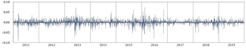
J. Risk Financial Manag. 2021, 14, 37                                                                                            2 of 21

                                        represented—in those times when the work week consisted of 6 days, not 5 days—2 trading
                                        weeks, 1 trading month, and one and a half trading weeks, respectively. However, all
                                        signals generated by the MACD indicator depend on the three parameter values. Therefore,
                                        other values can be substituted according to one’s trading style and goals in a way to
                                        change the sensitivity of the signal generation process.
                                              Nonetheless, many academic researchers have tested the effectiveness of the MACD
                                        approach or used it to measure market efficiency. However, quite a few of these evaluations
                                        failed to verify efficiency based on trading results obtained with its three traditional param-
                                        eter settings of 12, 26, and 9 days. They focused their attention on testing whether applying
                                        technical analysis tools such as the MACD indicator to financial markets can produce better
                                        returns than non-technical buy-and-hold strategies or the risk-free interest rate. Hence,
                                        little attention has been given to explaining the optimality of the MACD’s traditional
                                        parameter value settings. Some researchers utilized different parameter combinations, but
                                        they also did not provide any rationale for their values, except for vague words such as,
                                        ‘because it is most commonly used’. This suggests that if they had considered other values,
                                        they may have reached very different conclusions. So there is room to improve the existing
                                        approach for tests of market efficiency using the MACD.
                                              On the other hand, the attention of practitioners who utilize the MACD indicator is
                                        focused on improving its profitability. Hence, they seek optimal parameter values to obtain
                                        the best result. However, it is not easy to test different parameter values because there are
                                        too many different potential combinations. Broadly speaking, the main reason to persist
                                        in using common parameter values is the momentum of tradition. Meanwhile, when the
                                        predictive power of the MACD (12,26,9) model degrades, they question its trade signals
                                        and try additional trading strategy criteria to modify these degraded trade signals. In
                                        fact, one approach to reduce false trade signals is changing the parameter settings of the
                                        MACD to control directly the frequency of signal generation. Another approach is using
                                        additional trading strategy criteria to modify indirectly the trade signals produced by the
                                        trading rule. However, additional strategies are often based on individual experience and
                                        intuition with no consistency. Here arises some simple questions, “Do these supplemental
                                        trading strategies make it possible to improve profitability by reducing false trade signals,
                                        without changing the traditional parameter values? Or, should the traditional parameters
                                        of the MACD model be changed to reduce false trade signals?
                                              From this point of view, the goal of this research is to examine the validity of the
                                        following three points:
                                        (1)   Whether the application of the traditional MACD model to investing in the Japanese
                                              stock market produces genuine profits.
                                        (2)   Whether substituting more-optimized, better-fitted parameter values for the tradi-
                                              tional ones can deliver higher returns than the traditional model.
                                        (3)   Whether applying additional strategies to avoid false trade signals to the models with
                                              optimized parameter values improves profitability. And, to be more specific:
                                              •   Whether a systematic trading strategy adapted to the models with better-optimized
                                                  parameter values is able to produce significantly higher returns compared to the
                                                  traditional model and a non-technical buy-and-hold strategy.
                                              •   Whether the effect of applying a systematic trading strategy can be an improve-
                                                  ment, even for models with non-optimized parameter values.
                                              There are many published papers using the MACD model. However, little attention
                                        has been given to the third point mentioned above (especially to the last sub-point). In
                                        this respect, this research is a comparative analysis of the effects of applying additional
                                        strategies to the optimized parameter settings and non-optimized settings. Several useful
                                        findings and suggestions arise from this research.
                                              The remainder of the research is structured as follows: Section 2 reviews the existing
                                        literature related to this research. Section 3 briefly explains the MACD momentum indicator
                                        and the limitations caused by false signal generation. Section 4 details the methodology
                                        employed in this study. Section 5 presents empirical results on the aforementioned three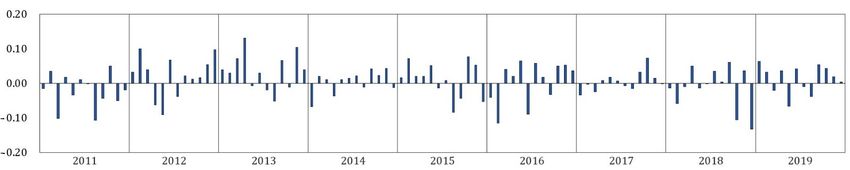
J. Risk Financial Manag. 2021, 14, 37                                                                                             3 of 21

                                        points and comments on them. Section 6 provides concluding remarks with discussion of
                                        the implications of the research.

                                        2. Literature Review
                                              Many academic researchers adopted the traditional parameter values to test the
                                        effectiveness of the MACD approach and measure market efficiency based on the efficient
                                        market hypothesis (EMH) of Fama (1970). Chong and Ng (2008) examined the MACD
                                        model and another technical analysis tool, the Relative Strength Index (RSI) to see if these
                                        trading rules are profitable. Using 60 years of data (1935–1994) for the London Stock
                                        Exchange FT30 index, they found that the two trading tools can generate higher returns
                                        than a buy-and-hold strategy in the market. The “buy-and-hold” strategy was applied as a
                                        benchmark to test the effectiveness of both the MACD and the RSI, which focus on 10-day
                                        returns following a buy or sell signal while then ignoring all other transaction signals over
                                        these 10 days. In terms of the MACD, they adopted an MACD (12,26,0) model which
                                        follows a “zero crossover” trading rule (see Section 3.2 for the details). The reason for
                                        adopting this form of the MACD (12,26,0) model was simply because “12- and 26-day are
                                        the most commonly used”, as quoted by Murphy (1999).
                                              Chong et al. (2014) later examined whether the MACD model and RSI can generally
                                        generate excess returns for the stock markets of five other OECD countries (Italy, Canada,
                                        Germany, United States and Japan). They applied MACD (12,26,0), MACD (12,26,9) and
                                        MACD (8,17,9) models to market data over 27 years (1976–2002). Their findings were:
                                        (1) the MACD (12,26,0) model outperforms a buy-and-hold strategy in the Italian (Milan
                                        Comit General) and Canadian (S&P/TSX Composite Index) stock markets; (2) using the
                                        traditional MACD (12,26,9) model led to significant negative returns for the German (DAX
                                        30) stock market and the model had no predictive power for the other countries’ markets;
                                        and, (3) the returns of the MACD (8,17,9) model—which was introduced by Appel—were
                                        significantly negative in the Italian and German markets while it had no predictive power
                                        for the other markets. Based on these findings, they concluded that the MACD (12,26,0),
                                        MACD (12,26,9), and MACD (8,17,9) trading rules are “not robust to the choice of market”.
                                        But what we should not overlook here is that while the MACD (12,26,0) trading rule
                                        outperformed the buy-and-hold strategy in the Italian market, the MACD (12,26,9) model
                                        did not show profit potential in the same market. This is strong evidence that suggests
                                        that the profitability of the MACD approach will depend on its parameter value settings.
                                        To add a remark in passing for the reason why they tried the MACD (8,17,9) model, it
                                        was just because of the following claim that, “it can produce more reliable buy signals” in
                                        Pring (2002).
                                              Nor and Wickremasinghe (2014) investigated the profitability of the MACD (12,26,9)
                                        model by using a relatively recent data (1996 to mid-2014) for the Australian All Ordinaries
                                        Index (XOA). They compared the returns of the MACD (12,26,9) trading rule with 10-day
                                        returns for a buy-and-hold strategy using the same approach as Chong and Ng (2008) and
                                        Chong et al. (2014). They found that the traditional MACD model generally performs
                                        poorly in the market but that the RSI model showed some profit potential. So, they
                                        concluded that overall “the Australian stock market is not weak-form efficient”. This
                                        brings up the question, “Why is the traditional (12,26,9) model the sole determinant of the
                                        profitability of all MACD models and market efficiency”? There is no compelling reason to
                                        always use the (12,26,9) parameter settings.
                                              Hejase et al. (2017) have also applied the traditional MACD (12,26,9) model to the
                                        stock prices of six Lebanese banks and a real estate company to determine if the MACD
                                        tool is able to deliver higher profits to Lebanese stock traders. What is interesting is that, in
                                        order to avoid false signals after filtering the empirical results over 10 years of data (2004–
                                        2014), they tested three trading strategies different from the typical ‘signal line crossover’
                                        trading rule of the MACD model. The first one is to execute a ‘buy (sell)’ transaction only
                                        when three ‘buy (sell)’ signals are generated on three consecutive days. The second is to
                                        execute a ‘buy (sell)’ transaction only when the MACD line value exceeds (goes below) the
J. Risk Financial Manag. 2021, 14, 37 4 of 21
Signal line value by more than 0.03 which corresponds to a 3 percent margin of safety. The
third strategy is to execute a ‘buy (sell)’ transaction only when the minimum difference
between the MACD line value and the Signal line value exceeds 0.5, 1.1 or 3.5 percent of
the closing price after waiting for three consecutive similar signals. According to their
logic, “the third strategy was proposed due to the fact that the application of the two
aforementioned strategies did not contribute significantly to the reduction of false signals”.
Nevertheless, they found that all three non-conventional strategies did not outperform a
“buy-and-hold” strategy which consisted of simply buying stocks at the beginning of the
period then selling them at the end of the period. Hence, they concluded that, “In the long
run, the MACD dynamic trades do not make sense since their potential profits are less than
the static ‘buy-and-hold’ approach”. Here again arises the question, “Why persist in using
the traditional (12,26,9) parameter settings?” If they had considered other values, they may
have reached different conclusions.
In fact, prior to the above-mentioned studies, many researchers have already reported
that the MACD does not produce good results by setting its parameters to the tradi-
tional values; they were not able to achieve good results by using the traditional MACD
(12,26,9) model.
Meissner et al. (2001) tested the effectiveness of the traditional MACD (12,26,9) model
and found that it results in a surprisingly poor success rate of 32.14 percent for the DOW
30 stocks and 32.73 percent for the individually tested NASDAQ-100 stocks over the 1989–
1999 period. From these results, they concluded that the traditional MACD indicator can
almost be regarded as a contra-indicator. Armour et al. (2010, cited by Anghel 2015) also
tested the traditional MACD (12,26,9) trading rule, including a simple moving average rule
on 20 years of data for the Irish Stock Market Main Index and found that the MACD rule
underperformed the buy-and-hold strategy. Chen and Metghalchi (2012) investigated the
predictive power of 32 models of single, double or triple-indicator combinations based
on the most popular six technical indicators for the Brazilian stock index (BOVESPA)
over the period of 1996 to 2011 and found that none of the trading models, including the
MACD (12,26,9) model, can beat a buy-and-hold strategy. The results did not support
the predictive power of technical analysis, thus they concluded that the Brazilian stock
index was weak-form efficient. Abbey and Doukas (2012) tested whether the MACD (12,24)
model and three other well-known technical analysis indicators were profitable for five
currencies for individual currency traders. Using a proprietary database of 428 individual
currency traders over the period March 2004 to September 2009, they found that the four
popular technical indicators had negative performance and concluded that this result
arose because individual currency traders used well-known technical indicators to trade
currencies, which implied that such currency traders suffer from reduced performance.
Rosillo et al. (2013) examined which of four popular technical analysis tools, including the
traditional MACD (12,26,9) model achieved greater profitability for the companies of the
Spanish Continuous Market from 1986 to 2009. Although they presented just one example
of results for the Telefonica Company, the total net benefits generated by applying the
MACD model were an unsatisfactory 2.48 percent. Du Plessis (2013) examined the MACD
(12,26,9) model and a buy-and-hold strategy to determine which was more effective for the
South African stock market index (FTSE/JSE Top 40) over the period of 2001 to 2010. He
found that the traditional MACD model was less effective than a buy-and-hold strategy.
Based on this result, he stated that the MACD was not an effective investment strategy
using the default settings in the market.
As can be seen from the above discussion, many researchers have failed to find
satisfactory results for the MACD indicator by using its traditional parameter settings
and have drawn negative conclusions for it. Yet, these researchers did not explore the
optimality of the MACD’s traditional parameters.
Based on the above-mentioned points, it is clear that: (1) there is no compelling need
to stick to the traditional parameter value settings, since these parameter values are not a
genuine standard, and further, that there could be more profitable value combinations; (2)J. Risk Financial Manag. 2021, 14, 37 5 of 21
the three parameter values should be selected in a more systematic way, and be specifically
designed for each market, since the trading signals of the MACD model depend on the
parameter values and their profitability is a consequence of these values; and, (3) optimizing
the three parameter values should take precedence over searching for supplementary
trading strategies to avoid false trade signals. Such an approach is both prudent and
far more efficient than blindly searching for strategies at random without the benefit of
parameter optimization.
3. Preliminaries
The formulas for the elements of the MACD indicator and brief remarks about the
limitations of the indicator are presented in this section.
3.1. The MACD Trading Indicator
The MACD trading indicator consists of the following three elements:
• The MACD line: the difference between the short- and long-term exponential moving
averages (EMA).
• The Signal line: an exponential moving average of the MACD line.
• Histogram: a graphical representation of the distance between the MACD line and
the Signal line.
The EMA is defined as:
2
EMAt = ( Pt − EMAt−1 ) + EMAt−1 (1)
n+1
where n is the number of periods for the EMA and Pt indicates the closing day price (index
value) at time t. Let n1 be the number of short-term and n2 be the number of long-term
periods. Then, EMAs of the two different periods can be presented as:
EMAt (n1 ) = (2/(n1 + 1) × ( Pt − EMAt−1 (n1 )) + EMAt−1 (n1 ) (2)
EMAt (n2 ) = (2/(n2 + 1) × ( Pt − EMAt−1 (n2 )) + EMAt−1 (n2 ) (3)
Using the above equations, the three elements of the MACD indicator are formulated
as follows:
MACDt (n1 , n2 ) = EMAt (n1 ) − EMAt (n2 ) (4)
Signalt (n3 ) = (2/(n3 + 1) × ( MACDt (n1 , n2 ) − Signalt−1 (n3 )) + Signalt−1 (n3 ) (5)
Histogramt = MACDt − Signalt (6)
where n3 denotes the period for the EMA calculation of the MACDt series. The MACD
line, the Signal line and the Histogram can be created from Equations (4)–(6), respectively.
As can be seen from the equations, the three elements (the MACD line, the Signal line, and
the Histogram) move above and below the zero line. Again, the MACD indicator depends
on the time constants for the EMAs, which are usually represented in the form of “MACD
(n1 , n2 , n3 )”, e.g., MACD (12,26,9).
3.2. MACD Trading Rules
The two trading rules mentioned in the first section, “zero crossover” and “signal line
crossover” can be expressed as follows:
Buy, when MACDt (t1 , t2 ) = EMAt (t1 ) − EMAt (t2 ) > 0
zero crossover = (7)
Sell, when MACDt (t1 , t2 ) = EMAt (t1 ) − EMAt (t2 ) < 0
Buy, when Histogramt = MACDt − Signalt > 0
signal line crossover = (8)
Sell, when Histogramt = MACDt − Signalt < 0J. Risk Financial Manag. 2021, 14, 37 6 of 21
Some researchers and practitioners use the former. However, the latter will be adopted
in this study since it is more commonly used these days. We will refer to the latter as the
basic MACD trading rule hereafter.
3.3. Limitations of the MACD Model
As is the case with other technical analysis tools, the MACD indicator can generate
false signals. This is because the MACD model is based on moving averages of past prices
that have already taken place. In other words, the MACD model lags the market price to
a greater or lesser degree and thus trend reversals are detected only after they actually
happen. Due to the inherit limitations of this approach to timing, executing a trade at the
point of signal line crossover can turn out to be a false transaction signal. Such situations
often occur when a signal line crossover indicates a potential buying point, but market
conditions are still considered to be bearish. In contrast a false sell signal occurs when the
crossover calls for a sell, but market conditions are still likely to be bullish.
Analysts therefore use a variety of approaches to filter out such false trade signals and
verify valid trade signals. Three different trading strategies were described by Hejase et al.
(2017). However, no matter which approach is taken, one thing is obvious: the more we
try to reduce the frequency of false trade signals, the more likely we are to lose profitable
opportunities—assuming that the MACD model is basically valid. This implies that we
must accept a certain level of false signal generation; nevertheless, we have to improve the
ability to validate transaction signals since there is no perfect way to predict and eliminate
all false signals. One approach is to change the three parameter values of the MACD to
control the frequency of signal generation (i.e., sensitivity). For example, when calibrating
for greater sensitivity, we could use a smaller moving average. Conversely, when adjusting
to have less sensitivity to reduce false trade signals, we might lengthen the moving average.
We can see from this logic that it is important to adjust the three parameter values for
each market.
4. Research Methodology
As described in the Section 1, three types of models are tested in this study: the
model with the traditional parameter value settings, models with different parameter
combinations, and models for which the trading rule is modified by applying a systematic
approach to avoid false signals. The first-, the second- and the third-types of model will
be referred to hereafter as the “traditional model”, “comparative models”, and “modified
models”, respectively. In addition, models with more-optimized, better-fitted parameter
values for the Japanese market will be referred to as the “optimized model”.
This study uses basic trading simulations to determine the profitability of the tested
models. For the test of profitability of all models mentioned above, the daily closing index
values of Nikkei 225 Futures contracts near maturity over the past nine years (4 January
2011 to 30 December 2019) were obtained from an official data provider, JPX Data Cloud
(http://db-ec.jpx.co.jp). The Nikkei 225 includes the top 225 blue-chip companies listed on
the Osaka Exchange of the Japan Exchange Group (JPX); it is the primary yen-denominated
stock index future.
4.1. Common Matters for Trading Simulations
This study adopts the “signal line crossover” trading rule described by Equation (8)
for the test of profitability of all models. As for determining the buying and selling times
in simulation, we execute as follows. When a ‘buy (or sell)’ signal is generated according
to the signal line crossover, a buy (or sell) order for ‘one trading unit’ is executed at the
closing price (index value) on the next day. After having opened a ‘buy (or sell)’ position,
all subsequent identical buy (or sell) signals are ignored. However, when the first opposite
trading signal from the opening position, i.e., ‘sell (or buy)’ signal is generated, the buy
(or sell) position is assumed to be closed out at the closing price reported on the next day.
At the same time, in order to implement the newly generated signal, a new ‘sell (or buy)’J. Risk Financial Manag. 2021, 14, 37 7 of 21
order for one trading unit is assumed to be executed at the same closing price of the same
day. That is, when a position is closed, a reverse trade is automatically executed. Another
assumption made with regard to the calculation of profitability is that all trades must be
settled by the last trading day of the contract.
As previously stated, only one position for ‘one unit’ can be open at a time and all
transactions have to be executed one-by-one sequentially. This means that holding multiple
positions is not permitted after a position is taken. This assumption is for convenience in
calculating trading returns and to facilitate comparisons with the returns of various models
which have different parameter values.
One contract unit on the Nikkei 225 Futures for a large contract is 1000 times the value
of the Nikkei 225 index value and its tick size is 10 Japanese yen (JPY). Therefore, one tick
up for a one-unit contract leads to a positive return of JPY 10,000 (=10 × 1000). On the other
hand, the current round-trip commission for one large contract unit is approximately JPY
330 in the case of an over-the-counter transaction on almost all Japanese trading websites.
Thus, if the index moves 10 ticks (100), the commission of JPY 330 corresponds to, at best
0.33 percent of the positive or negative return of JPY 100,000; in the case of a 100 tick move,
0.033 percent and so on. That is, the round-trip commission of JPY 330 is so small that it
can be ignored, compared to the high leverage at 1000 times the index value. Thus, this
tiny commission will not be taken into consideration in this study. Accordingly, the return
of each transaction is calculated as:
rsell −buy = Psell − Pbuy (9)
where Pbuy and Psell are the closing index values on the days to execute buying and selling
transactions. A positive (negative) value of Equation (9) indicates a profit (loss), which is
applicable in both the case of a long and a short trade. In the following Section 5.6, log
returns are calculated for every transaction to report test results of whether the difference in
the returns between a modified model and the traditional model is statistically significant.
4.2. Tests of the Performance of the Traditional Model
In order to explore the first check point mentioned at the end of Section 1, we divide
the whole sample into three fairly long sub-periods: 2011–2013, 2014–2016 and 2017–
2019 following the approach of Chong and Ng (2008). This means that the calculation of
profitability for every model is carried out in each sub-period separately for robustness in
choice of sample period. That is, we fit the model to a prior set of data and then tested it on
a later out-of-sample set of data.
4.3. Tests of the Performance of the Comparative Models
In order to explore the second check point mentioned at the end of Section 1 and
verify the validity of the first two assumptions stated at the end of Section 2, we search for
new parameter combinations that outperform the traditional MACD (12,26,9) model. For
the purpose, the three parameters of the MACD (n1 , n2 , n3 ) are taken into consideration
over a given range as follows: n1 = {3,4,· · · ,20}, n2 = {5,6,· · · ,40}, n3 = {3,4,· · · ,40}, where
each is at an interval of one day. This approach produces 24,624 (=18 × 36 × 38) unique
sample models in total, starting from the MACD (3,5,3) model and ending with the MACD
(20,40,40) model. However, this approach produces 5168 (=(16 + 15 + · · · + 1) × 38)
irrational models where the value of the short-term parameter is greater than or equal
to the value of long-term parameter. Accordingly, 19,456 (=24,624 − 5168) models are
examined in this study.
Among the models examined in this study, there were many for which the return in
the first subperiod was higher than that of the traditional MACD (12,26,9) model. However,
we evaluated their performance not only on their return but also in terms of the rate of
profitable trades, the rate of unprofitable trades and the number of total trades from the
perspectives of actual traders. By filtering the results of each model, we excluded models
for which returns were high but that had a high ratio of unprofitable trades and/or theJ. Risk Financial Manag. 2021, 14, 37 8 of 21
actual number of total trades was low from the pool of good performance models.1 As
a result, we chose the MACD (4,22,3) model as a good model. It is balanced in terms of
profit acquisition and loss avoidance, and has enough transactions to satisfy traders who
trade on a short-term basis. This is why we chose the MACD (4,22,3) model as an example
model to be compared with the traditional MACD (12,26,9) model.
4.4. Tests of the Performance of the Modified Models
In order to explore the third check point mentioned at the end of Section 1 and
verify the validity of the third assumption stated at the end of Section 2, we prepared
the following three systematic strategies to avoid false signals and compared the effect of
applying the additional trading strategies to the aforementioned MACD (4,22,3) model and
the traditional MACD (12,26,9) model. We will also extend our analysis to other models
with better-optimized parameter values to check the general result. This includes models
with non-optimized parameter values for robustness.
In evaluating the effectiveness of the three modified strategies, a standard t-test is
utilized in this study in line with the existing literature. The null hypothesis of equality
between the mean return of the model with any of the three modified strategies (µ1 ) and that
of the traditional model (µ2 ), i.e., H0 : µ1 = µ2 is tested against the alternative hypothesis
H1 : µ1 > µ2 . The same approach is used for tests of the difference in mean returns for
long (buy signals) and short trades (sell signals) of the two models to be compared.
4.4.1. A: The n-Day Holding Strategy
For the reason stated above, this strategy considers any closing signal(s) generated
according to a signal line crossover within the first few days after opening a position to
be false trade signal(s) and holds the current position for a minimum number of day(s).
Accordingly, the trading rule adopted by this strategy is stated as: to open a position by
following a signal generated by the trading rule of a signal line crossover and to ignore closing
signals generated ‘within a given few days’ and finally then close the position when the next new
closing signal is generated. More formally,
(
Sell : Ht j < 0, j > i + n
Buy : Hti > 0
opening signal = , closing signal = (10)
Sell : Hti < 0 Buy : Ht j > 0, j > i + n
where Ht indicates the histogram at day t; ti is the day that an opening signal is generated;
n is the minimum number of day(s) that the position should be held; and, t j is the day that
a closing signal is generated after the minimum holding period. For parameter setting, we
let n = {1, 2, · · · , 5} in this study. But we will discuss the case of ‘n = 1’ as an example of
the most profitable strategy and we will refer to this strategy as the ‘1-day’ holding strategy
in the following sections.
4.4.2. B: The x%-Line Crossover of y-Day-Histogram Strategy
As another way to avoid the false signals of the MACD, this strategy focuses on
confirming whether the value of the current histogram reaches a certain size relative to
the zero line—not just crossing over the zero line. More specifically, it is stated as: only if
the current histogram crosses up (down) through a x% line extending below (above) the zero line
to the highest (lowest) histogram over the previous y days, go long (short). This strategy can be
expressed as follows, to open a position by following the buy or sell signal stated below
and close the position by following its opposite trading signal:
Buy : Ht > x ∗ min Ht−y , · · · , Ht−1 , Ht , Ht−y , · · · , Ht−1 , Ht 0
1 For example, MACD (5,17,14) produced a higher return than the MACD (4,22,3) model, but its rate of unprofitable trades was higher and the
number of total trades was also lower.J. Risk Financial Manag. 2021, 14, 37 9 of 21
We parameterize x = {0.5, 0.1, · · · , 0.95, 1.00} and y = {5, 6, · · · , 120} to get a total of
2280 strategies. However, we will only discuss the case of x = 0.3(30%) and y = 10 (days),
which is as an example of the most profitable strategy. We will refer to this strategy as
either the ‘30%-line of 10-day’ or the “30%10d” strategy hereafter.
4.4.3. C: The First Peak/Bottom Point of the Histogram Search Strategy
A trader can consider a peak (bottom) point of the histogram as a turning point in the
market trend (trend reversal)—instead of waiting for the histogram to reach a certain size
as a second strategy. When such a situation is considered, this strategy directs the trader to
wait until he/she finds the first apparent peak (bottom) point of the histogram. To be more
specific, it states: only if histogram values over the most recent three consecutive days are all below
(above) the zero line and the histogram of the middle day is the lowest (highest) among the three
days’ histograms, go long (short). This strategy can be formally expressed:
Buy : Ht−1 = min{ Ht−2 , Ht−1 , Ht }, { Ht−2 , Ht−1 , Ht } < 0
(12)
Sell : Ht−1 = max{ Ht−2 , Ht−1 , Ht }, { Ht−2 , Ht−1 , Ht } > 0
We examine other ways to find the first apparent peak (bottom) point over the most
recent five or seven consecutive days’ histograms and furthermore what happens if we
define the turning point of the market as not the first but rather as the second or third
peak (bottom) point. However, as an example of the most profitable strategy, we will
discuss only the case stated above. This strategy is referred to as the search for ‘the
first-peak/bottom-point’ or the ‘1st-pkbm’ strategy hereafter.
5. Empirical Results
In the 19,456 models examined in this study, there were many for which the profitabil-
ity over the full 9 years was higher than that of the traditional MACD (12,26,9) model. Yet,
to enumerate all the better performing models is not the main point and would divert
us from the purpose of this study. Furthermore, there is space here for only one or two
examples. Therefore, as an example of these superior models, returns from the MACD
(4,22,3) model are presented below. From these, we can see that there are more profitable
parameter value settings than the traditional settings. Having made this point, we turn to
see the effect of using the three additional trading strategies (1-day, 30%10d and 1st-pkbm)
to all models examined in this study.
5.1. An Overview of the Nikkei 225 Futures over the Past Nine Years
Before examining the empirical results, let us begin with a simple observation on the
changes in the trends in the Nikkei 225 Futures values. This will help interpret the results
presented below. The thick line at the top of Figure 1 shows how the index changes from
4 January 2011 to 30 December 2019 (which covers 2204 trading days). The bottom three
J. Risk Financial Manag. 2021, 14, x FOR PEER REVIEW 10 of 22
lines show an MACD line (red), a signal line (blue) and a histogram chart (green) for the
traditional MACD (12,26,9) model.
Figureof
Figure 1. Index Value Index Value
1.Nikkei of Nikkei
225 Futures and225 Futures
moving and MACD
average (12,26,9)
convergence over the(12,26,9)
(MACD) past 9 years.
over the past 9 years.
As we can see from the figure, the index value goes up suddenly from the beginning
of 2013 and then manifests a long-term increasing trend to the end of 2019. The latter pe-
riod is quite different from the relatively stable levels of the period before 2013 (in fact,J. Risk Financial Manag. 2021, 14, 37 10 of 21
As we can see from the figure, the index value goes up suddenly from the beginning of
2013 and then manifests a long-term increasing trend to the end of 2019. The latter period
is quite different from the relatively stable levels of the period before 2013 (in fact, the
stable flat trend to the end of 2012 goes back to 2009). This suggests that we should take the
difference in periods into consideration in analyzing and interpreting the trading results.
We therefore divide the whole period, as was stated in Section 4.2, into three sub-periods:
2011–2013, 2014–2016 and 2017–2019.
As for the increasing trend from the beginning of 2013, the following two expansionary
monetary policies seem to have played a role: the first is the third round of quantitative
easing (QE3: September 2012–October 2014) implemented by the Federal Reserve Board of
the United States, and the other is the large-scale asset purchase program started in April
2013 (at a higher level than in previous years) by the Bank of Japan. As for the increasing
trend from the middle of 2016, it seems to be related to the Bank of Japan’s monetary easing
in September 2016, in addition to its negative interest rate policy from January 2016.
5.2. The Performance of the Traditional MACD (12,26,9) Model
Note that the profitability of this model is shown here by its raw returns to facilitate
comparison with the returns of other models to be discussed later.
The first two columns ‘N(Buy)’ and ‘N(Sell)’ in Table 1 indicate the number of long
and short trades; these are the buy and sell signals generated by the trading rule. The next
two columns ‘N(Buy > 0)’ and ‘N(Sell > 0)’ show the number of profitable long and short
trades, where the numbers inside the parentheses show the proportions of the trades that
are profitable. ‘Buy’ and ‘Sell’ show returns from long and short trades, while ‘Buy + Sell’
indicates the total return of those trades. ‘N(Buy) + N(Sell)’ shows the total number of
long and short trades. The last column ‘N(Buy < 0) + N(Sell < 0)’ is the total number of
unprofitable long and short trades, where the numbers inside the parentheses indicate the
proportions of trades that are losses.
Table 1. The Performance of the Traditional MACD (12,26,9) Model.
N(Buy) N(Sell) N(Buy > 0) N(Sell > 0) Buy Sell Buy + Sell N(Buy) + N(Sell) N(Buy < 0) + N(Sell < 0)
Whole period 84 85 33 (0.393) 20 (0.235) 5430 −9610 −4180 169 116 (0.686)
2011–2013 28 29 13 (0.464) 8 (0.276) 3230 −2370 860 57 36 (0.632)
2014–2016 31 31 11 (0.355) 8 (0.276) 780 −4290 −3510 62 47 (0.758)
2017–2019 25 25 9 (0.360) 8 (0.320) 1420 −2950 −1530 50 33 (0.660)
The first point to observe is that the MACD (12,26,9) model earns a surprisingly
large ‘minus 4180’ for the whole period, which means a capital loss of JPY 4,180,000
(=4180 × 1000, approximately 40,200 US dollars based on the current exchange rate of
¥/$ = 104). The second point is that the proportion of unprofitable trades is 0.686. These
results are far from satisfactory. In fact, the total return for this model, ‘minus 4180’, is
ranked at 10,636th among the 19,456 models examined in this study. Another noteworthy
point is that the returns in the second and third sub-periods are at ‘minus 3510’ and ‘minus
1530’. This suggests that in an overall up-trend market environment as illustrated in
Figure 1, we cannot expect good performance from the traditional MACD (12,26,9) model.
Moreover, it is reasonable to expect that the investment model should beat or at least match
a simple buy-and-hold investment strategy.
5.3. The Performance of the Example MACD (4,22,3) Model
As can be seen from Table 2, using the MACD (4,22,3) model has produced positive
returns of 9420 over the whole period, which is higher than the negative return (−4180)
of the traditional MACD (12,26,9) model. This outstanding performance over the whole
period can be understood to be a result of the higher proportion of ‘profitable’ trades
than the traditional MACD (12,26,9) model. Over the whole period, the proportions of
N(Buy > 0) and N(Sell > 0) of the MACD (4,22,3) model exceed those of the MACD (12,26,9)
model. Especially, this model yielded positive returns in the second and in the third sub-J. Risk Financial Manag. 2021, 14, 37 11 of 21
periods, while the MACD (12,26,9) model experienced negative returns. Note that these
improvements are achieved by changing only the three parameter values from (12,26,9) to
(4,22,3). This point should be given added emphasis—it is a main result of this research.
Table 2. The Performance of the Example MACD (4,22,3) Model.
N(Buy) N(Sell) N(Buy > 0) N(Sell > 0) Buy Sell Buy + Sell N(Buy) + N(Sell) N(Buy < 0) + N(Sell < 0)
Whole period 217 217 107 (0.493) 79 (0.364) 12,040 −2620 9420 434 248 (0.571)
2011–2013 74 75 37 (0.500) 29 (0.387) 3030 −2160 870 149 83 (0.557)
2014–2016 62 62 31 (0.500) 20 (0.323) 3700 −960 2740 124 73 (0.589)
2017–2019 81 80 39 (0.481) 30 (0.375) 5310 −500 5810 161 92 (0.571)
5.4. The Effects of Applying the Three Trading Strategies to the MACD (4,22,3) Model
Although the aforementioned MACD (4,22,3) model achieved high profitability, its
proportion of unprofitable trades was still high. Consider again the column labeled
‘N(Buy < 0) + N(Sell < 0)’ in Table 2. The proportion of unprofitable trades can be in-
terpreted as a ratio that results from following false signals, thus we will define it as the
‘ratio (or numbers) of false signals’ hereafter. Then, the next item to be discussed is how
we can avoid false trade signals and reduce this ratio. For this purpose, we considered in
Section 4.4 three modified trading strategies by adjusting the trading rule for the MACD
(4,22,3) model. Below are the results.
5.4.1. The One-Day Holding Strategy
We can see from Table 3 that the MACD (4,22,3) model with the 1-day holding strategy
did do better in avoiding false trade signals and enhanced profitability.
Table 3. The Performance of the MACD (4,22,3) Model with the 1-day Minimum Holding Strategy.
N(Buy) N(Sell) N(Buy > 0) N(Sell > 0) Buy Sell Buy + Sell N(Buy) + N(Sell) N(Buy < 0) + N(Sell < 0)
Whole period 155 155 81 (0.523) 59 (0.381) 17,070 2900 19,970 310 170 (0.548)
2011–2013 48 49 28 (0.583) 19 (0.388) 4340 −610 3730 97 50 (0.515)
2014–2016 51 51 25 (0.490) 17 (0.333) 4710 50 4760 102 60 (0.588)
2017–2019 56 55 28 (0.500) 23 (0418) 8020 3460 11,480 111 60 (0.541)
In comparison with the original MACD (4,22,3) model, ‘the number of false signals’
over the whole period was reduced from 248 to 170 (down almost 31.5%) by applying
the minimum 1-day holding strategy, while ‘the number of trades’ was reduced from
434 to 310 (down almost 28.6%). Hence, the proportional decline in ‘the number of false
signals’ is higher than the decline in ‘the number of trades’. This raises the return over the
whole period from 9420 to 19,970 (almost 2.1 times larger). Specifically, the returns in every
sub-period increased from 870 to 3730 (up almost 4.3 times), from 2740 to 4760 (up almost
1.7 times) and from 5810 to 11,480 (up almost 2.0 times).
It is interesting to note that all of the aforementioned results were obtained just by
imposing a rule to hold the current position for at least one day to the original MACD
(4,22,3) model. In comparison with the traditional MACD (12,26,9) model, the return over
the whole period had increased from ‘−4180’ to 19,970.
5.4.2. The 30%-Line of the 10-Day-Histogram Crossover Strategy
This strategy also did better in avoiding false signals and enhancing profitability.
Consider the results shown in Table 4. By adopting this strategy to the original MACD
(4,22,3) model, ‘the number of false signals’ over the whole period was reduced from 248 to
159 (down almost 35.9%), while ‘the number of trades’ was reduced from 434 to 312 (down
almost 28.1%). This greatly improves the returns over the whole period from 9420 to 22,690
(almost 2.4 times larger). As was the case for the minimum 1-day holding strategy, the
returns in every sub-period also increased compared to the original model.J. Risk Financial Manag. 2021, 14, 37 12 of 21
Table 4. The Performance of the MACD (4,22,3) Model with the 30%-Line of the 10-Day Crossover Strategy.
N(Buy) N(Sell) N(Buy > 0) N(Sell > 0) Buy Sell Buy + Sell N(Buy) + N(Sell) N(Buy < 0) + N(Sell < 0)
Whole
155 157 85 (0.548) 68 (0.433) 18,510 4180 22,690 312 159 (0.510)
period
2011–2013 54 55 27 (0.500) 20 (0.364) 4300 −780 3520 109 62 (0.569)
2014–2016 47 48 27 (0.574) 22 (0.458) 6470 1670 8140 95 46 (0.484)
2017–2019 54 54 31 (0.574) 26 (0481) 7740 3290 11,030 108 51 (0.472)
5.4.3. The Search for the First Peak/Bottom Point of the Histogram Strategy
Almost the same result as was found above can be seen for this strategy. Consider
Table 5. Introducing this strategy to the original MACD (4,22,3) model reduced ‘the number
of false signals’ over the whole period from 248 to 207 (down almost 16.5%), while ‘the
number of trades’ changed little—from 434 to 437. As a result, the return over the whole
period increased from 9420 to 20,950 (almost 2.2 times larger). Of special note is the ‘15,750’
return in the second sub-period, which is the highest among all returns in sub-periods
produced by adopting all three strategies.
Table 5. The Performance of the MACD (4,22,3) Model with the Search for First Peak/Bottom-Point Strategy.
N(Buy) N(Sell) N(Buy > 0) N(Sell > 0) Buy Sell Buy + Sell N(Buy) + N(Sell) N(Buy < 0) + N(Sell < 0)
Whole
218 219 122 (0.560) 108 (0.493) 18,020 2930 20,950 437 207 (0.474)
period
2011–2013 75 75 37 (0.493) 34 (0.453) 750 −4560 −3810 150 79 (0.527)
2014–2016 62 63 40 (0.645) 37 (0.587) 10,340 5410 15,750 125 48 (0.384)
2017–2019 81 81 45 (0.556) 37 (0.457) 6930 2080 9010 162 80 (0.494)
5.5. The Effects of Applying the Three Trading Strategies to the Traditional MACD
(12,26,9) Model
Table 6 shows the results for the three strategies applied to the traditional model. It
presents trading results for only the whole period to make comparisons simple. As can be
seen from the table, the returns (‘Buy + Sell’) are all negative. Clearly, these three strategies
did not improve the performance of the traditional model. This means that strategies
intended to avoid false trade signals do not in themselves earn profits.
Table 6. The Performance of the Traditional MACD (12,26,9) Model with the Three Strategies.
N(Buy) N(Sell) N(Buy > 0) N(Sell > 0) Buy Sell Buy + Sell N(Buy) + N(Sell) N(Buy < 0) + N(Sell < 0)
A: Performance of MACD (12,26,9) with the 1-day holding strategy
Whole Period 72 73 32 (0.444) 17 (0.233) 7120 −7920 −800 145 96 (0.662)
B: Performance of MACD (12,26,9) with the 30%-line crossover of 10-days strategy
Whole Period 72 72 34 (0.472) 22 (0.306) 3430 −11,630 −8200 144 88 (0.611)
C: Performance of MACD (12,26,9) with the pick finding strategy
Whole Period 84 84 52 (0.619) 37 (0440) 4400 −8130 −3730 168 79 (0.470)
5.6. Tests of Statistical Significance
The following are tests of whether the difference in the returns between the sample
MACD (4,22,3) model with each of the three strategies and the traditional MACD (12,26,9)
model are statistically significant. For the test, log returns are calculated (for every transac-
tion) to construct a return series of the difference in the monthly returns of the two models.
Monthly returns are used because they are less noisy than the weekly and daily returns.
Figure 2 shows the daily/monthly log return of the series for reference.5.6. Tests of Statistical Significance
The following are tests of whether the difference in the returns between the sample
MACD (4,22,3) model with each of the three strategies and the traditional MACD (12,26,9)
model are statistically significant. For the test, log returns are calculated (for every trans-
J. Risk Financial Manag. 2021, 14, 37 action) to construct a return series of the difference in the monthly returns of the two13mod-
of 21
els. Monthly returns are used because they are less noisy than the weekly and daily returns.
Figure 2 shows the daily/monthly log return of the series for reference.
(a)
(b)
Figure2.
Figure 2. (a).
(a). Time
Time Plot
Plot of
of the
the Daily
Daily Log
Log Returns
Returns of
of Nikkei
Nikkei 225
225 Futures.
Futures. (b).
(b). Time
Time Plot
Plot of
of the
the Monthly
Monthly Log
Log Returns
Returns of
of Nikkei
Nikkei
225 Futures.
225 Futures.
Table
Table 77 summarizes
summarizes the the descriptive
descriptive characteristics
characteristics for
for the
the daily
daily loglog returns
returns of
of the
the
Nikkei 225 index values for reference. It shows that the returns in all periods are
Nikkei 225 index values for reference. It shows that the returns in all periods are moder- moderately
skewed; the index
ately skewed; is leptokurtic
the index for the
is leptokurtic forwhole period
the whole as well
period as inas
as well allinsubperiods. In the
all subperiods. In
second subsample, a reduction in skewness and kurtosis can be observed.
the second subsample, a reduction in skewness and kurtosis can be observed.
Table 7. Summary Statistics.
Table 7. Summary Statistics.
Min
Min Max
Max Mean
Mean S.D
S.D Skewness
Skewness Kurtosis
Kurtosis
Whole period
Whole period −
−0.0907
0.0907 0.0742
0.0742 0.0004
0.0004 0.0134
0.0134 −
−0.5161
0.5161 4.6747
4.6747
2011–2013
2011–2013 − 0.0907
−0.0907 0.0715
0.0715 0.0006
0.0006 0.0143
0.0143 − 0.7136
−0.7136 4.9096
4.9096
2014–2016
2014–2016 − 0.0784
−0.0784 0.0742
0.0742 0.0002
0.0002 0.0151
0.0151 − 0.2516
−0.2516 3.5101
3.5101
2017–2019
2017–2019 − 0.0554
−0.0554 0.0320
0.0320 0.0003
0.0003 0.0102
0.0102 − 0.7154
−0.7154 3.5679
3.5679
5.6.1. The MACD (4,22,3) Model with the ‘1-Day’ Holding Strategy vs. the MACD
(12,26,9) Model
Table 8 presents the t-test output generated after comparing the returns of the MACD
(4,22,3) model with the minimum ‘1-day’ holding strategy to the traditional ‘MACD (12,26,9)
model. Note that the values in the columns labeled ‘Buy’, ‘Sell’ and ‘Buy + Sell’ show the
mean returns of the trades; the figures inside the parentheses are the t-statistics; and, the
values marked with ** and * show statistical significance at the 5 and 10 percent levels of
confidence for one-tailed tests.
Table 8. t-test Output for the MACD (4,22,3) Model with the minimum ‘1-day’ Holding Strategy. vs. the MACD
(12,26,9) Model.
N(Buy) N(Sell) N(Buy > 0) N(Sell > 0) Buy Sell Buy + Sell
0.00924 0.00115 0.01039
Whole period 108 108 0.523 0.381
(1.1605) (1.2442) (1.7076) ** a
0.00995 −0.00072 0.00923
2011–2013 75 75 0.583 0.388
(0.2639) (0.3523) (0.4458)
0.00730 −0.00029 0.00701
2014–2016 62 63 0.490 0.333
(0.6877) (0.7902) (1.0505)
0.01046 0.00446 0.01492
2017–2019 81 81 0.500 0.418
(1.1847) (1.2092) (1.6549) * b
p-value: a = 0.0446, b = 0.0512.J. Risk Financial Manag. 2021, 14, 37 14 of 21
First of all, consider the t-statistics in the column labeled ‘Buy + Sell’ for the whole
period. The null hypothesis (stated in Section 4.4) of the equality between the mean return
of the MACD (4,22,3) model with the minimum 1-day holding strategy and that of the
traditional model is rejected at a significance level of 5 percent. The p-value (0.0446) under
the table also confirms that there is a significant difference between the returns of the two
models. This result reveals that the mean return of the MACD (4,22,3) model with the
1-day holding strategy is significantly greater than that of the traditional MACD (12,26,9)
model. To put it briefly, the former outperforms the latter. A significant difference is also
found for the ‘Buy + Sell’ returns in the third sub-period.
5.6.2. The MACD (4,22,3) Model with the ‘30%-Line of 10-Day’ Strategy vs. the MACD
(12,26,9) Model
Table 9 confirms that there is a significant difference between the returns of the two
models stated in the title. The null hypothesis for the returns of ‘Buy + Sell’ for the whole
period is rejected at a significance level of 5 percent, in the second sub-period at 10 percent,
and in the third sub-period at 10 percent. Besides this, the null hypothesis for the returns
of ‘Sell’ for the whole period is rejected at the 10 percent significance level.
Table 9. t-test Output for the MACD (4,22,3) Model with the ‘30%10d’ Strategy vs. the MACD (12,26,9) Model.
N(Buy) N(Sell) N(Buy > 0) N(Sell > 0) Buy Sell Buy + Sell
0.01002 0.00187 0.01190
Whole period 108 108 0.548 0.433
(1.2173) (1.4195) * d (1.8686) ** a
0.00895 −0.00187 0.00708
2011–2013 36 36 0.500 0.364
(0.1576) (0.2577) (0.3216)
0.01102 0.00314 0.01416
2014–2016 36 36 0.574 0.458
(0.9156) (1.1866) (1.3661) * b
0.01009 0.00436 0.01445
2017–2019 36 36 0.574 0.481
(1.0970) (1.1282) (1.6251) * c
p-value: a = 0.0315, b = 0.0881, c = 0.0543, d = 0.0786. ** and * show statistical significance at the 5 and 10 percent levels of confidence for
one-tailed tests.
5.6.3. The MACD (4,22,3) Model with the Peak/Bottom Search Strategy vs. the MACD
(12,26,9) Model
Table 10 shows that there is a significant difference between the returns of the two
models stated in the title. The null hypotheses for the returns of ‘Buy + Sell’ for the whole
period and for the second sub-period are rejected at significance levels of 10 percent and 5
percent. Especially in the second sub-period, the null hypotheses for the returns of both
‘Buy’ and ‘Sell’ are rejected at significance levels of 5 percent and 10 percent, respectively.
Table 10. t-test Output for the MACD (4,22,3) Model with the ‘1st-pkbm’ Search Strategy vs. the MACD (12,26,9) Model.
N(Buy) N(Sell) N(Buy > 0) N(Sell > 0) Buy Sell Buy + Sell
0.00858 0.00006 0.00864
Whole period 218 219 0.560 0.493
(0.9871) (0.9698) (1.3353) * a
−0.00031 −0.01142 −0.01172
2011–2013 75 75 0.493 0.453
(−0.7158) (−0.7120) (−1.0113)
0.01704 0.00891 0.02594
2014–2016 62 63 0.645 0.587
(1.7850) ** c (1.5735) * d (2.2475) ** b
0.00902 0.00268 0.01170
2017—2019 81 81 0.556 0.457
(0.9798) (0.7950) (1.2000)
p-value: a = 0.0916, b = 0.0139, c = 0.0393, d = 0.0601. ** and * show statistical significance at the 5 and 10 percent levels of confidence for
one-tailed tests.J. Risk Financial Manag. 2021, 14, 37 15 of 21
5.7. A Reconsideration of the Evidence of Superior Performance of the Three Strategies
From the results in the previous sections, we can assess whether the three additional
strategies make it possible to improve MACD models by avoiding false signals. However,
the effect was only observed in the example MACD (4,22,3) model with optimal parameter
values, not in the traditional MACD (12,26,9) model. In Section 5.5, we have already con-
firmed that the three trading strategies did not improve the performance of the traditional
model. Taking these findings into consideration, we can construct a hypothesis:
Hypothesis 1. Strategies to reduce false trade signals perform well for models with optimal
parameter settings, but not for models with non-optimal parameter settings.
Yet the test results shown in the previous sections are just examples of models for
which parameter settings are optimal, i.e., the MACD (4,22,3) model. We therefore extend
our analysis to other good performance models to check the general result. More specifi-
cally, we are going to check whether models with good performance before applying any
additional trading strategies improve on their original good results. Similar checks will
also be performed on the poor performance models for robustness.
To accomplish this, we sort all of the examined 19,456 models in descending order of
their returns over the whole period. Recall that we have examined these models to find
optimal parameter settings in the first stage of this study, for which additional trading
strategies to avoid false signals had not yet been applied. We define the top (bottom) 1000
ranked models as a representative group of models for which the parameter settings are
optimal (non-optimal). It is for this reason that the difference in returns between the two
opposite (top vs. bottom) groups is caused solely by the difference in the parameter settings.
Now, the top (bottom) 1000 ranked models correspond to the approximately 5 percent
best (worst) performing models among the 19,456 models. We next confirm what happens
when we apply the three trading strategies discussed in the previous sections one-by-one
to the top (bottom) 1000 ranked models. Table 11 reveals the results; it also includes results
for an expansion of the number of models from the best (worst) 1000 to 2000.
Table 11. Results after Applying the Three Strategies to the Top and Bottom Ranked MACD Models.
[A] Models that Produced Positive Returns [B] Models That Produced Increased Returns
1-Day 30%10d 1st-pkbm 1-day 30%10d 1st-pkbm
1000 998 (99.8%) 559 (559%) 898 (89.8%) 345 (34.5%) 111 (11.1%) 141 (14.1%)
Best
2000 1974 (98.7%) 1050 (52.5%) 1538 (76.9%) 592 (29.6%) 207 (10.4%) 282 (14.1%)
1000 0 (0.0%) 163 (16.3%) 1000 (100.0%) 0 (0.0%) 0 (0.0%) 120 (12.0%)
Worst
2000 0 (0.0%) 383 (19.2%) 2000 (100.0%) 0 (0.0%) 1 (0.1%) 272 (13.6%)
Note: Ranks of the smallest positive return in using the three additional strategy are 5942nd (1-day), 7761st (30%10d) and 16,606th
(1st-pkbm).
Before going into details, note that the returns of the top (bottom) 1000 and 2000
ranked models were all positive (negative) before applying any of the three strategies. As
background information, consider that the rank of the smallest positive return was 5634th
among the original 19,456 models.
Now look at the left-hand columns labeled ‘[A]’. These show how many models of the
two opposite groups (top vs. bottom) were able to produce positive returns after applying
the three strategies (1-day, 10%10d, and 1st-pkbm) to the models. From the values in the
column, we can see that there are many models that produced greater returns than the
traditional MACD (12,26,9) model at −4180.
Look at the first sub-column labeled ‘1-day’. It shows that 99.8 percent of the top
1000 models and 98.7 percent of the top 2000 models maintained positive returns when
we applied the 1-day minimum holding strategy, while all the models in the bottom 1000
and 2000 groups still produced negative returns without exception. These results show
that almost all the models that have good parameter settings keep earning positive returns,You can also read