Optimal strategies in the Fighting Fantasy gaming system: influencing stochastic dynamics by gambling with limited resource
←
→
Page content transcription
If your browser does not render page correctly, please read the page content below

Optimal strategies in the Fighting Fantasy gaming system:
                                               influencing stochastic dynamics by gambling with limited
                                                                        resource
                                                                                    Iain G. Johnston1,2

                                           1   Department of Mathematics, Faculty of Mathematics and Natural Sciences, University of Bergen,
                                                                                    Bergen, Norway
arXiv:2002.10172v1 [cs.AI] 24 Feb 2020

                                                                          2 Alan Turing Institute, London, UK

                                         Abstract
                                         Fighting Fantasy is a popular recreational fantasy gaming system worldwide. Combat in this system
                                         progresses through a stochastic game involving a series of rounds, each of which may be won or lost.
                                         Each round, a limited resource (‘luck’) may be spent on a gamble to amplify the benefit from a win
                                         or mitigate the deficit from a loss. However, the success of this gamble depends on the amount of
                                         remaining resource, and if the gamble is unsuccessful, benefits are reduced and deficits increased.
                                         Players thus dynamically choose to expend resource to attempt to influence the stochastic dynamics of
                                         the game, with diminishing probability of positive return. The identification of the optimal strategy
                                         for victory is a Markov decision problem that has not yet been solved. Here, we combine stochastic
                                         analysis and simulation with dynamic programming to characterise the dynamical behaviour of the
                                         system in the absence and presence of gambling policy. We derive a simple expression for the victory
                                         probability without luck-based strategy. We use a backward induction approach to solve the Bellman
                                         equation for the system and identify the optimal strategy for any given state during the game. The
                                         optimal control strategies can dramatically enhance success probabilities, but take detailed forms; we
                                         use stochastic simulation to approximate these optimal strategies with simple heuristics that can be
                                         practically employed. Our findings provide a roadmap to improving success in the games that millions
                                         of people play worldwide, and inform a class of resource allocation problems with diminishing returns
                                         in stochastic games.
                                         Keywords: stochastic game; Markov decision problem; stochastic simulation; dynamic programming;
                                         resource allocation; stochastic optimal control; Bellman equation

                                         Introduction
                                         Fantasy adventure gaming is a popular recreational activity around the world. In addition to perhaps
                                         the best-known ‘Dungeons and Dragons’ system [Gygax and Arneson, 1974], a wide range of adventure
                                         gamebooks exist, where a single player takes part in an interactive fiction story [Costikyan, 2007]. Here,
                                         the reader makes choices that influence the progress through the book, the encounters that occur, and
                                         the outcomes of combats. In many cases, die rolls are used to provide stochastic influence over the
                                         outcomes of events in these games, particularly combat dynamics. These combat dynamics affect the
                                         game outcome, and thus the experience of millions of players worldwide, yet have rarely been studied
                                         in detail.

                                                                                             1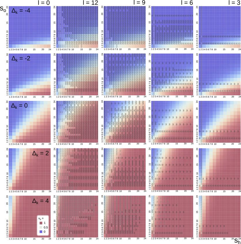
Here we focus on the stochastic dynamics of a particular, highly popular franchise of gamebooks,
the Fighting Fantasy (FF) series [Green, 2014]. This series, spanning over 50 adventure gamebooks
(exemplified by the famous first book in the series, ‘The Warlock of Firetop Mountain’ [Jackson and
Livingstone, 2002]), has sold over 20 million copies and given rise to a range of associated computer
games, board games, and apps, and is currently experiencing a dramatic resurgence in popularity [BBC,
2014, Österberg, 2008]. Outside of recreation, these adventures are used as pedagogical tools in the huge
industry of game design [Zagal and Lewis, 2015] and in teaching English as a foreign language [Philips,
1994].
    In FF, a player is assigned statistics (skill and stamina), dictating combat proficiency and en-
durance respectively. Opponents are also characterised by these combat statistics. Combat proceeds
iteratively through a series of ‘attack rounds’. In a given round, according to die rolls, the player may
draw, win or lose, respectively. These outcomes respectively have no effect, damage the opponent, and
damage the player. The player then has the option of using a limited resource (luck) to apply control
to the outcome of the round. This decision can be made dynamically, allowing the player to choose a
policy based on the current state of the system. However, each use of luck is a gamble [Maitra and
Sudderth, 2012, Dubins and Savage, 1965], where the probability of success depends on the current
level of the resource. If this gamble is successful, the player experiences a positive outcome (damage
to the opponent is amplified; damage to the player is weakened). If the gamble is unsuccessful, the
player experiences a negative outcome (damage to the opponent is weakened, damage to the player is
amplified). The optimal strategy for applying this control in a given state has yet to be found.
    This is a stochastic game [Shapley, 1953, Adlakha et al., 2015] played by one or two players (the
opponent usually has no agency to decide strategies) on a discrete state space with a finite horizon.
The game is Markovian: in the absence of special rules, the statistics of the player and opponent
uniquely determine a system state, and this state combined with a choice of policy uniquely determine
the transition probabilities to the next state. The problem of determining the optimal strategy is then a
Markov decision problem (MDP) [Bellman, 1957, Kallenberg, 2003]. In an MDP, a decision-maker must
choose a particular strategy for any given state of a system, which evolves according to Markovian
dynamics. In FF combat, the decision is always binary: given a state, whether or not to use the
dimishing resource of luck to attempt to influence the outcome of a given round.
    The study of stochastic games and puzzles is long established in operational research [Smith, 2007,
Bellman, 1965] and has led to several valuable and transferrable insights [Smith, 2007,Little et al., 1963].
Markov analysis, dynamic programming, and simulation have been recently used to explore strategies
and outcomes in a variety of games, sports, and TV challenges [Lee, 2012, Smith, 2007, Johnston, 2016,
Perea and Puerto, 2007, Percy, 2015, Clarke and Norman, 2003]. Specific analyses of popular one-
player recreational games with a stochastic element including Solitaire [Rabb, 1988, Kuykendall and
Mackenzie, 1999], Flip [Trick, 2001], Farmer Klaus and the Mouse [Campbell, 2002], Tetris [Kostreva
and Hartman, 2003], and The Weakest Link [Thomas, 2003]. These approaches typically aim to identify
the optimal strategy for a given state, and, in win/lose games, the overall probability of victory over
all possible instances of the game [Smith, 2007]. In stochastic dynamic games, counterintuitive optimal
strategies can be revealed through mathematical analysis, not least because ‘risking points is not the
same as risking the probability of winning’ [Neller and Presser, 2004].
    The FF system has some conceptual similarities with the well-studied recreational game Pig, and
other so-called ‘jeopardy race games’ [Neller and Presser, 2004, Smith, 2007], where die rolls are used
to build a score then a decision is made, based on the current state of the system, whether to gamble
further or not. Neller & Presser have used a value iteration approach to identify optimal strategies in
Pig and surveyed other similar games [Neller and Presser, 2004]. In FF combat, however, the player
has potential agency both over their effect on the opponent and the opponent’s effect on them. Further,
resource allocation in FF is a dynamic choice and also a gamble [Maitra and Sudderth, 2012, Dubins
and Savage, 1965], the success probability of which diminishes as more resource is allocated. The
probability of a negative outcome, as opposed to a positive one, therefore increases as more resource

                                                     2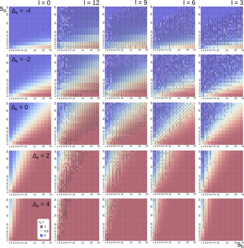
is used, providing an important ‘diminishing returns’ consideration in policy decision [Deckro and
Hebert, 2003]. In an applied context this could correspond to engaging in, for example, espionage and
counterespionage [Solan and Yariv, 2004], with increasing probability of negative outcomes with more
engagement in these covert activites.
    The optimal policy for allocating resource to improve a final success probability has been well
studied in the context of research and development (R&D) management [Heidenberger and Stummer,
1999, Baye and Hoppe, 2003, Canbolat et al., 2012, Gerchak and Parlar, 1999]. While policies in this
field are often described as ‘static’, where an initial ‘up-front’ decision is made and not updated over
time, dynamic policy choices allowing updated decisions to be made based on the state of the system
(including the progress of competitors) have also been examined [Blanning, 1981, Hopp, 1987, Posner
and Zuckerman, 1990]. Rent-seeking ‘contest’ models [Clark and Riis, 1998] also describe properties of
the victory probability as a function of an initial outlay from players. The ‘winner takes all’ R&D model
of Canbolat et al., where the first player to complete development receives all the available payoff, and
players allocate resource towards this goal [Canbolat et al., 2012], bears some similarity to the outcomes
of the FF system. The model of Canbolat et al. did not allow dynamic allocation based on the current
system state, but did allow a fixed cost to be spread over a time horizon, and computed Nash equilibria
in a variety of cases under this model.
    A connected branch of the literature considers how to allocate scarce resource to achieve an op-
timal defensive outcome [Golany et al., 2015, Valenzuela et al., 2015], a pertinent question both for
human [Golany et al., 2009] and animal [Clark and Harvell, 1992] societies. Both optimisation and
Nash equilibrium approaches are used in these contexts to identify solutions to the resource allocation
problem under different structures [Golany et al., 2015,Valenzuela et al., 2015]. The FF system has such
a defensive component, but the same resource can also be employed offensively, and as above takes the
unusual form of a gamble with a diminishing success probability.
    We will follow the philosophy of these optimisation approaches to identify the optimal strategy
for allocating resource to maximise victory probability from a given state in FF. We first describe the
system and provide solutions for victory probability in the case of no gambling and gambling according
to a simple policy. Next, to account for the influence of different gambling policies on the stochastic
dynamics of the game, we use a backwards-induction approach to solve the Bellman equation for the
system and optimise victory probability from any given state. We then identify simple heuristic rules
that approximate these optimised strategies and can be used in practise.

Game dynamics
Within an FF game, the player has nonnegative integer statistics called skill, stamina, and luck. skill
and luck are typically 6 12; stamina is typically 6 24, although these bounds are not required by our
analysis. In a given combat, the opponent will also have skill and stamina statistics. We label the
skill, stamina, and luck of the player (the ‘hero’) as kh , sh , and l respectively, and the opponent’s
skill and stamina as ko and so . Broadly, combat in the FF system involves a series of rounds, where
differences in skill between combatants influences how much stamina is lost in each round; when one
combatant’s stamina reaches zero or below, the combat is over and that combatant has lost. The player
may choose to use luck in any given round to influence the outcome of that round. More specifically,
combat proceeds through Algorithm 1.
   Algorithm 1. FF combat system.
  1. Roll two dice and add kh ; this is the player’s attack strength Ah .
  2. Roll two dice and add ko ; this is the opponent’s attack strength Ao .
  3. If Ah = Ao , this attack round is a draw. Go to 6.
  4. If Ah > Ao , the player has won this attack round. Make decision whether to use luck.
       (a) If yes, roll two dice to obtain r. If r 6 l, set so = so − 4. If r > l, set so = so − 1. For either
           outcome, set l = l − 1. Go to 6.

                                                      3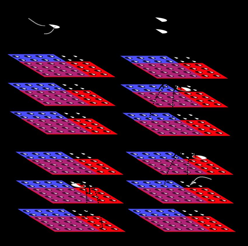
(b) If no, set so = so − 2. Go to 6.
   5. If Ah < Ao , the opponent has won this attack round. Make decision whether to use luck.
        (a) If yes, roll two dice to obtain r. If r 6 l, set sh = sh − 1. If r > l, set sh = sh − 3. For either
            outcome, set l = l − 1. Go to 6.
        (b) If no, set sh = sh − 2. Go to 6.
   6. If sh > 0 and so 6 0, the player has won; if so > 0 and sh 6 0, the opponent has won. Otherwise
      go to 1.
    It will readily be seen that these dynamics doubly bias battles in favour of the player. First, the
opponent has no opportunity to use luck to their benefit. Second, when used offensively (to support
an attack round that the player has won), the potential benefit (an additional 2 damage; Step 4a in
Algorithm 1) outweighs the potential detriment (a reduction of 1 damage; Step 5a in Algorithm 1).
When used defensively, this second bias is absent.
    We will retain the skill, stamina, luck terminology throughout this analysis. However, the con-
cepts here can readily be generalised. A player’s skill can be interpreted as their propensity to be
successful in any given competitive round. Their stamina can be interpreted as the amount of compet-
itive losses they can suffer before failure. luck is the resource that a player can dynamically allocate to
gamble on influencing the outcome of competitive rounds, that diminishes with use (so that the success
probability of the gamble also diminishes). For example, within the (counter)espionage analogy above,
skill could be perceived as a company’s level of information security, stamina its potential to lose
sensitive information before failure, and luck the resource that it can invest in (counter)espionage.

Analysis
In basic combat dynamics, skill does not change throughout a battle. The probabilities pw , pd , pl of
winning, drawing, an losing an attack round depend only on skill, and remain constant throughout
the battle. We therefore consider Pt (sh , so , l): the probability, at round t, of being in a state where the
player has stamina sh and luck l, and the opponent has stamina so . A discrete-time master equation
can readily be written down describing the dynamics above:

Pt+1 (sh , so , l) =
pw (1 − λ1 (sh , so + 2, l))Pt (sh , so + 2, l) + pw λ1 (sh , so + 4, l + 1)q(l + 1)Pt (sh , so + 4, l + 1)
 + pw λ1 (sh , so + 1, l + 1)(1 − q(l + 1))Pt (sh , so + 1, l + 1) + pl (1 − λ0 (sh + 2, so , l))Pt (sh + 2, so , l)
 + pl λ0 (sh + 3, so , l + 1)(1 − q(l + 1))Pt (sh + 3, so , l + 1) + pl λ0 (sh + 1, so , l + 1)q(l + 1)Pt (sh + 1, so , l + 1)
 − (1 − pd )Pt (sh , so , l).                                                                                          (1)

    Here, λi (sh , so , l) reflects the decision whether to use luck after a given attack round outcome i
(player loss i = 0 or player win i = 1), given the current state of the battle. This decision is free
for the player to choose. q(l) and (1 − q(l)) are respectively the probabilities of a successful and an
unsuccessful test against luck l. We proceed by first considering the case λ0 = λ1 = 0 (no use of luck).
We then consider a simplified case of constant luck, before using a dynamic programming approach
to address the full general dynamics.
    We are concerned with the victory probability vp with which the player is eventually victorious,
corresponding to a state where sh > 1 and so 6 0. We thus consider the ‘getting to a set’ outcome class
of this stochastic game [Maitra and Sudderth, 2012], corresponding to a ‘winner takes all’ race [Canbolat
et al., 2012]. We start with the probability of winning, drawing, or losing a given round. Let kh be the
player’s skill and ko be the opponent’s skill. Let D1 , ..., D4 be random variables drawn from a discrete
uniform distribution on [1, 6], and X = D1 + D2 − D3 − D4 . Let ∆k = kh − ko . Then, the probabilities of

                                                            4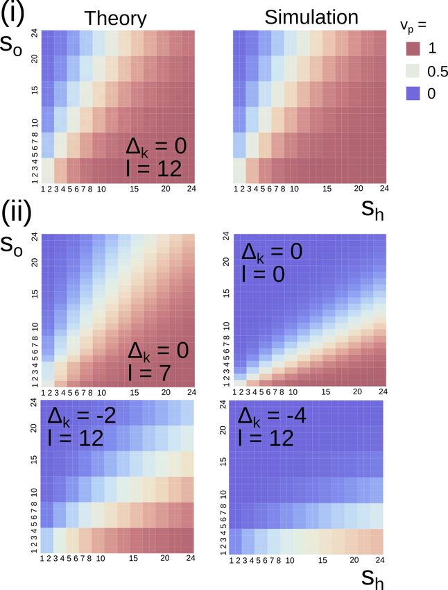
win, draw, and loss events correspond respectively to pw = P(X + ∆k > 0), pd = P(X + ∆k = 0), pl =
P(X + ∆k < 0).
    X is a discrete distribution on [−10, 10]. The point density       PP(X =i)       is proportional to the (i + 10)th
                                                                                     n
                                                                                                                         {1,
                                                                           5      j                                  1
sextinomial coefficient, defined via the generating function               j=0 x       , for n = 5 (specific values 1296
4, 10, 20, 35, 56, 80, 104, 125, 140, 146, 140, 125, 104, 80, 56, 35, 20, 10, 4, 1}; OEIS sequence A063260 [OEIS, 2019]).
Hence

                                                               X
                                                               10
                                             pw (∆k ) =                 P(X = j)                                    (2)
                                                           j=−∆k +1

                                             pd (∆k ) = P(X = −∆k )                                                 (3)
                                                            X
                                                           −∆k −1

                                              pl (∆k ) =              P(X = j)                                      (4)
                                                              j=−10

Dynamics without luck-based control
We first consider the straightforward case where the player employs no strategy, never electing to use
luck. We can then ignore l and consider steps through the (sh , so ) stamina space, which form a
discrete-time Markov chain. Eqn. 1 then becomes

              Pt+1 (sh , so , l) = pw Pt (sh , so + 2, l) + pl Pt (sh + 2, so , l) − (1 − pd )Pt (sh , so , l).     (5)

    We can consider a combinatorial approach based on ‘game histories’ describing steps moving
through this space [Maitra and Sudderth, 2012]. Here a game history is a string from the alphabet
{W, D, L}, with the character at a given position i corresponding to respectively to a win, draw, loss
in round i. We aim to enumerate the number of possible game histories that correspond to a given
outcome, and assign each a probability.
    We write w, d, l for the character counts of W, D, L in a given game history. A victorious game must
always end in W. Consider the string describing a game history omitting this final W. First leaving out
Ds, we have (w − 1) Ws and l Ls that can be arranged in any order. We therefore have n(w, l) = w−1+ll
possible strings, each of length w − 1 + l. For completeness, we can then place any number d of Ds
within these strings, obtaining

                                               w−1+l w−1+l+d
                                 n(w, l, d) =                             .                           (6)
                                                  l               d
   Write σh = bsh /2c and σo = bso /2c, describing the number of rounds each character can lose before
dying. Then, for a player victory, w = σo and l 6 σh − 1. d can take any nonnegative integer value.
The appearance of each character in a game string is accompanied by a multiplicative factor of the
corresponding probability, so we obtain
                                           σX    ∞
                                            h −1 X
                                                               w−1+l w−1+l+d
                             vp =   pσ
                                     w
                                       o
                                                     pll pd
                                                          d                   ,                                     (7)
                                                                 l      d
                                           l=0 d=0

   where the probability associated with the final W character has now also been included. After some
algebra, and writing ρw = pw /(1 − pd ) and ρl = pl /(1 − pd ), this expression becomes

                                                                                                       !
                                                            σh + σo − 1
   vp = pσ
         w (pl + pw )
           o          −σo
                               ρ−σ
                                w
                                   o
                                     − pσ h
                                        l (pl + pw )
                                                     −σh
                                                         ×               2 F1 (1, σh + σo , σh + 1, ρl )            (8)
                                                                σh

                                                                5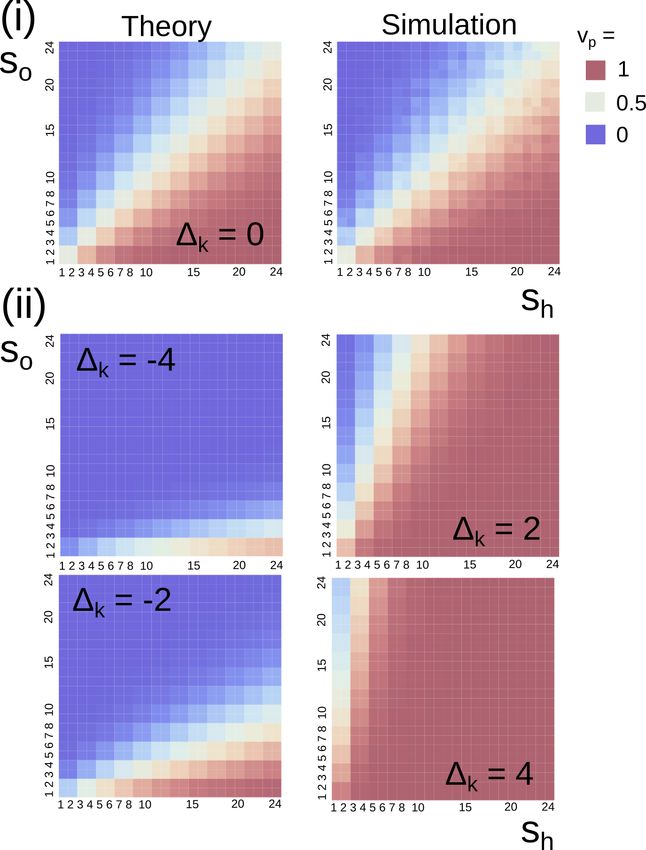
Figure 1: Victory probability in the absence of luck-based strategy. (i) Comparison of predicted victory probability vp
from Eqn. 8 with stochastic simulation. (ii) vp behaviour as skill difference ∆k changes.

    Eqn. 8 is compared with the result of stochastic simulation in Fig. 1, and shown for various skill
differences ∆k and (sh , so ) initial conditions. Intuitively, more favourable ∆k > 0 increase vp and less
favourable ∆k < 0 decrease vp for any given state, and discrepancies between starting sh and so also
influence eventual vp . A pronounced s (mod 2) structure is observed, as in the absence of luck, s = 2n
is functionally equivalent to s = 2n − 1 for integer n. For lower initial staminas, vp distributions
become more sharply peaked with s values, as fewer events are required for an eventual outcome.

Analytic dynamics with simplified luck-based control
To increase the probability of victory beyond the basic case in Eqn. 8, the player can elect to use luck in
any given round. We will first demonstrate that the above history-counting analysis can obtain analytic
results when applied to a simplified situation when luck is not depleted by use, so that the only limit
on its employment is its initial level [Blanning, 1981]. We then employ a dynamic programming scheme
to analyse the more involved general case.
    First consider the case where luck is only used offensively (step 4a in Algorithm 1), and is used
in every successful attack round. For now, ignore losses and draws. Then every game history consists
of As and Bs, where A is a successful offensive use of luck and B is an unsuccessful offensive use of
luck.
    Consider the game histories that lead to the opponent losing exactly n stamina points before the
final victorious round. There are bn/4c + 1 string lengths that can achieve this, which are L = n − 3k,
where k runs from 0 to bn/3c. The strings with a given k involve n − 4k failures and k successes.
    If we make the simplifying assumption that luck is not depleted with use, every outcome of a luck
test has the same success probability q(l) = q. Then the problem is simplified to finding the number of
ways of arranging k As and (n − 4k) Bs for each possible string:

                                                             6
(n − 3k)!
N(k) = (9)
k!(n − 4k)!
Now, for every string with a given k, with corresponding string length n − 3k, we can place l Ls
and d Ds as before, giving
(n − 3k)! n − 3k + l n − 3k + l + d
N(k; n, l, d) = . (10)
k!(n − 4k)! l d
The complete history involves a final victorious round. For now we will write the probability of this
event as pf , then the probability associated with this set of histories is
(n − 3k)! k n − 3k + l d n − 3k + l + d
P(k; n, l, d, pf ) = pf q (1 − q)n−4k pll pd (11)
k!(n − 4k)! l d
P h −1 P∞
and, as P(k; n, pf ) = σ
l=0 d=0 P(k; n, l, d, pf ),
1
P(k; n, pf ) =pf (1 − pd )3k−n−2−σh (pw − pw q)n−4k (pw q)k ρ−n−1 (n − 3k)!
k!(n − 4k)!
σh +1 3k σh n n − 3k + σh
× (1 − pd ) ρ + pl (pl + pd − 1)ρ 2 F1 (1, 1 − 3k + n + σh , 1 + σh , pl /(1 − pd ))
σh
(12)
where ρ = (pd + pl − 1)/(pd − 1). Hence
X
n/3
Pn (n, pf ) = P(k; n, pf ) (13)
k=0
Now consider the different forms that the final victorious round can take. The opponent’s stamina
can be reduced to 4 followed by an A, 3 followed by A, 2 followed by A, or 1 followed by A or B. If we
write P(m; X) for the probability of reducing the opponent’s stamina to m then finishing with event X,
vp = P(4; A) + P(3; A) + P(2; A) + P(1; A) + P(1; B) (14)
hence
vp = Pn (so − 4, q) + Pn (so − 3, q) + Pn (so − 2, q) + Pn (so − 1, q) + Pn (so − 1, (1 − q)). (15)
Fig. 2(i) compares Eqn. 15 and stochastic simulation, and shows that use of luck can dramatically
increase victory probability in a range of circumstances. Similar expressions can be derived for the
defensive case, where luck is solely used when a round is lost, and with some relaxations on the
structure of the sums involved the case where luck is not used in every round can also be considered.
Clearly, for constant luck, the optimal strategy is to always use luck when the expected outcome
is positive, and never when it is negative. The expected outcomes for offensive and defensive strategies
can readily be computed. For offensive use, the expected damage dealt when using luck is
hdi = 1 × (1 − q) + 4 × q (16)
In the absence of luck, d = 2 damage is dealt, so the expected outcome using luck is beneficial if
hdi > 2. We therefore obtain q > 31 as the criterion for employing luck. For comparison, the probability
of scoring 6 or under on two dice is q(6) = 0.417 and the probability of scoring 5 or under on two dice
is q(5) = 0.278.
7For defensive use, the expected damage received when using luck in an attack round is
hdi = 1 × q + 3 × (1 − q) (17)
In the absence of luck, d = 2 damage is taken, and we thus now obtain q > 12 as our criterion. For
comparison, the probability of scoring 7 or under on two dice is q(7) = 0.583.
The counting-based analyses above assume that luck stays constant. The dynamics of the game
actually lead to luck diminishing every time is it is used. Instead of the outcome of a luck test being
a constant q, it now becomes a function of how many tests have occurred previously.
To explore this situation, consider the above case where luck is always used offensively and never
defensively. Describe a given string of luck outcomes as an ordered set V of indices labelling where in
a string successes occur. For example, the string of length L = 5 with V = 2, 4 would be BABAB. Let
V 0 = Vc \ {1, ..., L}. Then
Y Y
P(V) = q(i) (1 − q(i)) (18)
i∈V i∈V 0
where q(i) is the probability of success on the ith luck test.
As above, for a given k, L = n − 3k, and we let S(k) be the set of ordered sets with k different
elements between 1 and n − 3k. Then the probability of a given string of As and Bs arising is
X
n/3
X Y Y
P(n) = q(i) (1 − q(i)) (19)
k=0 V∈S(k) i∈V i∈V 0
We can no longer use the simple counting argument in Eqn. 11 to compute the probabilities of
each history, because each probability now depends on the specific structure of the history. It will be
possible to enumerate these histories exhaustively but the analysis rapidly expands beyond the point
of useful interpretation, so we turn to dynamic programming to investigate the system’s behaviour.
Stochastic optimal control with dynamic programming
In a game with a given ∆k , we characterise every state of the system with a tuple S = {sh , so , l, O}
where O is the outcome (win or loss) of the current attack round. The question is, given a state, should
the player elect to use luck or not?
A common approach to identify the optimal strategy for a Markov decision problem in a discrete
state space is to use the Bellman equation [Bellman, 1957, Kirk, 2012], which in our case is simply
X
!
vp (S) = max Pa (S, S 0 )vp (S 0 ) . (20)
a
S0
Here, a is a strategy dictating what action to take in state S, Pa (S, S 0 ) is the probability under
strategy a of the transition from state S to state S 0 , and vp (S) is the probability-to-victory of state S.
The joint problem is to compute the optimal vp , and the strategy a that maximises it, for all states. To
do so, we employ a dynamic programming approach of backward induction [Bellman, 1957], starting
from states where vp is known and computing backwards through potential precursor states.
The dynamic programming approach first assigns a probability-to-victory vp for termination states
(Fig. 3(i)). For all ‘defeat’ states with sh 6 0, so > 0, we set vp = 0; for all ‘victory’ states with
so 6 0, sh > 0, set vp = 1 (states where both sh 6 0 and so 6 0 are inaccessible). We then iteratively
consider all states in the system where vp is fully determined for a loss outcome from the current round
(Fig. 3(ii)), and similarly for a win outcome (Fig. 3(iii)).
For states involving a loss outcome, we compute two probability propagators. The first corresponds
to the strategy where the player elects to use luck, and is of magnitude
8Figure 2: Victory probability with constant luck employed offensively. (i) Eqn. 15 compared to stochastic simulation. (ii)
Constant luck outcomes for intermediate and low luck, and for high luck mitigating low ∆k values.
X
py = Py (S, S 0 )vp (S 0 )
S0
= q(l)pl vp ({sh − 1, so , l − 1, 0}) + (1 − q(l))pl vp ({sh − 3, so , l − 1, 0})
+ q(l)pw vp ({sh − 1, so , l − 1, 1}) + (1 − q(l))pw vp ({sh − 3, so , l − 1, 1}) (21)
the second corresponds to the strategy where the player does not use luck, and is
X
pn = Pn (S, S 0 )vp (S 0 )
S0
= pl vp ({sh − 2, so , l, 0}) + pw vp ({sh − 2, so , l, 1}). (22)
When considering the probability-to-victory for a given state, we hence consider both the next
(sh , so , l) combination that a given event will lead to, and also both possible outcomes (win or loss)
from this state. For a given state, if py > pn , we record the optimal strategy as using luck and record
vp = py ; otherwise we record the optimal strategy as not to use luck and record vp = pn . In practise
we replace py > pn with the condition py > (1 + 10−10 )pn to avoid numerical artefacts, thus requiring
that the use of luck has a relative advantage to vp above 10−10 .
We do the same for states involving a win outcome from this round, where the two probability
propagators are now
py = q(l)pl vp ({sh , so − 4, l − 1, 0}) + (1 − q(l))pl vp ({sh , so − 1, l − 1, 0})
+ q(l)pw vp ({sh , so − 4, l − 1, 1}) + (1 − q(l))pw vp ({sh , so − 1, l − 1, 1}); (23)
9Figure 3: Dynamic programming scheme. The discrete state space of the game is represented by horizontal (sh ) and
vertical (so ) axes, layers (l) and a binary outcome at each position (O). (i) First, vp = 0 is assigned to states corresponding to
loss (sh 6 0, blue) and vp = 1 is assigned to states corresponding to victory (so 6 0, red). Then, iteratively, all states where
all outcomes have an assigned vp are considered. (ii) Considering outcomes after a loss in the current state (here, 1, 1, l, 0,
highlighted red). The probability-to-victory for a ‘no’ strategy corresponds to the solid line; the probability-to-victory for
a ‘yes’ strategy consists of contributions from both dashed lines (both outcomes from a luck test). (iii) Same process for a
win outcome from the current state. (iv) Now the previous node has characterised probabilities-to-victory for both loss and
win outcomes, a next iteration of nodes can be considered. Now, the probability-to-victory from a ‘yes’ strategy has a term
corresponding to the potential outcomes from the previously characterised node.
10and
pn = pl vp ({sh , so − 2, l, 0}) + pw vp ({sh , so − 2, l, 1}). (24)
Each new pair of states for which the optimal vp is calculated opens up the opportunity to compute
vp for new pairs of states (Fig. 3(iv)). Eventually a vp and optimal strategy is computed for each
outcome, providing a full ‘roadmap’ of the optimal decision to make under any circumstance. This full
map is shown in Supplementary Fig. 6, with a subset of states shown in Fig. 4.
We find that a high luck score and judicious use of luck can dramatically enhance victory proba-
bility against some opponents. As an extreme example, with a skill detriment of ∆k = −9, sh = 2, so =
23, l = 12, use of luck increased victory probability by a factor of 1018 , albeit to a mere 2.3 × 10⁻¹⁹ .
On more reasonable scales, with a skill detriment of ∆k = −4, sh = 22, so = 19, l = 12, use of luck
increased victory probability 1159-fold, from 9.8 × 10⁻⁶ to 0.011 (the highest fold increase with the final
probability greater than 0.01). With a skill detriment of ∆k = −2, sh = 22, so = 21, l = 12, use of
luck increased victory probability 21-fold, from 0.010 to 0.22 (the highest fold increase with the initial
probability greater than 0.01). Using encounters that appear in the FF universe [Gascoigne, 1985], for
a player with maximum statistics kh = 12, sh = 24, l = 12, optimal use of luck makes victory against
an adult White Dragon (ko = 15, so = 22) merely quite unlikely (vp = 0.046) rather than implausible
(vp = 4.4 × 10⁻⁴ ), and victory against a Hell Demon (ko = 14, so = 12) fairly straightforward (vp = 0.78)
rather than unlikely (vp = 0.28).
Structure of optimal policy space
There is substantial similarity in optimal policy choice between several regions of state space. For
large skill deficiencies ∆k 6 −6 (low probability of victory) the distribution of optimal strategies in
stamina space is the same for a given l for all ∆k . For higher l, this similarity continues to higher
∆k ; for l = 12, only 5 points in stamina space have different optimal strategies for ∆k = −9 and
∆k = −4. At more reasonable victory probabilities, a moderate transition is apparent between l = 6
and l = 5, where the number of points in stamina space where the optimal strategy involves using
luck decreases noticeably. This reflects the lower expected advantage for l = 5 (Eqns. 16-17).
The interplay of several general strategies is observed in the optimal structures. First note that
ds/4e gives the number of hits required for defeat if a hit takes 4 stamina points (a successful offensive
luck test) and ds/2e gives the number of hits required for defeat in the absence of strategy. These
scales partition stamina space by the number of rounds required for a given outcome and hence
dictate several of the ‘banded’ structures observable in strategy structure. For example, at sh = 2, it is
very advantageous for the player to attempt to mitigate the effect of losing another round. Almost all
circumstances display a band of defensive optimal strategy at sh = 2.
At so = 3, a successful offensive luck test is very advantageous (immediate victory). An unsuc-
cessful offensive test, leading to so = 2, is not disadvantageous to the same extent: we still need exactly
one successful attack round without luck, as we would if we had not used luck and achieved so = 1
instead. A strip of strategy 3 (or strategy 1) at so = 3 is thus the next most robustly observed feature,
disappearing only when victory probability is already overwhelmingly high. Many other structural
features result from a tradeoff between conserving luck and increasing the probability of encountering
this advantageous region. An illustration of the broad layout of optimal strategies is shown in Fig. 5; a
more fine-grained analysis is provided in the Appendix.
Simulated dynamics with heuristic luck strategies
While the dynamic programming approach above gives the optimal strategy for any circumstance,
the detailed information involved does not lend itself to easy memorisation. As in Smith’s discussion
11Figure 4: Optimal strategies and victory probabilities throughout state space. The optimal strategy at a given state is
given by the number at the corresponding point (1 – use luck regardless of the outcome of this round; 2 – use luck if this
round is lost; 3 – use luck if this round is won). No number means that the optimal strategy is not to employ luck regardless
of outcome. Colour gives victory probability vp .
12Figure 5: Summary of optimal strategies and victory probabilities throughout state space. Arrows depict regions where
the optimal policy depends on current available luck, including the general change in that region with decreasing luck.
Empty regions are those where avoiding the use of luck is the optimal policy. Other policies: (i) Hero stamina = 2: use luck
defensively (but see (iv), (v)); (ii) Opponent stamina 6 2: use luck defensively; (iii) Use luck offensively, particularly when
opponent stamina (mod 4) = 3; (iv) Use luck offensively and defensively; (v) Use luck defensively, and offensively if luck
is high and opponent stamina (mod 4) = 3 or 0.
of solitaire, ‘the curse of dimensionality applies for the state description, and most wise players use
heuristics’ [Smith, 2007]. We therefore consider, in addition to the semi-quantitative summary in Fig.
5, coarse-grained quantitative ‘strategies’ that, rather than specifying an action for each branch of the
possible tree of circumstances, use a heuristic rule that is applied in all circumstances.
Among the simplest strategies are ‘open-loop’ rules, where the current state of the player’s and the
opponent’s stamina does not inform the choice of whether to use luck. We may also consider ‘feed-
back’ rules, where the current state of staminas informs this choice. We parameterise luck strategies
by a threshold τ; luck will only be used if the player’s current luck score is greater than or equal to τ.
We consider the following luck strategies:
0. Never use luck (λ0 = λ1 = 0 as above);
1. Use luck in every non-draw round (i.e. to both ameliorate damage and enhance hits, λ0 = λ1 =
Θ(l > τ));
2. Use luck defensively (i.e. only to ameliorate damage, λ1 = 0, λ0 = Θ(l > τ));
3. Use luck offensively (i.e. only to enhance hits, λ0 = 0, λ1 = Θ(l > τ));
4. Use luck defensively if l > τ and sh < 6;
5. Use luck offensively if l > τ and so > 6;
6. Use luck if l > τ and sh < 6;
7. Use luck if l > τ and sh < 4;
8. Use luck if l > τ and sh < so .
Strategy 0 is the trivial absence of luck use; strategies 1-3 are ‘open-loop’ and 4-8 are ‘feedback’.
Strategies 2 and 4 are defensive; strategies 3 and 5 are offensive; strategies 1, 6, 7, 8 are both offensive
and defensive.
The analytic structure determined above is largely visible in the simulation results (Supplementary
Fig. 7). The main differences arise from the construction that the same strategy is retained throughout
combat in the simulation study. For low ∆k , high l, the favouring of strategy 3 except at low sh
(strategy 1) and so < 2 (strategy 2) is clear. At low sh , some feedback strategies gain traction: for
example, strategy 8, which is identical to strategy 1 when l is high and sh < so , but avoids depleting
luck if ever sh > so , is more conservative than always using strategy 1. Similarly, strategy 5 provides
a feedback alternative to strategy 3, using luck only at so > 6, which is favoured at intermediate
l and high so where it is beneficial to preserve luck. These feedback-controlled options mimic the
state-specific application of strategy found in the optimal cases in Fig. 4.
13Decreasing l introduces the sparsification of the strategy 3 regions – an effect which, as with the
analysis, is more pronounced at higher ∆k . In simulations, at higher ∆k , the increasingly small relative
increases in victory probability mean that several regions do not display substantial advantages to using
strategy. However, at moderate to positive ∆k , the increased takeover of strategy 2 is observed for high
so , low sh . Strategy 4, a more conservative feedback version of strategy 2, also experiences support in
these regions, competing with strategy 2 particularly in bands where sh (mod 2) = 0, as described in
the analytic case. The above banded structures of strategies 2 and 3, and the ubiquitous strategy 2 (or
equivalent) at sh = 2, are also observed for intermediate l.
Under these simplified rulesets, what is the optimal threshold τ above which we should use luck?
Straightforward application of Eqns. 16-17 are supported by simulation results (Supplementary Fig. 8),
where the probability that a given τ appears in the highest vp strategy peaked at τ = 6 for strategy 1
and τ = 5 for strategy 3.
A heuristic approach harnessing these insights, at the broad level of Fig. 5, might be as follows.
Employ strategy 3 (offensive luck use), unless: (i) initial luck is high or so is low, in which case strategy
1 (unconditional luck use); (ii) kh > ko and (i) is not true, in which case strategy 2 (defensive luck
use); or (iii) ko > kh and so 6 2 and (i) is not true, in which case strategy 2 (defensive luck use). At
the next level of detail, feedback control in the form of strategies 4-8 may be beneficial in some cases,
notably when luck depletion is likely to become an issue; regions where this is likely to be the case
can be read off from Supplementary Fig. 7. Finally, the optimal strategy for any given state can be read
off from Supplementary Fig. 6.
Discussion
We have examined the probability of victory in an iterated, probabilistic game that plays a central role
in a well-known and widespread interactive fiction series. The game can be played with or without
‘strategy’, here manifest by the consumption of a limited resource to probabilistically influence the
outcome of each round.
Several interesting features of the FF combat system make it potentially noteworthy with respect to
similar systems [Canbolat et al., 2012, Neller and Presser, 2004, Smith, 2007]. The allocation of resource
is dynamic and depends on system state [Blanning, 1981, Hopp, 1987, Posner and Zuckerman, 1990].
The use of resource can both increase the probability of a positive outcome for the player, or a negative
outcome for the opponent. Use of this resource does not guarantee a positive outcome: its use is a
gamble [Maitra and Sudderth, 2012, Dubins and Savage, 1965] that may negatively affect the player.
The probability of this negative effect increases as more resource is used, providing an important
consideration in the decision of whether to invoke this policy in the face of ‘diminishing returns’
[Deckro and Hebert, 2003].
The fact that gambles are dynamically used to influence iterated stochastic dynamics complicates
the analysis of the game. To employ dynamic programming, state space was labelled both by the
current statistics of the players and by the outcome of the current stochastic round. The policy decision
of whether to gamble thus depends both on current statistics and the outcome of a round.
This analysis reveals several structural properties of the system that are not specific to the FF context
of this study. The case of a limited resource being gambled against to both amplify successes and
mitigate failures (with the probability of a positive outcome diminishing as resource is used) bears
some resemblance to, for example, a conceptual picture of espionage and counterespionage [Solan and
Yariv, 2004]. For example, resource could be allocated to covert operations with some probability of
amplifying thefts and mitigating losses of information, with increased probability of negative outcomes
due to discovery as these covert activites are employed more. Our analysis then reveals the strategies
to be employed in different scenarios of information security (skill) and robustness to information loss
(stamina).
In the absence of strategy, we find a closed-form expression for victory probability that takes an
14intuitive form. When strategy is included, dramatic increases in victory probability are found. The
strong advantages provided by successful use of resource towards the ‘endgame’, where a successful
gamble will produce instant victory or avoid instant defeat, shapes the structure of the optimal policy
landscape. When little resource is available, complex structures emerge in the optimal landscape that
depend on the tradeoff between using resource in the current state or ‘saving’ it in case of a more
beneficial state later (‘risking points is not the same as risking the probability of winning’ [Neller and
Presser, 2004]). When default victory is unlikely, using resource to reinforce rare success probabilities
is a favoured strategy; when default victory is likely, using resource to mitigate rare loss probabilities
is favoured. The specific optimal policy in a given state is solved and can be reasonably approximated
by more heuristic strategies [Smith, 2007]. Interestingly, there is little performance loss when these
heuristics are ‘open-loop’, in the sense that policy choice only depends on a round’s outcome and
coarsely on the amount of current resource. ‘Feedback’ strategies additionally based on the statistics of
the two players did not provide a substantial advantage as long as endgame dynamics were covered.
Numerous FF gamebooks embellish the basic combat system, where weapons, armour, and other
circumstances led to different stamina costs or different rules. In the notoriously hard ‘Crypt of the
Sorcerer’ [Livingstone, 1987], if the final opponent (with ko = 12) wins two successive rounds the player
is instantly killed, altering the Markovian nature of the combat system (and substantially decreasing
victory probability). A simulation study [Fitti, 2016], while not employing an optimised luck strategy,
estimated a 95% probability of this instant death occurring (and a 0.11% probability of overall victory
through the book). Further expansion of this analysis will generalise the potential rulesets, and hence
allow the identification of optimal strategies in more situations.
Another route for expansion involves optimising victory probability while preserving some statis-
tics, for example enforcing that sh > s∗ or l > l∗ at victory, so that some resource is retained for the rest
of the adventure after this combat. Such constraints could readily be incorporated through an initial
reallocating vp over system states in the dynamic programming approach (Fig. 3(i)), or by expanding
the definition of the score being optimised to include some measure of desired retention in addition to
vp .
In an era of artificial intelligence approaches providing effective but essentially uninterpretable
strategies for complex games [Campbell et al., 2002, Lee et al., 2016, Gibney, 2016], more targetted anal-
yses still have the potential to inform more deeply about the mechanisms involved in these strategies.
Further, mechanistic understanding makes successful strategies readily available and simple to im-
plement in the absence of computational resource. We hope that this increased interpretability and
accessibility both contribute to the demonstration of the general power of these approaches, and help
improve the experience of some of the millions of FF players worldwide.
Acknowledgments
The author is grateful to Steve Jackson, Ian Livingstone, and the many other FF authors for creating
this system and the associated worlds. The author also thanks Daniel Gibbs and Ellen Røyrvik for
productive discussions.
References
[Adlakha et al., 2015] Adlakha, S., Johari, R., and Weintraub, G. Y. (2015). Equilibria of dynamic games
with many players: Existence, approximation, and market structure. Journal of Economic Theory,
156:269–316.
[Baye and Hoppe, 2003] Baye, M. R. and Hoppe, H. C. (2003). The strategic equivalence of rent-seeking,
innovation, and patent-race games. Games and economic behavior, 44(2):217–226.
15[BBC, 2014] BBC (2014). Retrieved from https://www.bbc.co.uk/news/magazine-28865399, june
2019.
[Bellman, 1957] Bellman, R. (1957). A Markovian decision process. Journal of Mathematics and Mechanics,
pages 679–684.
[Bellman, 1965] Bellman, R. (1965). On the application of dynamic programing to the determination of
optimal play in chess and checkers. Proceedings of the National Academy of Sciences of the United States
of America, 53(2):244.
[Blanning, 1981] Blanning, R. W. (1981). Variable-base budgeting for r&d. Management Science,
27(5):547–558.
[Campbell et al., 2002] Campbell, M., Hoane Jr, A. J., and Hsu, F.-h. (2002). Deep blue. Artificial intelli-
gence, 134(1-2):57–83.
[Campbell, 2002] Campbell, P. J. (2002). Farmer klaus and the mouse. The UMAP Journal, 23(2):121–134.
[Canbolat et al., 2012] Canbolat, P. G., Golany, B., Mund, I., and Rothblum, U. G. (2012). A stochastic
competitive r&d race where winner takes all. Operations Research, 60(3):700–715.
[Clark and Harvell, 1992] Clark, C. W. and Harvell, C. D. (1992). Inducible defenses and the allocation
of resources: a minimal model. The American Naturalist, 139(3):521–539.
[Clark and Riis, 1998] Clark, D. J. and Riis, C. (1998). Contest success functions: an extension. Economic
Theory, 11(1):201–204.
[Clarke and Norman, 2003] Clarke, S. R. and Norman, J. M. (2003). Dynamic programming in cricket:
Choosing a night watchman. Journal of the Operational Research Society, 54(8):838–845.
[Costikyan, 2007] Costikyan, G. (2007). Games, storytelling, and breaking the string. Second Person:
Roleplaying and Story in Playable Media, pages 5–14.
[Deckro and Hebert, 2003] Deckro, R. F. and Hebert, J. E. (2003). Modeling diminishing returns in
project resource planning. Computers & industrial engineering, 44(1):19–33.
[Dubins and Savage, 1965] Dubins, L. E. and Savage, L. J. (1965). Inequalities for stochastic processes: How
to gamble if you must. Dover Publications.
[Fitti, 2016] Fitti (2016). Retrieved from https://www.youtube.com/watch?v=-kMwT8QWZnw, june 2019.
[Gascoigne, 1985] Gascoigne, M. (1985). Out of the Pit. Puffin Books.
[Gerchak and Parlar, 1999] Gerchak, Y. and Parlar, M. (1999). Allocating resources to research and
development projects in a competitive environment. Iie Transactions, 31(9):827–834.
[Gibney, 2016] Gibney, E. (2016). Google AI algorithm masters ancient game of Go. Nature News,
529(7587):445.
[Golany et al., 2015] Golany, B., Goldberg, N., and Rothblum, U. G. (2015). Allocating multiple defen-
sive resources in a zero-sum game setting. Annals of Operations Research, 225(1):91–109.
[Golany et al., 2009] Golany, B., Kaplan, E. H., Marmur, A., and Rothblum, U. G. (2009). Nature plays
with dice–terrorists do not: Allocating resources to counter strategic versus probabilistic risks. Euro-
pean Journal of Operational Research, 192(1):198–208.
[Green, 2014] Green, J. (2014). You are the Hero. Snowbooks Ltd.
16[Gygax and Arneson, 1974] Gygax, G. and Arneson, D. (1974). Dungeons and dragons, volume 19. Tac-
tical Studies Rules Lake Geneva, WI.
[Heidenberger and Stummer, 1999] Heidenberger, K. and Stummer, C. (1999). Research and devel-
opment project selection and resource allocation: a review of quantitative modelling approaches.
International Journal of Management Reviews, 1(2):197–224.
[Hopp, 1987] Hopp, W. J. (1987). A sequential model of r&d investment over an unbounded time
horizon. Management Science, 33(4):500–508.
[Jackson and Livingstone, 2002] Jackson, S. and Livingstone, I. (2002). The Warlock of Firetop Mountain.
Wizard Books.
[Johnston, 2016] Johnston, I. G. (2016). Endless love: On the termination of a playground number game.
Recreational Mathematics Magazine, 3(5):61–78.
[Kallenberg, 2003] Kallenberg, L. (2003). Finite state and action MDPs. In Handbook of Markov decision
processes, pages 21–87. Springer.
[Kirk, 2012] Kirk, D. E. (2012). Optimal control theory: an introduction. Courier Corporation.
[Kostreva and Hartman, 2003] Kostreva, M. M. and Hartman, R. (2003). Multiple objective solutions
for tetris. Journal of Recreational Mathematics, 32(3):214.
[Kuykendall and Mackenzie, 1999] Kuykendall, C. and Mackenzie, D. (1999). Analyzing solitaire. Sci-
ence, 283(5403):794–794.
[Lee et al., 2016] Lee, C.-S., Wang, M.-H., Yen, S.-J., Wei, T.-H., Wu, I.-C., Chou, P.-C., Chou, C.-H.,
Wang, M.-W., and Yan, T.-H. (2016). Human vs. computer go: Review and prospect [discussion
forum]. IEEE Computational intelligence magazine, 11(3):67–72.
[Lee, 2012] Lee, J. D. (2012). The Comparison of Strategies used in the game of RISK via Markovian
Analysis and Monte-Carlo Simulation. Technical Report AFIT/IOA/ENS/12-02, Air Force Inst of
Tech Wright-Patterson AFB OH Graduate School of Engineering and Management.
[Little et al., 1963] Little, J. D., Murty, K. G., Sweeney, D. W., and Karel, C. (1963). An algorithm for the
traveling salesman problem. Operations research, 11(6):972–989.
[Livingstone, 1987] Livingstone, I. (1987). Crypt of the Sorcerer. Puffin Books.
[Maitra and Sudderth, 2012] Maitra, A. P. and Sudderth, W. D. (2012). Discrete gambling and stochastic
games, volume 32. Springer Science & Business Media.
[Neller and Presser, 2004] Neller, T. W. and Presser, C. G. (2004). Optimal play of the dice game pig.
The UMAP Journal, 25(1).
[OEIS, 2019] OEIS (2019). The On-Line Encyclopedia of Integer Sequences, published electronically at
https://oeis.org.
[Österberg, 2008] Österberg, A. (2008). The Rise and Fall of the Gamebook. Re-
trieved from http: // www. outspaced. fightingfantasy. net/ Hosted/ Anders_ -_ The_ Rise_ and_
Fall_ of_ the_ Gamebook. pdf , June 2019.
[Percy, 2015] Percy, D. F. (2015). Strategy selection and outcome prediction in sport using dynamic
learning for stochastic processes. Journal of the Operational Research Society, 66(11):1840–1849.
17[Perea and Puerto, 2007] Perea, F. and Puerto, J. (2007). Dynamic programming analysis of the tv game
who wants to be a millionaire?. European Journal of Operational Research, 183(2):805–811.
[Philips, 1994] Philips, B. (1994). Role-playing games in the English as a Foreign Language Classroom.
Proceedings of the Tenth National Conferences on English Teaching and Learning in the Republic of China,
pages 624–648.
[Posner and Zuckerman, 1990] Posner, M. and Zuckerman, D. (1990). Optimal r&d programs in a
random environment. Journal of Applied Probability, 27(2):343–350.
[Rabb, 1988] Rabb, A. (1988). A probabilistic analysis of the game of solitaire. Undergraduate honors
thesis, Harvard University.
[Shapley, 1953] Shapley, L. S. (1953). Stochastic games. Proceedings of the national academy of sciences,
39(10):1095–1100.
[Smith, 2007] Smith, D. K. (2007). Dynamic programming and board games: A survey. European Journal
of Operational Research, 176(3):1299–1318.
[Solan and Yariv, 2004] Solan, E. and Yariv, L. (2004). Games with espionage. Games and Economic
Behavior, 47(1):172–199.
[Thomas, 2003] Thomas, L. (2003). The best banking strategy when playing the weakest link. Journal of
the Operational Research Society, 54(7):747–750.
[Trick, 2001] Trick, M. A. (2001). Building a better game through dynamic programming: A flip analy-
sis. INFORMS Transactions on Education, 2(1):50–58.
[Valenzuela et al., 2015] Valenzuela, M., Szidarovszky, F., and Rozenblit, J. (2015). A multiresolution
approach for optimal defense against random attacks. International Journal of Information Security,
14(1):61–72.
[Zagal and Lewis, 2015] Zagal, J. P. and Lewis, C. (2015). Fighting Fantasies: Authoring RPG Game-
books for Learning Game Writing and Design. Proceedings of the 2015 RPG Summit-DiGRA 2015
Conference: Diversity of Play.
18Appendix
Detailed structure of optimal policy space
Lower ∆k . In this regime, for sh = 2, there is a band of strategy 2, reflecting the fact that luck is best
spent attempting to avoid the fatality of a lost attack round. For certain so regions, strategy 3 is optimal.
For example, when l is low, strategy 3 appears when so = 3 or 4. Here, the probability of winning
an attack round is very low, so even a small chance of a successful luck test amplifying the outcome
to a killing blow is worth taking. These bands of strategy 3 propagate as l increases, occupying strips
between so = 3 and so = 4n. One sopp value is omitted from each band, at so = 2 + 4n. It will be
noticed that these values are those where, if luck is not employed, a successful round (so − 2) will
decrease dso /4e, whereas if luck is employed and is not successful (so − 1), that next band will not be
reached. When luck is a limited resource it does not pay to ‘spend’ it in these cases.
Where strategy 2 and 3 bands overlap, intuitively, strategy 1 appears, using luck for either outcome.
As l increases further (l > 8) other regions of stamina space display a preference for strategy 2,
reflecting the fact that substantial luck is now available relative to the likely number of remaining
attack rounds, so that is pays to invest luck defensively as well as offensively. As l increases further
still, the expanding regions of strategy 2 overlap more with existing strategy 3 regions, leading to an
expansion of strategy 1 in low sh regions.
Column-wise, beginning at ∆k = −6, some horizontal bands in the the strategy 3 region sparsify
into sh (mod 2) = 1 bands. This banding reflects the ubiquitous presence of strategy 2 when sh = 2,
to potentially defer the final fatal loss and allow one more attack round. If sh (mod 2) = 1, this region
will not be reached unless the player uses a (non-optimal) defensive strategy elsewhere, so luck can
be freely invested in offensive strategy. If sh (mod 2) = 0, the battle has some probability (high if ∆k is
low) of encountering the sh = 2 state, so there is an advantage to preserving luck for this circumstance.
Higher ∆k . Patterns of strategies 2-3 remains largely unchanged as ∆k increases, until the regions
of strategy 3 at lower l start to become sparsified, breaking up both row-wise and column-wise. Row-
wise breaks, as above, occur at so = 2 + 4n, so that low luck is not used if the outcome will not cross
a dso /4e band. Eventually these breaks are joined by others, so that for e.g. ∆k = −4, l = 4 strategy 3
only appears in bands of so = 3 + 4n. Here, a successful luck test shifts the system to the next dso /4e
band, while an unsuccessful luck test means that the next band can be reached with a successful attack
round without using luck. Column-wise, strategy 2 expands in sh (mod 2) = 0 bands at higher ∆k ,
and the ongoing sparsification of strategy 3 regions for low l as ∆k increases.
For higher l, as ∆k increases, the sparsification of strategy 3 regions occurs in tandem with an
expansion of strategy 2 regions. Strategy 2 becomes particularly dominant in high so , low sh regions.
Here, the player expects to win most attack rounds, and the emphasis shifts to minimising losses from
the rare attack rounds that the opponent wins, so that the player has time to win without their stamina
running out. A banded structure emerges (for example, ∆k = 2, l = 12) where for so (mod 4) 6 1
strategy 2 is favoured and for so (mod 4) > 2 strategies 1 and 3 are favoured. This structure emerges
because of the relatively strong advantage of a successful luck test at so = 3 and so = 4, leading
to immediate victory, and the propagating advantage of successful luck tests that lead to this region
(wherever so (mod 4) > 2). In the absence of this advantage (so (mod 4) 6 q), the best strategy is to
minimise damage from rare lost rounds until the advantageous bands are obtained by victories without
depleting luck.
At higher yet ∆k , victory is very likely, and the majority of stamina space for high l is dominated
by the defensive strategy 2 – minimising the impact of the rare attack rounds where the opponent wins.
At intermediate l, strategies 2 and 3 appear in banded formation, where defensive luck use is favoured
when sh is even, to increase the number of steps needed to reach sh = 0.
19You can also read