Creating a Field-Wide Forage Canopy Model Using UAVs and Photogrammetry Processing
←
→
Page content transcription
If your browser does not render page correctly, please read the page content below
remote sensing
Technical Note
Creating a Field-Wide Forage Canopy Model Using UAVs and
Photogrammetry Processing
Cameron Minch, Joseph Dvorak * , Josh Jackson and Stuart Tucker Sheffield

                                          Department of Biosystems and Agricultural Engineering, University of Kentucky, Lexington, KY 40546, USA;
                                          cameronlmagolan@uky.edu (C.M.); joshjackson@uky.edu (J.J.); st.sheffield@uky.edu (S.T.S.)
                                          * Correspondence: joe.dvorak@uky.edu

                                          Abstract: Alfalfa canopy structure reveals useful information for managing this forage crop, but
                                          manual measurements are impractical at field-scale. Photogrammetry processing with images from
                                          Unmanned Aerial Vehicles (UAVs) can create a field-wide three-dimensional model of the crop
                                          canopy. The goal of this study was to determine the appropriate flight parameters for the UAV
                                          that would enable reliable generation of canopy models at all stages of alfalfa growth. Flights were
                                          conducted over two separate fields on four different dates using three different flight parameters.
                                          This provided a total of 24 flights. The flight parameters considered were the following: 30 m
                                          altitude with 90◦ camera gimbal angle, 50 m altitude with 90◦ camera gimbal angle, and 50 m altitude
                                          with 75◦ camera gimbal angle. A total of 32 three-dimensional canopy models were created using
                                          photogrammetry. Images from each of the 24 flights were used to create 24 separate models and
                                images from multiple flights were combined to create an additional eight models. The models were

                                          analyzed based on Model Ground Sampling Distance (GSD), Model Root Mean Square Error (RMSE),
Citation: Minch, C.; Dvorak, J.;          and camera calibration difference. Of the 32 attempted models, 30 or 94% were judged acceptable.
Jackson, J.; Sheffield, S.T. Creating a   The models were then used to estimate alfalfa yield and the best yield estimates occurred with flights
Field-Wide Forage Canopy Model
                                          at a 50 m altitude with a 75◦ camera gimbal angle; therefore, these flight parameters are suggested
Using UAVs and Photogrammetry
                                          for the most consistent results.
Processing. Remote Sens. 2021, 13,
2487. https://doi.org/10.3390/
                                          Keywords: forage canopy; photogrammetry; three-dimensional model; UAV
rs13132487

Academic Editors: Mehdi Hosseini,
Ritvik Sahajpal, Hannah Kerner and
Magaly Koch                               1. Introduction
                                                Alfalfa was the third most valuable field crop in the United States in 2017 and 2018 [1,2].
Received: 9 April 2021                    However, unlike other top field crops, alfalfa is a forage primarily grown for its biomass.
Accepted: 18 June 2021                    As a perennial, multiple harvests per year are produced over multiple years. Alfalfa’s yield
Published: 25 June 2021                   in any given harvest is determined by the height and density of the plant canopy [3]. Addi-
                                          tionally, the nutritive value is a critical factor in the quality of the harvested biomass [4,5].
Publisher’s Note: MDPI stays neutral      In alfalfa, there is a tradeoff between nutritive value and yield [6]. As the plant matures and
with regard to jurisdictional claims in   grows taller, which increases yield, the concentration of less digestible components, such
published maps and institutional affil-   as lignin, increases and the nutritive value decreases [7,8]. The optimal relationship varies
iations.
                                          and is affected by location, enterprise management strategies, markets, anticipated end
                                          uses, weather, and climate factors unique to every farm and every harvest [9]. Furthermore,
                                          alfalfa stands weaken and thin over time and cannot be reseeded. Therefore, another
                                          unique decision in growing alfalfa is when to destroy the remaining stand and rotate into
Copyright: © 2021 by the authors.         other crops. Alfalfa producers need to be aware of the state of the crop to select harvest
Licensee MDPI, Basel, Switzerland.        times and crop rotation schedules that optimize the value to their enterprise [9]. All these
This article is an open access article    considerations are required on top of monitoring for diseases, weeds, and other pest issues
distributed under the terms and           in order to deploy appropriate mitigation strategies that are just as important in alfalfa as
conditions of the Creative Commons
                                          in any field crop. The structure of the alfalfa canopy is directly related to many important
Attribution (CC BY) license (https://
                                          production factors such as yield, quality, stand health, and pest control [10–12]. A three
creativecommons.org/licenses/by/
                                          dimensional (3D) model of the physical structure of the alfalfa canopy can be used to
4.0/).

Remote Sens. 2021, 13, 2487. https://doi.org/10.3390/rs13132487                                     https://www.mdpi.com/journal/remotesensing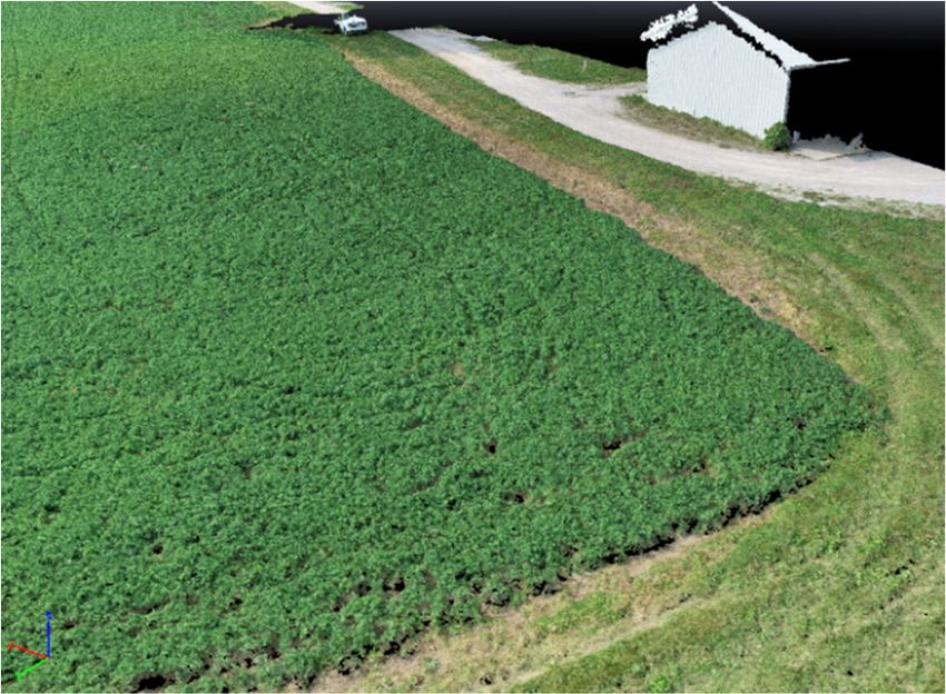
Remote Sens. 2021, 13, 2487                                                                                            2 of 15

                              determine the nutritive value and yield of an alfalfa crop while it is still growing in the
                              field [13].
                                    Unmanned Aerial Vehicles (UAVs) have gained much attention for their potential ap-
                              plication as rapid sensing platforms in agriculture. They have proven useful in monitoring
                              soybean disease [14], plant pests in vineyards [15], and crop condition in sorghum [16].
                              Furthermore, UAVs can also measure the phenotype of plants in breeding programs for
                              various crops from tomatoes [17], wheat [18], and sorghum [19]. Pre-harvest yield has been
                              estimated in cotton [20,21]. Sensors on the UAV platforms have also been used to estimate
                              the biomass of barley for fertilizer optimization [22] and the biomass of wheat for crop
                              monitoring and yield predictions [23,24].
                                    All of these studies used photogrammetry to combine the large number of visual or
                              hyperspectral images taken by the UAVs into a single output. In most cases, this was a two-
                              dimensional visual light and/or hyperspectral orthomosaic of the field. Photogrammetry
                              can also be used to create three dimensional (3D) models of objects or surfaces captured
                              in the UAV images based on Structure from Motion techniques [25]. Obtaining good
                              data from UAVs requires the proper selection of many variables that control flight, image
                              capture, mission layout, and photogrammetry processing [25] but these are dependent on
                              the characteristics of the application.
                                    Several research groups have attempted to determine the appropriate parameters for
                              various applications. In order to create standard orthomosaics for agricultural applications,
                              Gauci et al. [26] found that flights at altitudes of both 75 m and 120 m provided sufficient
                              horizonal accuracy. By contrast, Mesas-Carrascosa et al. [27] suggest flying at no more than
                              60 m when creating orthomosaic multispectral images of agricultural fields. Research has
                              also produced differing results when the goal is to produce a 3D model rather than an
                              orthomosaic. Seifert et al. [28] suggest flying as low as possible—as low as their minimum
                              tested altitude of 25 m—when trying to capture 3D models of forest canopies. At even
                              lower altitudes, Nakano et al. [29] found that an altitude of 10 m was not usable because of
                              plant movement caused by propeller downwash, but that flights at 20 m and 30 m altitudes
                              provided the detail they desired. For capturing archeological sites [30] and creating 3D
                              models of buildings [31], acceptable results were found at flight altitudes between 30 m
                              and 80 m. However, this research also notes that it is necessary to consider the desired
                              uses for the data since operations at lower altitudes had higher accuracy but significantly
                              longer flight times. Based on a detailed analysis of the tradeoffs, Torres-Sánchez et al. [32]
                              suggested flying at an altitude of 100 m when creating 3D models of olive trees to minimize
                              flight time. These studies focused on a variety of different applications and therefore
                              suggest flights with various altitudes and other parameters. One set of flight parameter
                              has not proven optimal for every application.
                                    The prior studies that focused on using UAVs for estimating plant biomass or yield
                              did not report flight tests on what effect using different flight parameters would have on
                              their results. All flights were conducted at heights above ground level of 50 m [20,22,24],
                              45 m [21], or 30 m [23]. Nadir orientations (pointing directly down or 90◦ gimbal angle)
                              were either explicitly or implicitly described for camera orientation in these studies. In [23],
                              the researchers down sampled the images and concluded that they could have flown at
                              240 m above ground level, but this was not verified through flight campaigns. While
                              studies have concluded that crop height models derived from photogrammetry and UAV-
                              acquired images can produce useful information, there has not been consistent testing on
                              the effects that different flight parameters have on those results.
                                    During our projects using UAVs to monitor alfalfa, some of the most frequent questions—
                              perhaps even as common as the research results—have been directed to our success rate
                              for creating 3D models of the alfalfa canopy and the flight, mission, and photogrammetry
                              settings that provided that level of success. None of the previously mentioned studies of
                              flight parameters have focused on alfalfa or forage crops. Current manual field measure-
                              ments for estimating nutritive quality require determining canopy heights with 2.5 cm
                              resolution [11] and achieving this level of detail in the canopy model calls for lower flight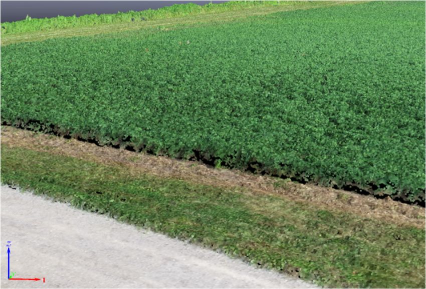
Remote Sens. 2021, 13, x FOR PEER REVIEW 3 of 16
Remote Sens. 2021, 13, 2487 3 of 15
2.5 cm resolution [11] and achieving this level of detail in the canopy model calls for lower
altitudes.
flight Alfalfa
altitudes. can becan
Alfalfa particularly challenging
be particularly since since
challenging once once
the canopy closes,
the canopy the field
closes, the
appears
field as a consistent
appears green
as a consistent surface
green that that
surface undulates
undulatesin windy conditions.
in windy This
conditions. type
This of
type
surface and the lower flight altitudes limit the unique and consistent
of surface and the lower flight altitudes limit the unique and consistent features features that the
photogrammetry model
photogrammetry model creation
creation process
process requires
requires in order to produce useful models. In
these challenging conditions, the process can
these challenging conditions, the process can simplysimply fail
fail or
or produce
produce unusable
unusable models
models with
with
many odd
many odd artifacts
artifacts and
and multiple
multiple ground
ground surfaces
surfaces (Figure
(Figure 1).
1).
Figure 1. Failed models from the photogrammetry process: (a) A model that generated only a few scattered points; (b) a
model that generated two intersecting ground planes; (c)
(c) aa side
side view
view of
of the
the intersecting
intersecting ground
ground planes
planes in
in (b).
(b).
The challenges
The challenges inin creating
creating alfalfa
alfalfa canopy
canopy models
models and
and the
the questions
questions fromfrom others
others mo-
mo-
tivated the goal of this study, which was to develop and compare alfalfa
tivated the goal of this study, which was to develop and compare alfalfa canopy models canopy models
derived from
derived from UAV
UAV imagery
imagery with
with different
different flight
flight parameters
parameters (altitude
(altitude and
and camera
camera angle).
angle).
Our initial
Our initialmotivation
motivationwas wastotoidentify
identifyanan efficient
efficient setset of flight
of flight parameters
parameters that that would
would reli-
reliably create successful models to enable the determination of canopy
ably create successful models to enable the determination of canopy heights within the 2.5 heights within
the resolution
cm 2.5 cm resolution
used in used
currentin current
manual manual field measurements
field measurements [11]. However,
[11]. However, other
other applica-
applications and uses of the 3D forage canopy models may call for different
tions and uses of the 3D forage canopy models may call for different accuracy levels. One accuracy
levels. One application
application of these
of these models is models is to use
to use them them to estimate
to estimate crop parameters
crop parameters such assuch as
yield.
yield. Therefore, to provide an illustration of the effects of these differences
Therefore, to provide an illustration of the effects of these differences in 3D canopy crea- in 3D canopy
creation,
tion, thesethese canopies
canopies werewere
used used
with with previously
previously developed
developed models models to estimate
to estimate yield
yield based
based
on 3D on 3D canopy
canopy point point
clouds.clouds.
In thisInstudy,
this study, our objective
our objective was was to conduct
to conduct an assessment
an assessment on
on the ability to successfully create 3D canopy models using various flight parameters.
the ability to successfully create 3D canopy models using various flight parameters. Ad-
Additionally, we wanted to ensure that the suggested methods work throughout the entire
ditionally, we wanted to ensure that the suggested methods work throughout the entire
alfalfa regrowth process—from the initial sparse plant crowns to the fully closed canopies
alfalfa regrowth process—from the initial sparse plant crowns to the fully closed canopies
before harvest. The results of this investigation will help engineers and researchers utilizing
before harvest. The results of this investigation will help engineers and researchers utiliz-
3D plant canopy models in the identification of the most useful and efficient methods to
ing 3D plant canopy models in the identification of the most useful and efficient methods
successfully create these models.
to successfully create these models.
2. Materials and Methods
2. Materials
2.1. Experiment andFields
Methods
2.1. Experiment Fields
In this study, we used two alfalfa fields, Field 1 and Field 2 (Figure 2), which are
In this
located at thestudy, we used
University two alfalfaNorth
of Kentucky’s fields,Farm
Fieldwith1 and
the Field 2 (Figure
approximate 2), which
centroid are
of each
located at the University of Kentucky’s North Farm with the approximate
field located at (38.128688, −84.509497) and (38.118587, −84.509612), respectively. The soil centroid of each
field
typeslocated
in Fieldat1 (38.128688,
were Armour −84.509497)
silt loam,andEgam (38.118587,
silt loam,−84.509612),
and Huntington respectively.
silt loam.The soil2
Field
types in Field
consisted 1 were silt
of Armour Armour
loam,silt loam, Egam
Huntington silt silt
loam,loam,
andand Huntington siltsilt
Bluegrass-Maury loam.
loam.Field
Data2
consisted
collection of Armour
occurred silt 17
from loam,
MayHuntington
2019 to 4 Junesilt 2019
loam,withandfour
Bluegrass-Maury silt loam. days.
separate data collection Data
The first alfalfa
collection cutting
occurred fromin the field for
17 May theto2019
2019 4 Junegrowing season
2019 with wasseparate
four cut on 7 data
May collection
2019 with
a JohnThe
days. Deere 630
first Discbine
alfalfa mower
cutting in the(Moline, Illinois)
field for the 2019and growing
collected season
as haylage
wason cut9 on
May7 2019.
May
This data collection period covered the alfalfa growth period between
2019 with a John Deere 630 Discbine mower (Moline, Illinois) and collected as haylage on the first and second
9cuttings of the
May 2019. Thisyear.
dataThe secondperiod
collection cuttingcovered
occurred theseveral
alfalfadays after
growth data collection
period between the ended.
first
Maturity
and second levels ranged
cuttings from
of the 0 toThe
year. 5 using
second thecutting
maturity stage evaluation
occurred several days scale
afterfrom
dataKalu
col-
and Fick
lection [33]. The
ended. alfalfa
Maturity in Field
levels 1 was
ranged a reduced
from lignin
0 to 5 using theand glyphosate
maturity stage resistant
evaluation variety,
scale
Ameristand
from Kalu and400 Fick
HVXRR,[33].and
Thethe alfalfa
alfalfa in in Field1 2was
Field wasaareduced
glyphosate resistant
lignin variety, Allied
and glyphosate re-
428RR. One herbicide spray application was performed during
sistant variety, Ameristand 400 HVXRR, and the alfalfa in Field 2 was a glyphosate the data collection period,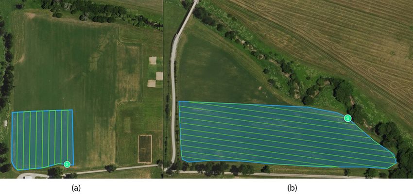
ually evaluated at 10 points (1 m sampling quadrats) in each field on each of the four
separate data collection days. After performing the drone flights on each day, the alfalfa
in each sampling quadrat was hand harvested, weighed, and dried to determine the dry
matter yield for each quadrat.
Remote Sens. 2021, 13, 2487 2.1.1. Field Conditions 4 of 15
Weed pressure was low throughout the sampling period in both fields, with nearly
all measured locations having less than 5% weed presence and only a minority in the 5%
to 20% range. Insect and disease pressure were initially similar to weed pressure, with
on 21 May 2019. Weed, insect, and disease pressure were manually evaluated at 10 points
most locations possessing less than 5% of plants exhibiting damage from insects or dis-
(1 m2 sampling quadrats) in each field on each of the four separate data collection days.
ease. However, insect and disease pressure increased during the data collection period
After performing
and by themore
4 June 2019, drone flights on
locations hadeach day, 5%
between the and
alfalfa
20%inofeach sampling
plants showingquadrat
damagewas
hand harvested, weighed,
from these sources. and dried to determine the dry matter yield for each quadrat.
Figure
Figure 2. Field
2. Field 1 (a)
1 (a) andand Field
Field 2 (b)
2 (b) outlined
outlined in blue.
in blue. TheThe green
green lines
lines show
show thethe
UAVUAV path
path when
when following
following a mission
a mission to to
cover
cover the entire field. The “S” indicates the starting point of
the entire field. The “S” indicates the starting point of the mission.the mission.
2.2. Data
Field Collection Process
Conditions
2.2.1. Ground Control Points
Weed pressure was low throughout the sampling period in both fields, with nearly
On eachlocations
all measured data collection
havingday, the first
less than 5% step
weedwas to record
presence andGround Control Points
only a minority in the 5%
(GCPs) and we also conducted our maturity, weed, insect, and disease
to 20% range. Insect and disease pressure were initially similar to weed pressure, evaluationswith
throughout
most locationsthe field. The less
possessing GCPs were
than 5%the brightly
of plants painted corners
exhibiting damageoffrom
sampling quadrats
insects or disease.
(10 per field
However, andand
insect 20 on each date),
disease which
pressure were distributed
increased during the in data
the field. These period
collection were rigid,
and by
located above the alfalfa canopy, and easily identifiable, which rendered
4 June 2019, more locations had between 5% and 20% of plants showing damage them good GCPs. from
The GCPs were located using a Trimble 5800 receiver (Trimble Inc., Sunnyvale, CA, USA)
these sources.
and the Lefebure NTRIP Client (Cedar Rapids, Iowa), which provided RTK corrections
from
2.2. theCollection
Data KentuckyProcess
Continuous Operated Reference Stations (KYCORS) network.
2.2.1. Ground Control Points
2.2.2. Flights
On each data collection day, the first step was to record Ground Control Points (GCPs)
After the GCPs were collected, three flight missions using different flight parameters
and we also conducted our maturity, weed, insect, and disease evaluations throughout the
were flown on each field using a DJI Phantom 4 Pro UAV (Shenzhen, China) for a total of
field. The GCPs were the brightly painted corners of sampling quadrats (10 per field and
six flights per day and 24 total unique flights. The Phantom 4 Pro has an integrated 20-
20megapixel
on each date), which
2.54 cm CMOSwere distributed
visible in the field.
camera mounted on These were
a gimbal. Therigid, located
camera above
lens has an the
alfalfa canopy, and easily identifiable, which rendered them good GCPs. The GCPs were
located using a Trimble 5800 receiver (Trimble Inc., Sunnyvale, CA, USA) and the Lefebure
NTRIP Client (Cedar Rapids, Iowa), which provided RTK corrections from the Kentucky
Continuous Operated Reference Stations (KYCORS) network.
2.2.2. Flights
After the GCPs were collected, three flight missions using different flight parameters
were flown on each field using a DJI Phantom 4 Pro UAV (Shenzhen, China) for a total
of six flights per day and 24 total unique flights. The Phantom 4 Pro has an integrated
20-megapixel 2.54 cm CMOS visible camera mounted on a gimbal. The camera lens has an
84◦ field of view and an 8.8 mm focal length. The missions were developed using DJI Go
and DJI GS Pro Mobile applications. All missions were set to have the images captured at
equal intervals perpendicular to the main path without stopping. The images had a front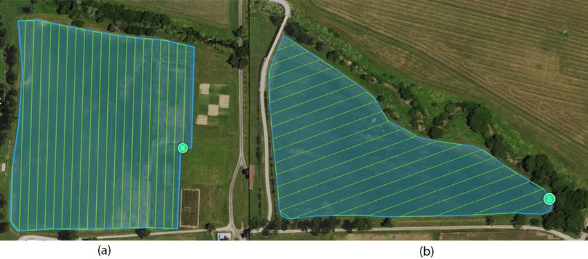
Remote Sens. 2021, 13, 2487                                                                                                                5 of 15

                              overlap of 85% and a side overlap of 75%. The flight parameters varied based on elevation
                              and gimbal angle (Table 1). Altering elevation and gimbal angle changed the resolution
                              and the mission planning app automatically adjusted flight speed to ensure image quality
                              (also shown in Table 1). In order to distinguish between these flight parameters (FP), they
                              will hereafter be referred to by the elevation and gimbal angle as the 50–90◦ , 50–75◦ , and
                              30–90◦ flight parameters.

                              Table 1. The flight parameters for the three types of missions.

                                                                   Flight Parameters 1        Flight Parameters 2       Flight Parameters 3
                                                                       (50–90◦ FP)                (50–75◦ FP)               (30–90◦ FP)
                                       Elevation (m)                       50.0                         50.0                   30.0
                                       Speed (m s−1 )                      5.70                         5.70                   3.30
                                      Gimbal Angle a                      −90.0◦                       −75.0◦                 −90.0◦
                                    Resolution (cm px−1 )                  1.40                         2.20                   0.80
                              a   Gimbal angle was measured from the horizontal.

                                   Missions providing complete field coverage took over 21 min for Field 1 (7.02 ha)
                              and over 10 min for Field 2 (3.09 ha), even when using the highest speed 50–90◦ flight
                              parameters (Table 2). However, the GCPs (based on equipment placement for another
                              experiment) were all located in a smaller region of each field. In order to reduce the flight
                              time, images captured, and the resulting processing time, the mission areas were reduced
                              from 7.02 ha to 1.3 ha for Field 1 and from 3.09 ha to 2.02 ha for Field 2 (Figure 3). Some of
                              the missions flown at 50 m still covered the entire field area to provide full field models,
                              but most flights were of the smaller partial field region. Whether or not a particular flight
                              (day/field/flight parameters) covered the entire field or part of the field is indicated in the
                              results. For this analysis, flight routes and mission durations are dependent on both flight
                              elevation and gimbal angle. The mission duration over the partial subsection of Field 1 at
                              50 m did increase by 45%, from 2 min 52 s to 4 min 9 s when the gimbal angle changed from
                              75◦ to 90◦ , even though the covered areas and flight elevation remained the same. Changes
                              to the flight route enabled by the difference in gimbal angle provided the time reduction.

                              Table 2. Mission characteristics when operating with each set of flight parameters in each field.

                                                                                    Field 1                              Field 2
                                                                            Full              Partial           Full               Partial
                                            Area (ha)                        7.02              1.30             3.09                2.02
                                   Mission Duration (min.:sec.)
                                            50–90◦ FP                       21:35               4:09            10:09               —a
                                            50–75◦ FP                        —a                 2:52            10:09               —a
                                            30–90◦ FP                        —a                10:36             —a                17:25
                                     Images Captured (count)
                                             50–90◦ FP                       513                 90             217                 —a
                                             50–75◦ FP                       —a                 61              217                 —a
                                             30–90◦ FP                       —a                 244             —a                  395
                              a   No mission was flown with these parameters on this field.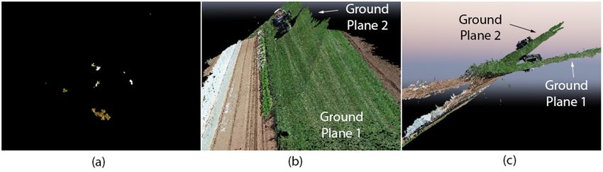
Remote Sens. 2021, 13, 2487 6 of 15
Remote Sens. 2021, 13, x FOR PEER REVIEW 6 of 16
Field 1 1(a)(a)partial ◦ flight parameters and Field 2 (b) partial field layout
Figure
Figure3. 3. Field partialfield
fieldlayout
layoutwith
withthe
the route
route for
for the
the 50–90
50–90° flight parameters and Field 2 (b) partial field layout
with thethe
route forfor
the 30–90 ◦
with route the 30–90°flight
flightparameters.
parameters.The
The “S”
“S” indicates the
the starting
startingpoint
pointofofthe
themission.
mission.
After
After flying
flying the
the three missions that
three missions thatprovided
providedscansscansofofthe
thefield,
field,a afourth
fourth mission
mission was
was
conducted
conducted thatthat flew
flew around each of
around each of the
the sampling
samplingquadrats
quadratsindividually.
individually.The TheUAVUAV was
was
flown
flownininaacircle
circle with
with a diameter of of between
between10 10m mand
and2020mmaround
aroundthe the quadrat
quadrat at at a height
a height
ofofapproximately
approximately 10 m. The The UAV
UAV flew
flew this
thiscircular
circularroute
routethree
threetimes
timesaround
around the
the quadrat
quadrat
with
withthe
the camera lockedonto
camera locked ontothethequadrat
quadrat while
while recording
recording videovideo (30 frames
(30 frames per second,
per second, 4K
4KUHD:UHD: 3840
3840 × 2160
× 2160 pixels).
pixels). This provided
This provided imageryimagery
of the of the alfalfa
alfalfa within within the quadrat
the quadrat from
from
manymany different
different anglesangles at a distance.
at a close close distance.
DuringDuring photogrammetry
photogrammetry processing, processing,
this videothis
video was subsampled
was subsampled and 30th
and every every 30thwas
frame frame was extracted.
extracted. This provided
This provided between 40 between
and 8040
and 80 images
images of each of each sampling
sampling quadrat.quadrat. For thisphotogrammetry
For this mission, mission, photogrammetry
processing processing
was per-
was performed
formed individually
individually for each for each using
quadrat quadrattheusing
images the images from
extracted extracted from the
the videos. videos.
Ground
control control
Ground points were
pointsnot used
were since
not usedeach
sincequadrat was isolated
each quadrat and its and
was isolated geometry kept it kept
its geometry at
itknown distance
at known fromfrom
distance the ground. All other
the ground. thingsthings
All other being being
equal, equal,
the photogrammetry
the photogrammetry pro-
cessing steps
processing were
steps the the
were same.
same.
2.2.3.
2.2.3.Photogrammetry Processing
Photogrammetry Processing
For
Foreach
each mission
mission and its set set of
ofimages,
images,we wecreated
createda anew new photogrammetry
photogrammetry project
project in in
Pix4Dmapper
Pix4Dmapper(Pix4D
(Pix4DS.A.,
S.A.,Prilly, Switzerland).
Prilly, Switzerland).Pix4D
Pix4D waswasselected as as
selected it was
it wasa photogrammetry
a photogram-
platform that has been
metry platform that used in many
has been usedof the previously
in many of thecited research projects
previously [13,14,25–27,29,31].
cited research projects
It[13,14,25–27,29,31]. It is based
is based on the computer visionontechniques
the computer visionand
of [34,35] techniques of [34,35]
implements variousand imple-
algorithms
ments various
described algorithms
in [36–38] described
to carry out theinphotogrammetry
[36–38] to carry out the photogrammetry
process. process.
The GNSS coordinates,
The GNSS system,
coordinate coordinates, coordinate
and camera system,
model wereand camera model
automatically were automatically
detected from the metadatade-
tected from
associated the each
with metadata
image associated with eachin
file. We operated image file. We
the World operated
Geodetic in the 1984
System World Geo- 96
(EGM
detic with
Geoid) System 1984 model
a camera (EGM code96of FC6310_8.8_5472x3648(RGB).
Geoid) with a camera The model code
images usedoffor
FC6310_8.8_5472x3648(RGB). The images used for a single model
a single model were loaded and the processing template “3D Model”, which set several were loaded and the
processing template “3D Model”, which set several program options,
program options, was chosen (Table 3). The images’ locations and layout were verified in was chosen (Table
3). The
map images’
view beforelocations andGCPs.
adding the layout were verified in map view before adding the GCPs.Remote Sens. 2021, 13, 2487 7 of 15
Table 3. Processing options set in Pix4Dmapper during 3D canopy model creation.
Processing Step Option
1. Initial Processing Keypoints Images Scale = Full
2. Point Cloud Mesh Export = LAS (a file format for saving point clouds)
Resolution = Automatic;
DSM (Digital Surface Model),
3. Use Noise Filtering (box is checked);
Orthomosaic, and Index.
Use Surface Smoothing (box is checked)—Type = Sharp.
Utilizing the GCP/MTP Manager, the GCPs for the given field were imported and
the Basic Editor tool was used to tag each GCP on 3–10 separate images. Once complete,
the rough locations of all the GCPs were verified in the map view and compared with
field notes to ensure the point had been marked correctly. Finally, we ran only the initial
processing step. The initial processing step could be completed rapidly while the final two
steps of model generation would take approximately one hour per 100 images. Verifying the
model after the initial processing enabled quick identification and resolution of any errors
detected at this stage. If failures were noted or the model did not pass the initial assessment
detailed in the next section, the initial processing step was repeated. After processing each
flight to create individual models, all the images from all three flights over a field on a
single day were processed together to create one final model (the Combined model).
2.2.4. Model Assessment
The Root Mean Square Error (RMSE) of the GCPs was a local indicator of how well
Pix4Dmapper fits the model to the GCPs. It represented the consistency between the geolo-
cation measured in the field and the geolocation Pix4Dmapper estimates when processing
the model. The goal was to minimize this value. In order to calculate RMSE, the error
between the actual location of each GCP and its location in the model was divided into
directional errors (X, Y, and Z components). All of the directional errors for all the GCPs
in a model were combined through the root-mean-square calculation to provide a RMSE
for each direction [39]. In order to provide a single value for a model, the three directional
RMSE values were averaged to create the Model RMSE. A Model RMSE of greater than
20 cm after the initial processing step indicated that this step had failed and that the project
should be recreated from the beginning. These failed models had generated a point cloud,
but it was corrupt and contained strange artifacts (e.g. Figure 1). Model RMSE varied for
the final 3D models but in all cases successful models had values much lower than 20 cm.
The ground sampling distance (GSD) was a measure of the spatial resolution of the
3D model and was defined as the distance between two neighboring pixels. A larger value
indicates a model with less detail. Higher flights at higher altitudes generally have higher
GSD values. The GSD is calculated separately for every pair of neighboring pixels in the
model. In order to provide a GSD value for the entire model, all of the individual GSDs in
the model were averaged together to produce the Model GSD. The final variable, which is
the camera optimization, is the percentage difference between the initial and optimized
parameters of the camera.
After processing each flight with GCPs and creating a final 3D canopy model, we
checked the model output. In the case of a completely failed model, Pix4DMapper would
provide an error stating that the process failed to produce any models. The model creation
process is a stochastic matching process and so it is affected by initial conditions. It can
potentially be trapped in the local minima of the optimization function. Simply repeating
the processing steps provided new initial conditions and often corrected issues within
this step. Once a model had completed processing without errors, the final Model RMSE,
Model GSD, and camera calibration difference were recorded.
2.2.5. Yield Estimation Using the 3D Canopy Models
For all the photogrammetry models, the 3D canopy inside the quadrats was isolated.
The point cloud from this canopy was processed following the procedure in [13] and theRemote Sens. 2021, 13, 2487 8 of 15
yield estimation models developed in [13] were applied to produce yield estimates in each
quadrat. In [13], yield models were developed using 2-variables, which were the mean and
standard deviation of the canopy heights, and 3-variables, which also added the average
maturity level of the field on that day to the mean and standard deviation of the canopy
heights that were used in the 2-variable model. Both of these models are Gaussian Random
Process models with rational quadratic kernel functions. The 2-variable and 3-variable
models were applied to each of the quadrat canopies. The estimates from these models
were then compared with the actual yield obtained by hand harvesting the quadrat. For
each set of flight parameters, the RMSE and R2 value for the relationship between the
estimated and actual yield was calculated.
3. Results
3.1. 3D Model Creation
The image sets from the 24 flights (two fields on four dates while using three dif-
ferent flight parameters) were processed individually and combined as described in the
methods section. This resulted in 32 unique models of the alfalfa canopy, which are sum-
marized in Table 4. Not all models completed the processing stage on the initial attempt.
Three models were processed twice and one model was processed three times before
successfully generating a 3D canopy as is noted in Table 4. In the end, Pix4D was able to
generate 3D canopy models for each one by following the procedures outlined above and
none of them possessed obvious errors such as multiple ground planes, strange artifacts,
or discontinuities.
Table 4. The properties of the 32 models that were processed in this study.
Flight Parameters Camera
Date Field Scan Model RMSE Calibration Model GSD
(dd/mm/yyyy) Field (Height (m)-Gimbal (Full/Partial) (cm) (cm)
Angle) Difference (%)
Field 1 30–90◦ Partial 0.50 4.44% 0.79
Field 1 50–75◦ Partial 1.00 2.55% 1.44
Field 1 c 50–90◦ Full 1.00 11.3% 1.38
17/05/2019 Field 1 Combined Combined 0.50 0.70% 1.35
Field 2 c 30–90◦ Partial 1.40 85.4% a 0.79
Field 2 50–75◦ Full 1.90 0.30% 1.41
Field 2 50–90◦ Full 2.10 0.45% 1.36
Field 2 Combined Combined 1.40 0.25% 1.23
Field 1 30–90◦ Partial 1.30 11.3% 0.79
Field 1 50–75◦ Partial 1.60 3.00% 1.39
Field 1 50–90◦ Partial 0.60 8.55% 1.28
21/05/2019 Field 1 Combined Combined 0.80 0.99% 0.81
Field 2 30–90◦ Partial 1.50 4.55% 0.77
Field 2 50–75◦ Full 1.70 1.09% 1.37
Field 2 50–90◦ Full 1.70 0.67% 1.34
Field 2 Combined Combined 1.30 0.13% 1.27
Field 1 30–90◦ Partial 2.50 14.1% 0.74
Field 1 50–75◦ Partial 2.00 4.62% 1.38
Field 1 50–90◦ Partial 2.40 5.49% 1.35
28/05/2019 Field 1 Combined Combined 2.20 0.07% 0.77
Field 2 c 30–90◦ Partial 13.1 b 14.3% 0.79
Field 2 d 50–75◦ Full 2.20 1.56% 1.46
Field 2 50–90◦ Full 5.70 0.56% 1.38
Field 2 Combined Combined 5.20 0.21% 1.31
Field 1 30–90◦ Partial 1.60 12.5% 0.76
Field 1 50–75◦ Partial 1.80 2.92% 1.42
Field 1 50–90◦ Partial 2.20 5.49% 1.36
04/06/2019 Field 1 Combined Combined 1.90 0.13% 0.79
Field 2 30–90◦ Partial 2.30 14.2% 0.75
Field 2 50–75◦ Full 2.20 1.08% 1.40
Field 2 50–90◦ Full 2.20 1.92% 1.33
Field 2 Combined Combined 2.00 0.10% 1.25
a Model had an unusually large camera calibration difference and was removed from further processing (entry italicized). b Model had an
unusually large Model RMSE and was removed from further processing (entry italicized). c Model was processed twice. These are the
results for the final processing run. d Model was processed three times. These are the results for the final processing run.Remote Sens. 2021, 13, 2487 9 of 15
Based on the extreme outliers in Model RMSE, camera calibration difference, and
Model GSD, two of the 32 models were judged not acceptable. One model had an unusually
large camera calibration difference of 85.4%, which was 38 times the median value of 2.24%
and the other had an unusually large Model RMSE of 13.1 cm, which was seven times
greater than the median value of 1.91 cm. These two models were considered failed
attempts. They were removed from further processing and not considered in any further
results. Note that these models were two of the four that had required additional processing
attempts to even create a 3D model in the first place. While the other two models that had
issues during initial processing did eventually result in acceptable models, the final outputs
of these two attempts were not acceptable. Thus, of the 32 models that were attempted, 30
of them produced acceptable models.
The values in Table 4 precisely describe the detail of the models, but images of the
models are also useful in understanding the model detail. Examples of a section of the
model created using the images captured with the 30–90◦ flight parameters on 4 June 2019
in Field 1 are shown in Figures 4–6. The images show that the models captured gaps in
Remote Sens. 2021, 13, x FOR PEER REVIEW
canopy coverage and details such as the wheeled traffic effects from a spray application10 of 16
Remote Sens. 2021, 13, x FOR PEER REVIEW 10 of 16
two weeks prior.
Figure 4.
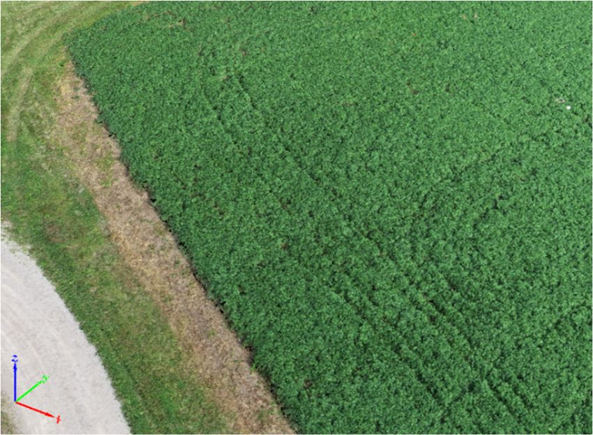
Figure 4. An
An isometric
isometric top
top view
view of
ofaaportion
portionofofaafully
fullyprocessed
processedalfalfa
alfalfamodel
modelofoffield
field1 1flown
flownonon 4
Figure 4. An isometric top view of a portion of apart
fully
of processed alfalfa ismodel of field 1 flown on 4
4June 2019
June 2019using
using
June recorded
2019 using
30–90°
30–90
30–90°
flight
◦ flight
flight
parameters.
parameters.Only
Only part thethe
of nearby barn
nearby barn modeled
is modeledas the
as flights
the flights
only one side of the parameters.
building. Only part of the nearby barn is modeled as the flights
only
only recorded
recorded one
one side
side of
of the
thebuilding.
building.
Figure 5. A side view of the alfalfa canopy in Field 1 from a portion of a fully processed model
Figureon
Figure
flown 5. A
5. 4AJune
side view
side viewusing
2019 ofthe
of the30–90°
alfalfacanopy
alfalfa canopy
flight ininField
Field11from
parameters. froma aportion
Althoughportion
theofofa afully
UAV fully processed
didprocessed
not model
model
take pictures flown
from
flown
on on
this4 angle 4 June 2019
and this
June 2019 using
close
using ◦30–90°
to the
30–90 flight
ground,
flight parameters. Although
the photogrammetry
parameters. Although theprocessthe UAV
UAV did did
captured not
not take take pictures
thepictures
transition from
from
from this
this angle
the short and this close to the ground, the photogrammetry process captured the transition from
angle andgrass bordering
this close to thethe field tothe
ground, thephotogrammetry
taller alfalfa plants.
process captured the transition from the
the short grass bordering the field to the taller alfalfa plants.
short grass bordering the field to the taller alfalfa plants.Figure 5. A side view of the alfalfa canopy in Field 1 from a portion of a fully processed model
Remote Sens. 2021, 13, 2487 flown on 4 June 2019 using 30–90° flight parameters. Although the UAV did not take pictures 10 from
of 15
this angle and this close to the ground, the photogrammetry process captured the transition from
the short grass bordering the field to the taller alfalfa plants.
Figure 6.
Figure 6. An
An aerial
aerial view
view of
of the
the alfalfa
alfalfa canopy
canopy in
in field
field 11 and
and tracks
tracks from
fromwheeled
wheeledtraffic
trafficon
onaaportion
por-
tion of a fully processed model flown on 4 June 2019 using 30–90°
◦ flight
of a fully processed model flown on 4 June 2019 using 30–90 flight parameters. parameters.
The results from the individual models were compiled by flight parameters used in
the flight to capture the model data (Table 5). The largest effect of the flight parameters
was on the GSD. The flights at an altitude of 30 m had a much lower mean Model GSD
compared to the flights at 50 m, as would be expected with models based on images taken
at different altitudes. This corresponds to finer detail in the models from the flights at 30 m.
There was also little variation (low standard deviation) in the GSD between models created
using a given flight parameter. For all models created using the 30–90◦ flight parameters,
the GSD was always less than 1 cm. For models created using 50–75◦ and 50–90◦ flight
parameters, the GSD was always below 1.5 cm.
Table 5. Model GSD by flight parameters used in flights (including both fields on all four sampling days).
Flight Parameters Model GSD (cm)
(Height (m)-Gimbal Angle) Min. Max. Mean Std. Dev
30–90◦ 0.740 0.790 0.767 0.021
50–75◦ 1.37 1.46 1.41 0.030
50–90◦ 1.28 1.38 1.35 0.032
Combined 0.770 1.35 1.09 0.257
There were fewer significant differences in the Model RMSE values (Table 6). While
the models created using the images from the flights at 30 m did have lower mean Model
RMSE, there were no significant differences (using α = 0.05) between the Model RMSE
values based on flight parameters. Maximum RMSE values (from acceptable models) were
as high as 5.7 cm, but such high values were rare. Of the 30 acceptable models, 28 models
had Model RMSE values less than 2.5 cm.
Table 6. Model RMS Error by flight parameter used in flights (including both fields on all four
sampling days).
Flight Parameters Model RMS Error (cm)
(Height (m)-Gimbal Angle) Min. Max. Mean Std. Dev
30–90◦ 0.500 2.50 1.62 0.722
50–75◦ 1.00 2.20 1.80 0.389
50–90◦ 0.600 5.70 2.24 1.54
Combined 0.500 5.20 1.91 1.45
Interestingly, the combination models performed worse than models based on images
taken only at 30 m. The additional images from the two flights using the 50 m flightRemote Sens. 2021, 13, 2487 11 of 15
parameters did not improve the model creation process. They only appeared to increase
additional processing time.
3.2. Yield Estimation
There were 10 sampling quadrats per field on each of the four sampling days. This
corresponds to a total of 80 samples for each flight parameter. However, not all samples
created 3D canopy point clouds that could be used in the yield estimation model. The most
common issue was that the highly visible geometric structure of the sampling quadrat
would create canopy distortions inside the sampling region and the point cloud processing
steps used to estimate yield would fail. Of the 80 possible quadrat samples, there were
75, 34, 34, 28, and 72 usable samples for the yield estimation model from the Quadrat
Only, 30–90◦ , 50–90◦ , 50–75◦ , and the Combination model, respectively. The Quadrat Only
and Combination models had more views of the quadrats from different angles, which
appeared to assist those models by reducing distortions from the quadrats. In actual field
usage, the sampling quadrats should not be an issue since they are not normally present
during alfalfa production. Future work with complete field imagery at 30 m and 50 m
elevations will need to use different sampling quadrats to eliminate the introduction of
artificial structures to the field canopy.
When the 3D canopy models were combined with the yield estimation models pre-
sented in [13], the yield estimation accuracy mostly aligned (Table 7) with the previously
discussed canopy model accuracy represented by the Model RMS Error. The 50–75◦ and
the 30–90◦ FP did better than the 50–90◦ and the combined models. However, for yield
estimation, the 50–75◦ FP had the lowest error and the highest R2 values when used to
predict the yield within the test quadrats. The next best set of flight parameters that cov-
ered the entire field was the 30–90◦ FP. The combined FP created the worst yield estimates.
This set of data also included the Quadrat Only FP which consisted of individual canopy
models created for each yield sampling quadrat at a height of approximately 10 meters
with varying non-nadir gimbal angles. Although the Quadrat Only FP had the lowest
flight altitude and had independent 3D canopies for each quadrat, it was only about as
accurate as the 30–90◦ FP. The error rates and R2 values are different when the canopies
are used in the 2-variable and 3-variable models, but the trends remain similar with both
approaches for estimating yield: 50–75◦ FP produced the best estimates and the Combined
FP produced the worst.
Table 7. Yield estimation accuracy using the 3D canopy models from different flight parameters.
3-Variable 2-Variable Average
Flight Parameters Model Model (Both Models)
(Height (m)-Gimbal
Angle) RMSE RMSE RMSE
R2 R2 R2
(kg ha−1 ) a (kg ha−1 ) a (kg ha−1 ) a
Quadrat Only 907 0.71 821 0.60 864 0.65
30–90◦ 780 0.68 897 0.30 838 0.49
50–75◦ 490 0.87 354 0.84 422 0.85
50–90◦ 1045 0.55 966 0.35 1005 0.45
Combined 1298 0.53 1353 0.47 1325 0.50
Average 904 0.67 878 0.51 891 0.59
a Maximum yield was 3800 kg ha−1 .
The 2-variable and 3-variable models were created using individual flights and 3D
models for each sampling quadrat in a manner that is most similar to the Quadrat Only
FP presented in Table 7. In [13], the 2-variable and the 3-varible model were found to
predict yields with RSME/R2 of 799 kg ha−1 /0.63 and 734 kg ha−1 /0.69, respectively.
These are similar to the values obtained with the Quadrat Only FP parameters. This set of
experiments was conducted in different fields in a different growing year and so both yield
estimation models are consistent even with the changes in varieties, fields, and weatherRemote Sens. 2021, 13, 2487 12 of 15
conditions. As in [13], the 3-variable model performed better than the 2-variable model
with lower RMS Error and higher R2 values when considering the average of all flight
methods. However, for the 30–90◦ and 50–90◦ flight parameters with the 2-variable model,
the R2 values fell below 0.4 and so the 2-variable model does not work well with those
flight parameters. Interestingly, using the 50–75◦ FP produced better results than the
high-resolution models from the Quadrat Only canopies. The RMSE and R2 values for
yield estimates with the 50–75◦ FP were even better than those obtained when initially
creating the models.
4. Discussion
While 94% of the 32 attempted models were created successfully, the two failed models
demonstrate that these flight parameters are not foolproof. If a model is being used for
mission critical decision making and a usable model is crucial, multiple flights using
different flight parameters may be warranted. In cases where a model failed in this study,
the models based on a different set of flight parameters over the same field at the same time
were always able to create a successful model. The canopies captured during this project
include entire whole alfalfa forage growth cycle. They start at seven days after cutting
when regrowth was just beginning. The final canopy was measured 28 days after cutting
when the crop was, again, ready for harvest. Therefore, these parameters appear acceptable
for utilization in modeling the canopy during the entire growth cycle of the alfalfa forage.
The models produced with the 30–90◦ FP were more detailed as determined by the
GSD, but they were not more accurate based on the lack of significant differences in Model
RMSE between the different flight parameters. These models were also less accurate when
used to predict yield. We also found little benefit from combining images from flights
with multiple parameters. While the combined models did appear to have a denser point
cloud than many of the other models, the additional processing time, minimal difference in
model accuracy parameters, and the lower ability to predict alfalfa yield when used with
the alfalfa yield prediction models suggests that this approach is actually detrimental to
the usefulness of a model.
We suggest using the 50–75◦ parameters for the creation of alfalfa canopies with the
3-variable model for predicting yield. Lower altitudes required much longer flight and
processing times and the models were not always acceptable after processing. In comparing
the gimbal angles at 50 m, the 75◦ gimbal angle provided more consistent Model RMSEs
that were always less than 2.2 cm, unlike the 90◦ gimbal angle which had a maximum of
5.7 cm. The tests, when using the different flight parameters to predict alfalfa yield, further
strengthen this suggestion. The 50–75◦ parameters were clearly the best for this particular
use. The 3-variable model was more consistent across flight parameters, which could be
useful for real world applications where field elevation changes may make it difficult to
maintain an exact flight height above the ground. While the 2-variable model with the
50–75◦ parameters had slightly lower RMSE than the 3-variable model, its R2 with all flight
parameters was always lower than the 3-variable model. In certain situations, the R2 could
be as low as 0.30 (30–90◦ ) or 0.35 (50–90◦ ). In our previous study, the RMSE followed the
trend of the R2 values with the 3-variable model providing better results than the 2-variable
model. For the sake of consistency, the 3-variable model appears to be the better option.
Further testing would be necessary to see if flights at slightly higher altitudes may also
provide acceptable accuracy levels, but based on the results of other studies we should see
deteriorating accuracies and detail as we increase in height [27,28,30,31].
Comparisons with Other Studies
While other studies aimed at estimating biomass or crop yield did not report the
effect of varying flight heights, they flew missions at similar heights between 30 m and
50 m above ground level. However, these studies all appeared to use cameras with a 90◦
gimbal angle. The results of our study indicate that switching to a 70◦ gimbal angle has the
potential to improve crop height models and, thus, their biomass or yield estimation results.Remote Sens. 2021, 13, 2487 13 of 15
A major difference between our study and the other photogrammetry studies is our
focus on the ability to reliably create an acceptable model and consistently estimate alfalfa
yield correctly. Our study performed multiple repetitions of flights using each flight
parameter on different days and on multiple fields. In commercial alfalfa production,
farmers must periodically assess the crop to determine appropriate harvest time as well as
other production decisions such as when to spray various chemicals. The crop is constantly
developing and timely information is critical in the production decision making process.
In this project, we followed this periodic monitoring requirement and flew every seven
days exactly. Other studies had different goals and many based their analysis on a single
set of flights. Since they were not flying on a set schedule, they could have waited for
perfect flight capture conditions (e.g. no wind) and repeated any flights that provided
unacceptable results after photogrammetry processing. It is also possible that the fields
and environments targeted in these studies have enough natural variation that model
failure is not an issue. Given the inquiries into our methods and our own difficulty in
initially identifying appropriate flight parameters, consistency and reliability are important
additional factors, which this study has addressed.
5. Conclusions
Based on this study, we suggest the utilization of a set of flight parameters for creating
3D models of alfalfa canopies. Following the procedures provided here, producers and
researchers can be confident that they will consistently be able to generate a 3D canopy
model with a single coverage flight based on our acceptable model creation rate of 94%.
Furthermore, this remains true for all of the alfalfa growth stages from initial regrowth from
sparse crowns to a fully closed canopy. In the cases where one of our canopy models was
not acceptable, our other trials on that day and in that field did provide acceptable models.
If a successful 3D canopy model is absolutely required, it is suggested that a second flight
with different image capture points be performed. Model detail (measured by GSD) varied
by flight altitude and gimbal angle between the means of 0.767 cm for the 30–90◦ flight
parameters and 1.41 cm with the 50–75◦ flight parameters. However, the geolocation error
(measured by Model RMSE) was similar for the different flight parameters with an overall
mean of 1.91 cm. When these canopies were used with alfalfa prediction models, the 50–75◦
flight parameter clearly provided the best estimate of alfalfa yield. Given the lower flight
durations and processing times as well as increased consistency in geolocation accuracy,
most users should opt for flights with a 50 m altitude and 75◦ gimbal angle. If the target
application for the 3D canopy is alfalfa yield estimation, then the 50–75◦ flight parameter is
strongly suggested.
Author Contributions: Conceptualization, J.D. and J.J.; methodology, C.M., J.D., J.J., and S.T.S.;
formal analysis, S.T.S. and C.M.; investigation, C.M. and J.D.; resources, J.D.; data curation, C.M. and
S.T.S.; writing—original draft preparation, C.M.; writing—review and editing, J.D., S.T.S., and J.J.;
visualization, C.M. and S.T.S.; supervision, J.D.; project administration, J.D.; funding acquisition, J.D.
and J.J. All authors have read and agreed to the published version of the manuscript.
Funding: This work is supported by the Alfalfa and Forage Research Program grant no. 2016-70005-
25648 /project accession no. 1010223 from the USDA National Institute of Food and Agriculture.
Data Availability Statement: Upon acceptance of this manuscript, we will work with the editor
to determine the appropriate public posting location for the data from this project. The raw im-
ages are approximately 50 GB and the photogrammetry models are also very large, which limits
posting locations.
Conflicts of Interest: The authors declare no conflict of interest. The funders had no role in the design
of the study; in the collection, analyses, or interpretation of data; in the writing of the manuscript or
in the decision to publish the results.Remote Sens. 2021, 13, 2487 14 of 15
References
1. Nelson, B. Alfalfa Remains Country’s 3rd Most Valuable Field Crop; National Alfalfa & Forage Alliance: St. Paul, MN, USA, 2019.
2. NASS. Crop Values 2017 Summary; United State Department of Agriculture, National Agricultural Statistics Service: Washington,
DC, USA, 2018.
3. Lamb, J.F.S.; Sheaffer, C.C.; Samac, D.A. Population Density and Harvest Maturity Effects on Leaf and Stem Yield in Alfalfa.
Agron. J. 2003, 95, 635–641. [CrossRef]
4. Ball, D.M.; Collins, M.; Lacefield, G.D.; Martin, N.P.; Mertens, D.A.; Olson, K.E.; Putnam, D.H.; Undersander, D.J.; Wolf, M.W.
Understanding Forage Quality; American Farm Bureau Federation Publication: Park Ridge, IL, USA, 2001; Volume 1.
5. Saha, U.K.; Sonon, L.S.; Hancock, D.W.; Hill, N.S.; Stewart, L.; Heusner, G.L.; Kissel, D.E. Common Terms Used in Animal Feeding
and Nutrition; University of Georgia, College of Agricultural and Environmental Sciences: Athens, GA, USA, 2017.
6. Undersander, D.; Hall, M.H.; Vassalotti, P.; Cosgrove, D. Alfalfa Germination & Growth; University of Wisconsin-Extension
Cooperative Extension: Madison, WI, USA, 2011; p. 18.
7. Ball, D.M.; Hoveland, C.S.; Lacefield, G.D. Southern Forages; Potash & Phosphate Institute, Foundation for Agronomic Research:
Atlanta, GR, USA, 1991; ISBN 978-0-9629598-1-3.
8. Hancock, D.W.; Buntin, G.D.; Ely, L.O.; Lacy, R.C.; Heusner, G.L.; Stewart, R.L. Alfalfa Management in Georgia; University of
Georgia, College of Agricultural and Environmental Sciences: Athens, GA, USA, 2009.
9. Undersander, D.; Cosgrove, D.; Cullen, E.; Grau, C.; Rice, M.E.; Renz, M.; Sheaffer, C.C.; Shewmaker, G.; Sulc, M. Alfalfa
Management Guide; American Society of Agronomy: Madison, WI, USA, 2011; ISBN 0-89118-179-2.
10. Hintz, R.W.; Albrecht, K.A. Prediction of Alfalfa Chemical Composition from Maturity and Plant Morphology. Crop Sci. 1991, 31.
[CrossRef]
11. Lang, B. Estimate First Crop Pre-Harvest Alfalfa Quality in the Field Using PEAQ; Iowa State University Extension and Outreach
Publication: Ames, IA, USA, 2017; pp. 1–2.
12. Mueller, S.C.; Teuber, L.R. Alfalfa Growth and Development. In Irrigated Alfalfa Management for Mediterranean and Desert Zones;
Summers, C.G., Putnam, D.H., Eds.; University of California Alfalfa & Forage Systems Workgroup: Davis, CA, USA, 2007.
13. Dvorak, J.S.; Pampolini, L.F.; Jackson, J.J.; Seyyedhasani, H.; Sama, M.P.; Goff, B. Predicting Quality and Yield of Growing Alfalfa
from a UAV. Trans. ASABE 2021, 64, 1. [CrossRef]
14. Brodbeck, C.; Sikora, E.; Delaney, D.; Pate, G.; Johnson, J. Using Unmanned Aircraft Systems for Early Detection of Soybean Diseases;
Cambridge University Press: Edinburgh, UK, July 2017; Volume 8, pp. 802–806.
15. Vanegas, F.; Bratanov, D.; Powell, K.; Weiss, J.; Gonzalez, F. A Novel Methodology for Improving Plant Pest Surveillance in
Vineyards and Crops Using UAV-Based Hyperspectral and Spatial Data. Sensors 2018, 18, 260. [CrossRef]
16. Chang, A.; Jung, J.; Maeda, M.M.; Landivar, J. Crop Height Monitoring with Digital Imagery from Unmanned Aerial System
(UAS). Comput. Electron. Agric. 2017, 141, 232–237. [CrossRef]
17. Enciso, J.; Avila, C.A.; Jung, J.; Elsayed-Farag, S.; Chang, A.; Yeom, J.; Landivar, J.; Maeda, M.; Chavez, J.C. Validation of
Agronomic UAV and Field Measurements for Tomato Varieties. Comput. Electron. Agric. 2019, 158, 278–283. [CrossRef]
18. Madec, S.; Baret, F.; de Solan, B.; Thomas, S.; Dutartre, D.; Jezequel, S.; Hemmerlé, M.; Colombeau, G.; Comar, A. High-
Throughput Phenotyping of Plant Height: Comparing Unmanned Aerial Vehicles and Ground LiDAR Estimates. Front. Plant Sci.
2017, 8, 2002. [CrossRef] [PubMed]
19. Watanabe, K.; Guo, W.; Arai, K.; Takanashi, H.; Kajiya-Kanegae, H.; Kobayashi, M.; Yano, K.; Tokunaga, T.; Fujiwara, T.; Tsutsumi,
N.; et al. High-Throughput Phenotyping of Sorghum Plant Height Using an Unmanned Aerial Vehicle and Its Application to
Genomic Prediction Modeling. Front. Plant Sci. 2017, 8, 421. [CrossRef]
20. Feng, A.; Zhang, M.; Sudduth, K.A.; Vories, E.D.; Zhou, J. Cotton Yield Estimation from UAV-Based Plant Height. Trans. ASABE
2019, 62, 393–404. [CrossRef]
21. Huang, Y.; Brand, H.J.; Sui, R.; Thomson, S.J.; Furukawa, T.; Ebelhar, M.W. Cotton Yield Estimation Using Very High-Resolution
Digital Images Acquired with a Low-Cost Small Unmanned Aerial Vehicle. Trans. ASABE 2016, 59, 1563–1574. [CrossRef]
22. Bendig, J.; Bolten, A.; Bennertz, S.; Broscheit, J.; Eichfuss, S.; Bareth, G. Estimating Biomass of Barley Using Crop Surface Models
(CSMs) Derived from UAV-Based RGB Imaging. Remote Sens. 2014, 6, 10395–10412. [CrossRef]
23. Lu, N.; Zhou, J.; Han, Z.; Li, D.; Cao, Q.; Yao, X.; Tian, Y.; Zhu, Y.; Cao, W.; Cheng, T. Improved Estimation of Aboveground
Biomass in Wheat from RGB Imagery and Point Cloud Data Acquired with a Low-Cost Unmanned Aerial Vehicle System. Plant
Methods 2019, 15, 17. [CrossRef]
24. Yue, J.; Yang, G.; Li, C.; Li, Z.; Wang, Y.; Feng, H.; Xu, B. Estimation of Winter Wheat Above-Ground Biomass Using Unmanned
Aerial Vehicle-Based Snapshot Hyperspectral Sensor and Crop Height Improved Models. Remote Sens. 2017, 9, 708. [CrossRef]
25. Shi, Y.; Thomasson, J.A.; Murray, S.C.; Pugh, N.A.; Rooney, W.L.; Shafian, S.; Rajan, N.; Rouze, G.; Morgan, C.L.S.; Neely, H.L.;
et al. Unmanned Aerial Vehicles for High-Throughput Phenotyping and Agronomic Research. PLoS ONE 2016, 11, e0159781.
[CrossRef] [PubMed]
26. Gauci, A.A.; Brodbeck, C.J.; Poncet, A.M.; Knappenberger, T. Assessing the Geospatial Accuracy of Aerial Imagery Collected with
Various UAS Platforms. Trans. ASABE 2018, 61, 1823–1829. [CrossRef]
27. Mesas-Carrascosa, F.-J.; Torres-Sánchez, J.; Clavero-Rumbao, I.; García-Ferrer, A.; Peña, J.-M.; Borra-Serrano, I.; López-Granados,
F. Assessing Optimal Flight Parameters for Generating Accurate Multispectral Orthomosaicks by UAV to Support Site-Specific
Crop Management. Remote Sens. 2015, 7, 12793–12814. [CrossRef]You can also read